NOMENCLATURE
- A
-
model constant defined in Lefebvre's model for LBO
- AFR
-
air to fuel ratio
- D p
-
initial mean drop size, micron
- D p,crit
-
critical droplet diameter
- D r
-
mean drop size relative to JP4
- d t
-
throat diameter of venturi, mm
- DPM
-
discrete phase model
- FV-LBO
-
flame volume-based lean blow-out model
- K
-
model constant defined in FV model
- LBO
-
lean blow-out
- LHVr
-
lower calorific value relative to JP4
- LDI
-
lean direct injection
- LPP
-
lean pre-mixed and pre-vaporised
- f PZ
-
fraction of air entering the primary zone
-
 $\bar{f}$
-
Favre mean mixture fraction
-
$\overline {{f^{'2}}} $
-
variance of mixture fraction
- ma
-
total mass flow rate of combustor inlet, kg/s
- mf
-
mass flow rate of fuel, kg/s
- mpri
-
mass flow rate through primary swirler, kg/s
- msec
-
mass flow rate through secondary swirler, kg/s
- P3
-
inlet pressure, Kpa
-
probability density function
- qLBO
-
overall fuel/air ratio at lean blow-out, g/kg
- qLBO, predict
-
lean blow-out predicted by empirical model, g/kg
- r
-
correlation coefficient
- IRZ
-
inner recirculation zone
- T 3
-
inlet temperature of combustor, K
- T crit
-
threshold value of temperature, K
- V c
-
combustor volume ahead of dilution holes, m3
- Vf
-
flame volume, m3
- Vf ,n
-
flame volume obtained by fuel concentration contour, m3
- α
-
fraction of dome air
- β
-
dimensionless flame volume defined as Vf /Vc
- βf,n,c
-
dimensionless flame volume defined as V f,n,c/Vc
- ρ
-
density, kg/m3
- μ l
-
laminar viscosity, kg/(s·m)
- μ t
-
turbulent viscosity, kg/(s·m)
- δ
-
angle of flare outlet, °
- λr
-
effective evaporation coefficient relative to JP4
- Δx
-
thickness, mm
- Z i
-
elemental mass fraction of element, i


1.0 INTRODUCTION
Blow-out refers to situations where the flame becomes detached from the location where it is anchored and is physically ‘‘blown out’’ of the combustor(Reference Lieuwen, McDonell, Santavicca and Sattelmayer1). It is essentially flame extinction at flowing conditions. In gas turbine combustion, Lean Blow-Out (LBO) limit is a term referring to the equivalence ratio at which flame blow-out occurs when operated at lean fuel conditions(Reference Li, Zhang, Zhong, Weng, Li and Zhu2). The flame can only be stabilised above the LBO limit. It defines a very important boundary to keep off in land-based gas turbine operation; LBO event usually requires a lengthy and costly gas turbine shutdown, purge and restart. In aero engines, LBO events may invoke safely concerns for the vehicle and, therefore must be avoided. Hence, LBO is a fundamental performance and safety parameter in an air-breathing engine and the operating envelope of the engine is bounded by the lean limit. Over the last two decades, the technology focus has shifted towards the development of lean combustors to meet emission standards. This has confronted designers with a challenge to develop combustors, which must operate near lean limits without compromising safety and operational requirements. Moreover, it has elevated the significance of LBO prediction, than ever. Hence, a simple and straightforward tool is desirable by the industry for the LBO prediction with satisfactory accuracy. Given the importance of fuel-lean flames for practical combustion applications, a significant amount of literature can be found on LBO prediction. However, based on the conceptual approaches, one may classify them into the following three categories: semi-empirical methods, numerical simulations and hybrid methods. Hybrid methods are comparatively recent, and they make use of both semi-empirical and numerical simulations.
The pioneer work on semi-empirical methods can be traced back to Perfect Stirred Reactor (PSR) models(Reference Longwell and Weiss3,Reference Longwell, Frost and Malcolm4) and Characteristic Time (CT) models(Reference Zukoski and Marchble5). Both CT and PSR models are outcomes of flame stabilisation analysis conducted on a bluff body, especially the one seen in afterburners. In PSR models, LBO occurs when the heat release rate is less than heat loss rate. In CT models, LBO occurs when the fuel residence time in the shear layer is less than the sum of evaporating time and chemical reaction time. Based on the criterion for LBO judgments, PSR and CT models are established based on energy and time scales balances, respectively. These models serve as the basis for the existing theoretical models for LBO in gas turbine engines. Mellor(Reference Mellor, Jarymowycz, Stow and Dowling6-Reference Leonard, Mellor, Ley and Yates9) suggested improvements to CT model by defining three characteristics times: shear layer mixing time, fuel vapour ignition delay time and droplet evaporation time. The main improvement in the PSR model and its precise application in gas turbine combustors is presented by Lefebvre(Reference Ballal and Lefebvre10-Reference Lefebvre12). He successfully included terms for entrainment, heterogeneity of fuel/air mixture, fuel atomisation, operating conditions and geometry of combustor in the empirical correlation. For these reasons, his model is considered to be the most general model for LBO predictions. Many research studies have focused on LBO performance of combustors with swirl cups. The excellent behaviour of swirl cups in terms of flame stability, efficiency, exit temperature profile, emissions, etc. has made them universal in modern aero engines. The best examples are CFM-56 and CFM-80(Reference Mellor8). Ateshkadi et al(Reference Ateshkadi, McDonell and Samuelsen13) presented the effect of mixer components on LBO and established an improved correlation based on Lefebvre's model. But, owing to insufficient modelling depth of these semi-empirical correlations, a prediction accuracy of only approximately ±35% has been reported so far.
Over the last decade, there has been exponential improvement in computational power and development of numerical codes. Numerical methods, especially Large Eddy Simulations (LES), have made it possible to model combustion transients’ phenomena with high temporal and spatial resolution. During the past decade, LES has developed in a variety of directions: a linear eddy model (LEM)(Reference Menon14-Reference Eggenspieler and Menon17), an Eddy Break-up Model (EBM)(Reference Kim, Lienau, Van Slooten, Colket, Malecki and Syed18), an eddy dissipation concept (EDC)(Reference Gokulakrishnan, Bikkani, Klassen, Roby and Kiel19), and probability density functions (PDF)(Reference Gokulakrishnan, Foli, Klassen, Roby, Soteriou, Kiel and Sekar20). Menon, based on LES-LEM(Reference Menon, Stone and Patel16,Reference Eggenspieler and Menon17,Reference Porumbel and Menon21) , attained the flame distortion and variation in flame spread velocity but did not succeed in capturing eddies that mostly effect the local extinction. Kim and Lienau(Reference Kim, Lienau, Van Slooten, Colket, Malecki and Syed18) studied LBO in gas turbine flame holder applications using LES and eddy breakup (EBU). Among the selected seven operating conditions (ϕ = 0.2, 0.5, 0.52, 0.6, 0.7, 1.0, 1.62), predictions in only two conditions were consistent with respective experimental data. Some LES studies have also been done on the stability of flame on V-gutters by Smith(Reference Smith, Nickolaus, Leach, Kiel and Garwick22,Reference Khosla, Leach and Smith23) . Large-eddy simulation coupled with a Filtered Density Function (FDF) and Conditional Moment Closure (CMC) are the most promising methods to date. FDF is able to capture the interaction between hydrodynamics and chemical kinetics, making it possible to predict the occurrence of slow chemistry effects, extinction and possibly re-ignition. FDF methods have also been applied to the modelling of particulates (soot) formation in turbulent non-premixed combustion, but a computational research study(Reference Ge, Cleary and Klimenko24) on Sandia flame E demonstrates that 5-10 days is the possible solution time for simple laboratory scales flames. On the other hand, the CMC model has proven to accurately capture blow-off velocity(Reference Tyliszczak, Cavaliere and Mastorakos25), providing a notable example of successful numeric prediction of LBO. It offers a way to capture the localised extinction and the global blow-off in swirl-stabilised flames, but also requires calibration of constants for the scalar dissipation rate based on the pilot scale burner. This puts a limit on the universal utilisation of this technique and needs further evaluation for capturing quantitatively realistic flame extinction. Moreover, simulations of 1 ms of the physical time required approximately three hours on a PC cluster with 4×8 processors with reported iterative time steps equal to Δt = 5.0 × 10⁻⁶ s. Hence, a 1 s simulation would require 96,000 CPU hours. The CFD and CMC meshes consisted of 3 × 10⁶ and 54,000 hexahedral cells, respectively. Another LBO study by Smith(Reference Black and Smith26) suggests that a typical LES requires 20 days using 16.9 GHz PCs. An additional built-in limitation is chemistry stiffness, a problem emphasised by Pope(Reference Pope27). Hence, LBO predictions involving LES-based simulation are not only expensive but are also lacking in their universal application due to the calibration of constants based on laboratory-scale flames.
The prediction of LBO with empirical correlation is economical, but it has a two shortcomings: prediction accuracy and low universality for different combustor configurations. Likewise, LES with the CMC model is the best predicting solution for simulating transients in a gas turbine combustor, but these simulations are very expensive and demand calibrations of constants. Based on these demonstrated deficiencies of semi-empirical and numerical methods, a hybrid approach has evolved as a promising prediction tool for practical combustors. The hybrid methodology, uniting the advantages of empirical correlations and computational development, pledges robust and accurate LBO predictions. The inadequacies in empirical correlations can be compensated with CFD. For the first time, Sturgess et al(Reference Sturgess and Shouse28) presented hybrid modelling approach for LBO predictions based on serial application of CFD and detailed kinetics network solution, respectively. At the representative operating conditions of interest, the CFD solution is obtained. The field solutions resulting from the CFD calculation is post-processed using a dissipation gradient analysis and topology methods to represent the fluid dynamics by means of a connected network of fuel/air mixers, PSRs and plug-flow reactors. Detailed chemistry is solved on the network over the required range of operating conditions near LBO to yield the desired solutions. In a different study(Reference Sturgess, Gogineni and Shouse29), Sturgess concluded that relatively minor geometric changes in a combustor liner with a fixed-geometry swirl generator module can result in very significant shifts in the primary zone. Global LBO stability, owing to complex local flame holding behaviour, is strongly associated with the detailed interactions of the swirling and transverse jet systems.
The current work focuses on the improvement of hybrid models presented previously by the authors. Flame Volume Lean Blow-Out (FV-LBO) is a combination of a semi-empirical correlation and a numerical scheme termed Fuel Iterative Approximation (FIA). FV-LBO model is the improved version of Lefebvre's LBO model while FIA is an iterative computational method based on Reynolds-averaged Navier-Stokes equations (RANS). The core issue in hybrid methodology is associated with the estimation of flame volume (V f ). It is strongly associated by swirl cup assembly and liner configuration, turbulence intensity, heat liberation, volumetric expansion and the flapping frequency of the flame. Hence, V f can be considered as a one lumped parameter representing the complex interdependence of many geometric and thermodynamic parameters, and its realistic estimation is a challenge. Previously; flame volume was predicted from concentration contours based on cold flow simulations; the estimation value is underpredicted and requires correction before utilising it in LBO correlations. Insufficient ability of cold flow simulation to compensate for these phenomena is evident and serves as a basis for the inspiration of this research work. Hence, the specific issue is addressed by the extending hybrid model to reactive flow simulation, and subsequently defining a criterion to estimate V f in the solution domain. This study will bridge the gap between flammable volume to flame volume. Moreover, reactive flow simulations are modelled with a mixture fraction approach to preserve the robustness in LBO prediction methodology. For the clarity of reader, FV-LBO and FIA modes are briefly discussed in section II.
2.0 MODEL AND METHODOLOGY
Unfortunately, the semi-empirical correlations proposed by Lefebvre and Ateshkadi do not take into account a complex spatial interaction of mixing jets, turbulence, heat transfer and combustion processes that prevail inside the primary zone of a combustor. For these reasons, prediction accuracy is low, i.e., ±35%. Lefebvre's first comprehensive correlation for LBO prediction is shown in Equation (1). The first term is a function of combustor geometry; the second term represents operating conditions; and the last term counts the effect of atomisation, vaporisation and heating of fuel.
 $$\begin{equation}
{q_{{\rm{LBO}}}}\mu \left[ {\frac{{A\,{f_{{\rm{PZ}}}}}}{{{V_c}}}} \right]\left[ {\frac{{{m_A}}}{{P_3^{\left( {1.3} \right)}{\rm{exp}}\left( {{\raise0.7ex\hbox{${{T_3}}$} \!
/ \!\lower0.7ex\hbox{${300}$}}} \right)}}} \right]\left[ {\frac{{D_r^2}}{{{\lambda _r}{H_r}}}} \right]
\end{equation}$$
The main drawback of Equation (1) is the insensitivity to the variations of geometric configurations upstream of the dilution holes. For different combustors geometric with the same Vc , it presents the same quantitative value of qLBO, if a constant is used for Af pz. This consideration highlighted the margin for improvement and a visual study(Reference Xie, Huang, Wang and Hu30) conducted on the flame visualisation near LBO limits claimed a better relationship between flame volume and geometric configuration. The flame visualisation experiments provided a fundamental knowledge for the development of a flame volume model. Based on these experimental observations, it is argued that the flame volume near LBO is the smaller quantity and is not the combustor volume (Vc ). Moreover, air involved in combustion near q LBO is not the entire primary air mass. Giving consideration to these factors, Xie et al(Reference Xie, Huang, Hu and Wang31) proposed an improved correlation to cater for the effects of dome geometry and primary zone configurations. Equation (2) presents the mathematical interpretation of FV-LBO model.
 $$\begin{equation}
{q_{{\rm{LBO}}}} \propto \left[ {\left( {\frac{K}{{{V_c}}}} \right){{\left( {\frac{\alpha }{\beta } + \left( {1 - \alpha } \right)\sqrt \beta } \right)}^2}} \right]\left[ {\frac{{{m_a}}}{{P_3^{\left( {1.3} \right)}{\rm{exp}}\left( {{\raise0.7ex\hbox{${{T_3}}$} \!
/ \!\lower0.7ex\hbox{${300}$}}} \right)}}} \right]\left[ {\frac{{D_r^2}}{{{\lambda _r}{H_r}}}} \right],
\end{equation}$$
where α denotes fraction of combustor dome air involved in combustion and β denotes nondimensional flame volume (Vf/Vc ). This hybrid prediction methodology includes two levels of analyses: 1) conducting numerical simulation with a simplified combustion model to take into account complex spatial interaction of mixing, which is a strong function of geometric configuration and estimate important parameter in solution domain, and 2) utilising Equation (2) for LBO predictions. The FIA iterative model was presented for numerical simulation and prediction of flame volume.
2.1 Limitation of FIA
For a given combustor, all parameters contained in Equation (2) could be directly obtained except Vf , which is affected by the fuel flow rate set in numerical simulation. Hence, fuel iterative approximation (FIA), a cold flow simulation methodology(Reference Hu, Huang and Wang32) was adopted for estimation of flammable volume (V flammable) based on the fact that Vf is embodied by the concentration contour in a given combustor configuration. A binary equation is presented as q LBO = f (V flammable). It requires one more equation to balance the numbers of unknowns. Hence, an iterative methodology based on Equation (3) was proposed. By this iterative process, the iterative value q LBO,n will approach to the fuel/air ratio at LBO when n→+∞.
 $$\begin{eqnarray}
{q_{{\rm{LBO}},n}} &=& \left[ \left[ {\left( {\frac{K}{{{V_c}}}} \right){{\left( {\frac{\alpha }{{\sqrt {\frac{{{V_{{\rm{flammable}},n}}}}{{{V_c}}}} }} + \left( {1 - \alpha } \right)\sqrt {\frac{{{V_{{\rm{flammable}},n}}}}{{{V_c}}}} } \right)}^2}} \right]\right.\nonumber\\
&&\left.\times\,\left( {\frac{{{m_a}}}{{P_3^{\left( {1.3} \right)}{\rm{exp}}\left( {{\raise0.7ex\hbox{${{T_3}}$} \!
/ \!\lower0.7ex\hbox{${300}$}}} \right)}}} \right)\left( {\frac{{D_r^2}}{{{\lambda _r}{H_r}}}} \right)\left( {\frac{{{D_{0,{T_f}}}}}{{{D_{0,277.5}}}}} \right) \right]
\end{eqnarray}$$
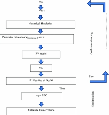
The schematic of FIA loop for LBO prediction is plotted in Fig. 1. The procedure of LBO prediction using FIA(Reference Hu, Huang and Wang32) is briefly described below:
-
1. Set the initial fuel mass flow rate mf,0 and then solve the velocity and concentration field of the combustor without combustion.
-
2. Based on the computational results obtained in Step 1, V flammable,0 could be determined by the fuel lean flammable limit, which can be obtained from a NIST-JANAF (National Institute of Standards and Technology–Joint Army, Navy and Air Force) table or calculated from incoming conditions for other nonstandard conditions. α could be directly obtained by the mass flow integral.
-
3. A new fuel mass flow rate (mf,1) can be obtained by substituting V flammable,0 and α into Equation (3). If |mf, n−mf, n−1|/mf, n < σ, the results are convergent and the iteration is stopped. mf,n is considered to be the fuel mass flow rate at LBO. Otherwise, reset the fuel mass flow rate in numerical simulation as mf,1 and repeat Step 1.
Schematic of extended FIA for flame volume prediction.

Once the V flammable is determined, the air involved in the V flammable can be obtained easily by numerical simulations. V flammable is defined according to the lean/rich limits. Cold simulation only provides the information about the flammable mixture contour in the solution domain, and does not have any information about flame or high-temperature regions. Hence, V flammable is bridged to Vf by a liner fit that is based on experimental data, as shown in Equation (4). The multiplication factor of 140 reflects the fact that V flammable is very small in comparison to the actual flame volume and points towards a possible margin for improvement. The underprediction of flammable volume is associated with built-in modelling deficiencies of cold flow simulations. To overcome this limitation, improvement is suggested in the prediction methodology.
 $$\begin{equation}
{V_f} = 140{V_{{\rm{flammable}}}} - 0.0002
\end{equation}$$
2.2 Hot flow physics
Previously, the FIA prediction methodology depended on cold flow simulations. However, studies suggest that flow physics in the recirculation region (IRZ) is quite different in reacting and non-reacting cases, which provides another basis for conducting hot simulations. Multiple comparative studies(Reference Gabruk and Roe33-Reference Ezhil and Mishra35) of hot and cold flow fields have been conducted in the recirculation region of combustors. All of them suggest observable large-scale difference between recirculation regions of cold and hot flow fields. The main differences include: a) combustion length decreases approximated 50%(Reference Gabruk and Roe33), b) maximum reverse flow point is at 30% (60% in cold flow) of the recirculation zone length, c) a stronger flow reversal, d) a lower maximum value of reverse mass flow rate, e) significantly low density, f) absence of a large-scale mixing mechanism, and g) volumetric expansion due to heat release. The overall reduction of recirculation zone at such a large scale, as well as local axial and radial velocity increases due to heat release and volumetric expansion, would definitely affect the flame volume and structure. For these reasons, the authors believe that integrating reactive flow physics in the prediction loop would not only make it a more generalised model but would also increase the prediction accuracy and provide more insight into the flow physics. Hence, a reactive flow simulation has been carried out, but with simple combustion models to maintain the robustness.
2.3 Reactive flow simulation
It is anticipated that extension of a cold flow simulation to a reactive flow simulation will provide two advantages:
-
• The prediction loop will no longer depend on Equation (4) and will provide a realistic value of Vf from simulation.
-
• The inclusion of a hot simulation will improve the prediction methodology based on differences of physics between hot and cold flows.
To maintain the robustness in the prediction loop, reactive flow simulations were carried out with a non-premixed combustion model available in Fluent 15.0. The criterion to define flame in the solution domain was established. The pivotal parameters were identified, and their influence on the set-up reactive flow simulation was analysed. This criterion would be suitable for all the combustors operating in the vicinity of lean blow-out limits with similar inlet boundary conditions. The flame volume criterion is validated against test results of 11 different combustors.
3.0 COMPUTATIONAL METHODOLOGY
3.1 Geometric configurations
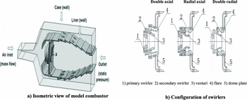
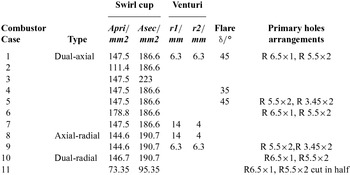
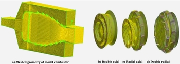
To maintain the generality in flame volume estimation methodology from reactive flow simulation, 11 combustor geometries were investigated. A typical combustor has four components: swirlers, venturi, flares and primary holes. Three liner configurations and swirler types (double axial, double radial and axial radial) were selected. Similarly, two geometric combinations of flare and venturi were embedded in the study. These geometric variations were incorporated to maintain the prediction methodology reliable and universal. The dome height (92 mm), liner length (226 mm) and combustor volume (0.00129 m3) were kept constant for the entire range of combustor configurations. An isometric view of the model combustor is shown in Fig. 2 and geometric configuration details are provided in Table 1.
Schematic of model combustor and swirl cups.

Combustor configurations and geometric parameters

3.2 Non-premixed model
To maintain the robustness in hybrid methodology, a non-premixed model (available in Fluent) was employed. In a non-premixed modelling approach, instantaneous thermochemical states of the fluid are related to the conserved scalar quantity known as mixture fraction (f)(Reference Sivathanu and Faeth36) as shown in Equation (5). The combustion process is simplified to a mixing problem in a mixture fraction approach. The Favre mean (density-averaged) mixture fraction equation is shown Equation (6).
 $$\begin{equation}
f = \frac{{{Z_i} - {Z_{i,ox}}}}{{{Z_{i,{\rm{fuel}}}} - {Z_{i,ox}}}}
\end{equation}$$
 $$\begin{equation}
\frac{\partial }{{\partial t}}\left( {\rho \bar{f}} \right) + \nabla .\left( {\rho \bar{v}\bar{f}} \right) = \nabla .\left( {\frac{{{\mu _l} + {\mu _t}}}{{{\sigma _t}}}} \right) + {S_m}
\end{equation}$$
The instantaneous scalars were related to averaged values by an assumed probability density function (PDF) as its closure. The shape of assumed PDF was described by double delta function as shown in Equation (7). A PDF table was generated with 20 species (C12H23, CO, CO2, H2O, N2, CH4, etc.)
 $$\begin{equation}
p\left( f \right) = \left\{ {\begin{array}{@{}*{2}{c}@{}} {0.5,}&{f = \bar{f} - \sqrt {\overline {{f^{'2}}} } }\\ {0.5,}&{ = \bar{f} + \sqrt {\overline {{f^{'2}}} } }\\ {0,}&{{\rm{elsewhere}}} \end{array}} \right\}
\end{equation}$$
3.3 DPM model
Standard aviation fuel, RP-3(C12H23), was selected for simulation. Air was treated as continuous phase and liquid fuel injection was modelled by a discrete phase model (DPM) that is based on a Lagrangian approach. Laws of heating, evaporation and boiling were applied for droplets. Heat transfer to a droplet was computed separately with Equation (8) and the mass of a droplet is reduced according to Equation (9). Stochastic tracking was used to keep the track of dispersing particles. The coupling between continuous and discrete phases was included and updated and performed after five iterations of continuous phase. The trajectory of discrete phase particle was predicted by force balance including drag force per unit particle as shown in Equation (10).
 $$\begin{equation}
{m_p}{c_p}\frac{{d{T_p}}}{{dt}} = h{A_p}\left( {{T_\infty } - {T_p}} \right) - \frac{{d{m_p}}}{{dt}}{h_{fg}},
\end{equation}$$
 $$\begin{equation}
{m_p}\left( {t + \Delta t} \right) = {m_p}\left( t \right) - {N_i}{A_p}{M_{w,i}}\Delta t,
\end{equation}$$
 $$\begin{equation}
F = \sum \left( {\frac{{18\mu {C_D}Re}}{{{\rho _p}d_p^224}}\left( {{u_p} - u} \right) + {F_{{\rm{other}}}}} \right)m_p^.\Delta t\ ,
\end{equation}$$
where mp
is the mass of particle, cp
is heat capacity, Ap
is surface area of particle, T
∞ is local temperature of continuous phase, Tp
is droplet temperature, h is convective heat transfer coefficient,
 $\frac{{d{m_p}}}{{dt}}$
is rate of evaporation, hfg
is latent heat. Ni
is molar flux of vapour, M
w, i
is molecular weight of species i, up
is particle velocity and CD
is drag coefficient.
3.4 Fuel injection
A hollow cone atomiser was placed at the injection coordinates (–220, –21, 0) and liquid fuel was injected through a slot of 0.79 mm diameter. Fuel flow rate corresponding to lean limit was set for each configuration based on experimental data. The injection temperature of the droplets was set as 300°K. Moreover, the injection velocity was estimated based on mass flow measurement and was 20 m/s, and the droplets were injected without any velocity fluctuations. Discrete random walk model was selected to track droplets. The boundary conditions for the liquid fuel were: (1) deterministic inlet velocity, injection angle and location (2); the droplets hitting walls were reflected and can escape from outlet boundary domain, and (3) 0.5 swirl. Additionally, the minimum droplet diameter was limited to 1 μm, and smaller droplets were regarded as evaporated. The maximum droplets temperature was limited to the boiling temperature for Kerosene, Tbn = 371°K. The Sauter mean diameter (SMD) of droplets varied from 10 to 30 µm to study its effects on Vf .
3.5 Thermodynamic properties
Thermodynamic properties for individual species and RP3 were defined by a NASA fifth-order piecewise polynomial. NASA polynomial parameterisations for specific heat capacity, enthalpy and entropy are shown in Equation (11)-(13) respectively. Mixture properties were calculated from individual species based on the mixing law.
 $$\begin{equation}
\frac{{c_p^0}}{R}\left( T \right) = {a_0} + {a_1}T + {a_2}{T^2} + {a_3}{T^3} + {a_4}{T^4},
\end{equation}$$
 $$\begin{equation}
\frac{{h_{}^0}}{R}\left( T \right) = {a_0} + \frac{{{a_1}}}{2}T + \frac{{{a_2}}}{3}{T^2} + \frac{{{a_3}}}{4}{T^3} + \frac{{{a_4}}}{5}{T^4} + \frac{{{a_5}}}{T},
\end{equation}$$
 $$\begin{equation}
\frac{{s_{}^0}}{R}\left( T \right) = {a_0}{\rm{ln}}\left( T \right) + {a_1}T + \frac{{{a_2}}}{2}{T^2} + \frac{{{a_3}}}{3}{T^3} + \frac{{{a_4}}}{4}{T^4} + {a_6},
\end{equation}$$
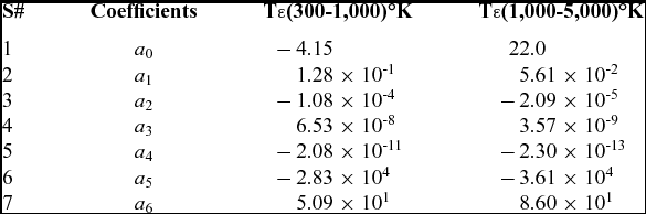
The superscript 0 denotes the reference state, c 0 p is the specific heat capacity at constant pressure, h 0 is the enthalpy and s 0 is the entropy. The coefficients ai for kerosene are given in Table 2.
Coefficients of the NASA polynomials for kerosene for two ranges of temperature (http://cea.grc.nasa.gov)

3.6 Turbulence model
Mongia(Reference Black and Smith26) conducted a detailed study on turbulence models; realisable k-ε offers better prediction capability to predict flows involving rotation, boundary layers, and strong adverse gradients, separation and recirculation. The equations for k and ε are:
 $$\begin{equation}
\frac{{\partial \left( {\rho k} \right)}}{{\partial t}} + \frac{{\partial \left( {\rho k{u_j}} \right)}}{{\partial {x_j}}} = \frac{{\partial \left[ {\left( {\mu + \frac{{{\mu _t}}}{{{\sigma _k}}}} \right)\frac{{\partial k}}{{\partial {x_j}}}} \right]}}{{\partial {x_j}}} + {G_k} + {G_b} - \rho \varepsilon - {Y_M} + {S_k},
\end{equation}$$
 $$\begin{equation}
\frac{{\partial \left( {\rho \varepsilon } \right)}}{{\partial t}} + \frac{{\partial \left( {\rho k{u_j}} \right)}}{{\partial {x_j}}} = \frac{{\partial \left[ {\left( {\mu + \frac{{{\mu _t}}}{{{\sigma _\varepsilon }}}} \right)\frac{{\partial \varepsilon }}{{\partial {x_j}}}} \right]}}{{\partial {x_j}}} + \rho {C_1}{S_\varepsilon } - \rho {C_2}\frac{{{\varepsilon ^2}}}{{k + \sqrt {v\varepsilon } }} + {C_{1\varepsilon}}\frac{\varepsilon }{k}{C_{3\varepsilon }}{G_b} + {S_\varepsilon },
\end{equation}$$
where Gk represents the generation of turbulence kinetic energy due to the mean velocity gradients. Gb is the generation of turbulence kinetic energy due to buoyancy. YM represents the contribution of the fluctuating dilatation in compressible turbulence to the overall dissipation rate. C 2 and C 1ε are constants, and set as 1.9 and 1.44, respectively. σk and σε are the turbulent Prandtl numbers for k and εand are set as 1.0 and 1.2, respectively.
3.7 Boundary conditions
The inlet static temperature (300°K) and total pressure (256 Kpa) was defined for the incoming air at inlet boundary. The outlet boundary pressure (101 Kpa) condition was maintained with target mass flow rate to ensure the air mass flow rate (0.51 kg/s). The wall was considered as non-adiabatic with no slip. The turbulence property at the combustor inlet was characterised by turbulence intensity (10%) and turbulence length scale (DH=4Ac/Cw=36.34 mm). Wall surfaces pose a ‘reflect’ boundary condition for DPM fluid. Escape DPM boundary has been defined at the inlet and outlet of the continuous phase. Standard wall function was utilised for near-wall treatment. The fuel flow rate set in numerical simulations was obtained from LBO experiments. To maintain the similarity in the tested model and simulated geometry, the periodic surfaces were declared as solid walls in simulation.
3.8 Grid generation and validation computation
Combustor geometry was preprocessed and meshed in GAMBIT 2.3.16 as shown in Fig. 3. Mesh was generated on 18-degree single sector with 3.5 million grid cells. Tetrahedral grids were generated in and around the dome and the liner. Other regions were generated in hexahedral grids. Second order upwind discretisation scheme was utilised for momentum, turbulent dissipation rate and turbulent kinetic energy equations. The Reynolds Average Navier–Stokes (RANS) calculation for combustion was conducted by using the commercial software Fluent 15.0 and further validated by the experimental results in the present study. RANS with the widely used Realisable k–e model was adopted in the present study based on the considerations that only time-average flow fields were considered and measured in the study. The solutions were performed on a Dell Precision 530 (twin Intel Xeon CPU having 2.4 GHz speed and 2G RAM) workstation. The approximate solution time for one simulation is three hours. Systematic work for validation of boundary conditions, grid generation, turbulent models and boundary condition on model combustor has been conducted by the author in an earlier study (Ref. Reference Hu, Huang, Wang and Xie37, pp 441-443) and is not discussed here.
Meshed computational domain.

4.0 EXPERIMENTAL SET-UP
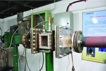
The LBO experiments were conducted on a single dome (1/18 of annular combustor) rectangular combustor model with optical access on one side wall. All the tests were conducted in the combustion test facility of Beihang University as shown in Fig. 4. Air flow was monitored until steady-state flow conditions were achieved. Afterwards, fuel was injected and ignited by spark plug, and the combustor was run in a stable regime (away from lean limit) for approximately 10 minutes to achieve thermal equilibrium. During the experiments, the injection pressure for fuel was maintained at 30 bar to ensure uniform droplet distribution for the entire range of experimentation. Then fuel flow rate was gradually decreased until LBO limit was achieved. The mass flow rates for fuel and air were recorded and video of the last 5 seconds was recorded with a high-speed camera. The frames were time-averaged to estimate flame volume. As the flame was captured from a side window, it provided a 2D profile. It was assumed that the obtained 2D image was axis-symmetric and revolution around the axis provides the flame volume. The measurement uncertainty in experiments was within ±4%. The detailed description of rig, errors analysis and Vf measurement can be found in Ref. Reference Xie, Huang, Wang and Hu30.
Experimental setup for LBO measurement.

5.0 RESULTS AND DISCUSSION
The
 $[ {\frac{{A\,{f_{{\rm{PZ}}}}}}{{{V_c}}}} ]$
term in Equation (1) represents effects of combustor geometry on q
LBO. It has been argued while proposing the flame volume model that the geometric parameter Vc
is lacking as a mathematical representation of the complex interaction of mixing jets associated with geometric configuration. The author believes that while presenting the LBO correlation based on Vc
, the researchers were aware of the following: Vf
is not always equal to Vc
, an inability of Vc
to represent the complex flow physics involved in IRZ, and intricacies attached with Vf
estimation. But they preferred Vc
over Vf
. The reason for the tradeoff between simplicity and accuracy was to have a rather simple and robust predictive correlation rather than a very accurate one, which can be utilised rigorously at the preliminary design stage. The approach was pragmatic and successfully produced the correlation fit for initial design stage but resulted in a compromised prediction accuracy. In the context of Vf
estimation, it is a challenging task either by a numerical approach or with high-tech optical diagnostic equipment. Developing the capability to retrieve 3D image flames in a practical combustor is a challenge for the experimentalist. It also demands a huge amount of time and financial resources for a single design iteration. In addition, experiments cannot commence prior to preliminary design, so experimental estimation cannot become part of any prediction tool. Hence, a better understanding of phenomena and its efficient incorporation in a mathematical arrangement could yield improvement. The improved empirical correlation in Equation (2) suggested by Huang(Reference Kim, Lienau, Van Slooten, Colket, Malecki and Syed18) include two geometric parameters, α and β (β =Vf
/V
c). This improvement has been carried out at the cost of complexity attached with Vf
estimation. Vf
is a strongly associated with and affected by local flow physics within primary zone and operating AFR, i.e., the throttle of the engine.
Several parameters affect the local flow physics: Swirl Number (SN), size of recirculation zone, the amount of recirculating flue gases, the geometry of the dome, the amount of air taking part in combustion, the penetration of air through primary holes, and location of the primary holes. Hence, Vf can be considered as a one lumped parameter representing the complex interdependence of the above-mentioned parameters. With the involvement of a large number of parameters and their complex interdependence, the pragmatic solution is to simulate the hot flow and get the holistic view in terms of flame volume. Hence, a reactive flow simulation with the simplest non-premixed combustion model to estimate flame volume and its calibration against experimental data could be a productive stride towards development of simple and robust predictive tool. Moreover, it will also enhance the understanding of combustion phenomena and would be beneficial for future studies.
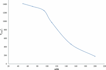
Apart from local flow physics, Vf is also dictated by AFR or engine throttle. As we move along the operating line of the engine from maximum to idle rpm, AFR value decreases (300-50 in the case of small engines) and as a consequence, Vf also decreases. From the plot of Vf versus engine operating line plotted in Fig. 5, it is evident that the combustor has maximum flame dimension (Vf ~Vc ) at max rpm and minimum (Vf ~Vc /5) in the vicinity of lean blow-out. It can be observed that the value of Vf reduces up to fourfold near q LBO and this value truly reflects the effect of the dome and primary zone configuration on LBO. Hence, Vf is a more appropriate and dynamic parameter representing local geometry and flow physics in comparison to the fixed geometric parameter Vc . Two vital parameters that influence the Vf identification in solution domain are critical temperature (T crit) and droplet nominal diameter (D p, crit).
Variation of Vf vs operating throttle of engine (AFR).

5.1 Flame identification and estimation methodology
T crit is the foremost important parameter; its critical value must be identified. Critical value of temperature means that anything above this value can be considered as a flame and this value will help define the Vf in the solution domain. The standard practice is to identify flame by OH contour plot, while in PDF models, all the scalar parameters are unique functions of the mixture fraction ‘f’ (∅ i = ∅ i (f)). Under the assumption of chemical equilibrium, all thermochemical scalars (including species fraction, density and temperature) depend solely on the instantaneous mixture fraction. Hence, temperature contour can be used as a marker for flame identification in numerical studies. As far as flame identification in real life is concerned, high-speed visualisation systems involving CCDs in the visible spectrum (VIS, 400-700 nm) are particularly suitable to determine flame shape, brightness and oscillation frequency, which are related to combustion efficiency and flame stability(Reference De Giorgi, Sciolti, Campilongo and Ficarella38). The acquisition of flame signature in visible region is easier and cheaper, especially for real aero engine combustors which offer limited optical access for experimentation. The visible emanating energy can be attributed to the spectra of electronically excited combustion radicals CH (430 nm) and C2 (473.71 nm and 516.52 nm), and can be captured by CCDs operating in visible spectral range.
After performing the reactive flow simulation, a series of section planes normal to the Z axis were generated and the temperature contour was plotted. The gap between any two neighbouring cut planes was set to be 5 mm and a total of 17 Z-planes were generated. They were then assembled in the XY plane by deleting Z the coordinate. The threshold value of temperature was declared as critical temperature (T crit) and any value below than T crit was clipped off from the solution domain to get flame. The boundary was defined in Tecplot and subsequent surface integrals provided the flame area. This flame was rotated around the axis of symmetry to calculate Vf . This approach provided the exact similarity between the experimental and simulated procedure for Vf estimation.
5.2 Minimum flame temperature
Unfortunately, most of the published literature discusses either peak or adiabatic temperature in flames, which is not valuable for flame identification in the present study. For identification, it is necessary to define a threshold value of temperature that can be used as flame marker and requires calibration against experimental data. As all LBO experiments were conducted under atmospheric pressure and ambient temperature, an analogy in temperature flow field exists between LBO experiment and open fires. Some literature focused on minimum temperatures within open fires can be found in the late 1990s. McCaffrey(Reference McCaffrey39) divided open flame into three different regimes: a) continuous flame region where the temperature range is 900-1,250°C, b) intermittent flame region where flame tips sheds off like a Von Kármán vortex and the plume moves upwards, c) flame tip/thermal plume region where the flame is not visible and the temperature continually drops down the stream. The intermittent flame region is the visible flame tip region that has to be identified for Vf measurement. McCaffrey and Chitty's studies show 613°K for the region b. Cox(Reference Smith and Cox40,Reference Cox and Chitty41) found out that for higher heat release rate fires, the threshold value is around 823°K. Ingason(Reference Ingason42) adopted the criteria of a range covering 573-873°K, while Heskestad(Reference Heskestad43) selected 773°K. A study on LES of pool fires(Reference Kang and Wen44) suggest that visible flame boundaries are indicated by a temperature of 600°K. To identify flames within the solution domain, the most important thing is the threshold value of temperature above which the entire region can be declared as flame. The studies carried out by various researches in Refs Reference McCaffrey39-Reference Kang and Wen44 provided a clue that threshold temperature (T crit) is in the range of 573-873°K for a less intense fire. However, the fire in a gas turbine combustor is more intense than in open fires, so a higher value for T crit could be envisaged. The AFR value at LBO limits for respective geometric configuration is shown in Table 3.
AFR value at lean blow-out limit for combustors

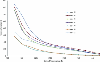
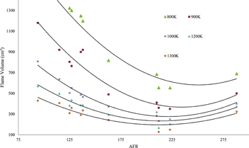
Reactive flow simulations for 11 combustor configurations were conducted at their respective LBO conditions rate and Vf calculated. Figure 6 presents variation in estimation of Vf at LBO conditions against T crit selection. It is obvious that against low values (e.g., 900°K) of T crit, flame volume is greater and vice versa. But the important inference is that even though Vc is kept constant for entire range of combustor configurations, Vf holds a unique value for each configuration, no matter what value of Tcrit (800-1,300°K) is selected. However, this uniqueness is more distinct for lower values and fades away for higher values of T crit. That is logical, as high-temperature regions are small in size and are indifferent to geometric configurations. This demonstrates that flame volume is a better parameter to pick up the effect of geometric configuration against Vc , and defining T crit in the range of 800-1,200°K would be more beneficial.
Vf vs different selected values of T crit.

In Fig. 7, flame volumes estimated for each configuration against five selected values of T crit (800, 900, 1000, 1,200 and 1,300°K) are presented. Each geometric configuration can be traced against its AFR given in Table 3. The ability of Vf to pick up the effects of geometry decreases against higher value of T crit and is more distinct vice versa. Geometries possessing large flame volumes at their lean limit blow out at smaller values of AFR, i.e., configurations 2 and 4 (q LBO~115 & 94). On the other hand, geometries with a small flame volume at the lean limit are more stable and show more endurance, and they blow out at larger values of AFR, i.e., configurations 8 and 9 (q LBO~250). This is in line with experimental observations and refers to the inference that large flame volumes with better mixing discourage local fuel-rich regions which are necessary to keep the combustor lit.
Variation of Vf against five selected values of T crit.

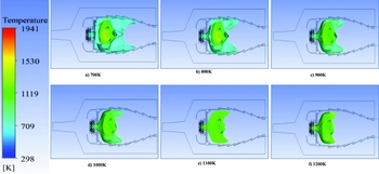
For configuration 01, the probable flame shape against temperature range from 700°K to 1,200°K is shown in Fig. 8. It is evident that high-temperature regions are enveloped by low-temperature contours and the highest temperature region lie at IRZ. Hence selection of T crit has vital impact on flame volume estimation.
Iso-surface at different T crit for configuration 1.

5.3 Droplet diameter
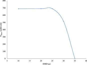
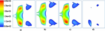
The second most influential parameter on Vf is the SMD of atomising fuel. The effect of injection diameter was studied by varying the value of D P from 10 to 35 μm. Vf is defined by T crit=900°K. It can be seen in Fig. 9 that Vf remains almost unchanged up till a threshold value of about 25 μm and then suddenly drops to zero with a small increment of 5 μm. This threshold value of droplet size is termed as D p,crit and presents the difference between evaporation and mixing controlled combustion. If the droplets of D p < 25 μm were injected, 100% of the fuel evaporates within IRZ and becomes part of the continuous flow field; hence, mixing controlled combustion prevails. Figure 10 presents the pictorial view for 10, 20, 25 and 30 μm droplets. All the droplets less than 25 μm were evaporated well before the end of primary zone. In this case, evaporation time scales appear to be small and play no controlling part in overall combustion process. The temperature contour plotted in Fig. 11 exhibits a similar behaviour for D p < 30 μm. For D p > 30 μm, it was observed fuel is not fully evaporated and some portion of it leave IRZ unevaporated. Consequently, a sudden decrease in Vf was observed. When the temperature contour plot was clipped off for all values less than 900°K as shown in Fig. 12, it was seen that Vf is unchanged up to 25 μm but exhibits no flame for 30 μm droplets.
Effect of injection D p on Vf .

Effect of D p on penetration length and evaporation time.

Variation in temperature flow field against injection D p.

Temperature contour plot for T crit > 900 presenting flame volume variation vs injection D p.

The phenomenon can be rationalised thus: when all droplets are evaporated within the recirculation zone, the flow physics, which is constant for one selected combustor configuration, dictates the flame volume. In other words, we may say that for mixing controlled combustion (D p < D p, crit), flame volume is only a function of combustor geometric features. Once the droplet diameter (D p < D p, crit) exceeds the critical value, it switches the evaporation mechanism into a controlling phenomenon, in this case flame volume = f (combustor geometry, D p).
5.4 Criterion for flame volume
The systematic study of T crit and D p,crit led to the identification of flame with in solution domain and is based on two inferences: (1) flame volume is in sensitive to droplet injection diameter for D p <25 µ (mixing controlled combustion prevails), (2) flame volume estimation for different value of T crit (1,300°K, 1,200°K, 1,000°K, 900°K and 800°K) shows that a close match exists with experimental data against T crit = 900°K. This generalised flame identification criterion is valid for all kerosene-fueled combustors, provided combustion that mixes controlled and reactants are fed at ambient conditions.
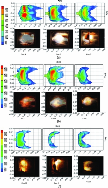
Based on the laid-down criterion for flame identification, flame profiles were estimated by reactive flow simulations. Their comparison with the time-averaged experimental snapshots would help to judge the efficacy of the flame identification criterion. Figure 13 presents a comparison between the estimated flame shape and experimental snapshots. The flame profile, in solution domain, was extracted by the procedure described in section VI-A. The injector location is x = –0.22 m and y = –0.02. The black zone in the images of combustors 2, 5, and 13 is due to deposition of coke generated by kerosene sprayed to the quartz windows. The vertical line visible at x = 0.15 m is a cooling slit in the inner quartz window. The snaps were arranged form higher AFR to lower. The maximum flame size exits can be seen in Fig. 13 (case 4) and the minimum in Fig. 13 (case 8).
Comparison between snapshot and estimated flame profile by reactive flow simulation.
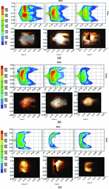
Based on the flame identification criterion in the solution domain, the captured flame shapes exhibit a close match with their respective experimental snapshots. Figure 13 also indicates that the flame shape is closely related to the swirler configuration. The subcaptions in Fig. 13 correspond to the combustor case number as mentioned in Table 01. Combustors with dual-axial swirlers (Fig. 13, cases 1-7), owing to the large axial momentum, exhibit longer flames, and the edges of the flame regions protrude to the downstream. In the combustors assembled with axial-radial or dual-radial swirlers (Fig. 13, cases 8-10), due to presence of radial momentum, flames are wider but shorter in length. In Fig. 13 (case 5), the edges of flames reach to –0.09 m, which is in agreement with experimental snapshot. The width of flame is from –0.06 to 0.02 and was well captured by the estimation methodology. Both lifted and attached types of flames were captured by the simulation. The lifted flame could be seen in Fig. 13 (case 9) and was well captured by the simulation. Similarly Fig. 13 (case 7) presents close matching between experimental and estimated flame volumes. According to the projected area from the side view of the flame region, Vf obtained by numerical simulation fits well with that obtained by experiment. The flame length and width are two important parameters that are closely linked with dome geometry, and they exhibit close similarity with the experimental profile. It shows that the laid-down criterion is capable of Vf estimation and holds a great potential for utilisation in LBO estimation. Moreover, the flame region obtained either by numerical simulations or experiments cannot encompass the whole combustor. It varies from case to case depending on dome geometry and holds a small region located close to the atomiser that is inconsistent with the combustion volume definition contained in Lefebvre's original model.
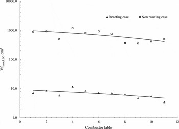
In the previous study(Reference Hu, Huang and Wang32), only cold flow simulations were carried out and flame volume was estimated by identifying flammable concentration contours in the solution domain. The resultant flammable volume, estimated by subtracting the volume encapsulated by rich flammability limit from lean flammability, was underestimated by the factor of 140. Hence, Equation (4) must be used for correction. Figure 14 presents a comparison of flame volume estimated from reactive flow simulation and cold flow simulation. The logarithmic coordinate is adopted for the y axis to demonstrate the comparison more clearly. The difference between reactive and nonreactive flow physics is the core reason behind this difference. With the inclusion of reactive flow simulation, more realistic flame estimation has become possible. Moreover, the gap between flammable volume and flame volume has been successfully bridged, and dependence on Equation (4) has been eliminated from the prediction loop. This will be very advantageous when will be embedded in the prediction loop for LBO estimation.
Comparison of Vf obtained from reacting flows and non-reacting flows.

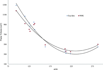
Figure 15 shows a close match between estimated Vf' and experimental measured value for entire range of combustor configurations. Each point refers to flame volume for each configuration at its respective LBO limit. The maximum error with experimental data is ±15%. The criteria for identification of flame and no flame region also hold similarity with the previous work Refs Reference McCaffrey39-Reference Kang and Wen44. 900°K contour exhibits the best match with our experimental data also. The matching accuracy is very encouraging and holds a promising improvement in LBO prediction. In future, research orientation will be towards prediction of q LBO based on this Vf criterion established here.
Comparison of estimated vs. experimentally measured V f.

6.0 CONCLUSIONS
-
1. In the context of FV-LBO prediction, reactive flow simulations for 11 combustor geometries have been carried out. The general criterion for Vf estimation in solution domain has been established. This study bridges the gap between flammable volume and flame volume, and dependence on Equation (4) has been eliminated. Now Vf can be estimated directly from a hot simulation.
-
2. Reactive flow simulation with the combination of PDF and DPM models, which are able to predict Vf with ±85% accuracy, have enhanced the capability and universality of the FV-LBO model. T crit and D p,crit have been identified as the two most significant parameters in Vf prediction simulation.
-
3. The benchmarking of T crit has been done successfully and it has been inferred that a temperature contour at 900°K best matches with the experimental value of Vf .
-
4. D p,crit is identified as a threshold injection droplet diameter, injecting D p < D p,crit will have no effect on Vf and mixing controlled combustion prevails. If D p > D p,crit is injected, evaporation-controlled combustion takes over; Vf becomes dependent on D p apart from combustor geometric configuration. Successful estimation of Vf with simple combustion models will enhance the predictive accuracy of hybrid methodology (FV-LBO) without losing the robustness.
ACKNOWLEDGEMENTS
This work was carried out with the help of Hu Bin, who is presently serving at the Institute of Engineering Thermophysics at the Chinese Academy of Science. The authors would like to thank him for valuable advice and counselling.