3.1 Problem formulation

3.1.1 Governing equations for the mean flow and coherent fluctuations

We start from the Navier–Stokes equations

(3.1) $$\begin{eqnarray}\unicode[STIX]{x2202}_{t}\boldsymbol{U}+\boldsymbol{N}(\boldsymbol{U})=\boldsymbol{F},\end{eqnarray}$$

governing the dynamics of velocity $\boldsymbol{U}(\boldsymbol{x},t)$ and pressure $P(\boldsymbol{x},t)$ , where

(3.2) $$\begin{eqnarray}\boldsymbol{N}(\boldsymbol{U})=(\boldsymbol{U}\boldsymbol{\cdot }\unicode[STIX]{x1D735})\boldsymbol{U}+\frac{1}{\unicode[STIX]{x1D70C}}\unicode[STIX]{x1D735}P-\unicode[STIX]{x1D708}\unicode[STIX]{x1D6FB}^{2}\boldsymbol{U}\end{eqnarray}$$

is the nonlinear incompressible Navier–Stokes operator and $\unicode[STIX]{x1D70C}$ the fluid density. In this study we restrict our attention to incompressible flows since the Mach number is small, but the spirit of the derivation is similar for compressible flows. Hereafter, we therefore omit the continuity equation $\unicode[STIX]{x1D735}\boldsymbol{\cdot }\boldsymbol{U}=0$ . The term $\boldsymbol{F}(\boldsymbol{x},t)$ denotes a space- and time-dependent forcing applied either at a boundary or inside the domain. Following Reynolds & Hussain (Reference Reynolds and Hussain1972), the flow is decomposed into its time-averaged component $\overline{\boldsymbol{U}}(\boldsymbol{x})$ , coherent fluctuations $\widetilde{\boldsymbol{u}}(\boldsymbol{x},t)$ and turbulent fluctuations $\boldsymbol{u}^{\prime }(\boldsymbol{x},t)$ :

(3.3) $$\begin{eqnarray}\boldsymbol{U}=\overline{\boldsymbol{U}}+\widetilde{\boldsymbol{u}}+\boldsymbol{u}^{\prime }.\end{eqnarray}$$

By construction, time averaging ( $\overline{\,\cdot \,}$ ) yields the steady mean flow $\overline{\boldsymbol{U}}$ and removes all fluctuations ( $\overline{\widetilde{\boldsymbol{u}}+\boldsymbol{u}^{\prime }}=\mathbf{0}$ ), while phase averaging ( $\langle \cdot \rangle$ ) removes incoherent fluctuations ( $\langle \boldsymbol{U}\rangle =\overline{\boldsymbol{U}}+\widetilde{\boldsymbol{u}}$ , $\langle \boldsymbol{u}^{\prime }\rangle =\mathbf{0}$ ). Similar notations are used for other quantities, e.g. pressure, forcing and spanwise vorticity. Substituting this decomposition into (3.1) yields coupled equations for the mean flow and coherent fluctuations:

(3.4a ) $$\begin{eqnarray}\displaystyle & \boldsymbol{N}(\overline{\boldsymbol{U}})=-\unicode[STIX]{x1D735}\boldsymbol{\cdot }(\overline{\widetilde{\boldsymbol{u}}\widetilde{\boldsymbol{u}}}+\overline{\boldsymbol{u}^{\prime }\boldsymbol{u}^{\prime }})+\overline{\boldsymbol{F}}, & \displaystyle\end{eqnarray}$$

(3.4b ) $$\begin{eqnarray}\displaystyle & \unicode[STIX]{x2202}_{t}\widetilde{\boldsymbol{u}}+\boldsymbol{L}(\overline{\boldsymbol{U}})\widetilde{\boldsymbol{u}}=-\unicode[STIX]{x1D735}\boldsymbol{\cdot }(\widetilde{\widetilde{\boldsymbol{u}}\widetilde{\boldsymbol{u}}}+\widetilde{\boldsymbol{u}^{\prime }\boldsymbol{u}^{\prime }})+\widetilde{\boldsymbol{f}}, & \displaystyle\end{eqnarray}$$

where $\boldsymbol{L}(\overline{\boldsymbol{U}})$ is the Navier–Stokes operator linearised around the mean flow,

(3.5) $$\begin{eqnarray}\boldsymbol{L}(\overline{\boldsymbol{U}})\widetilde{\boldsymbol{u}}=(\overline{\boldsymbol{U}}\boldsymbol{\cdot }\unicode[STIX]{x1D735})\widetilde{\boldsymbol{u}}+(\widetilde{\boldsymbol{u}}\boldsymbol{\cdot }\unicode[STIX]{x1D735})\overline{\boldsymbol{U}}+\frac{1}{\unicode[STIX]{x1D70C}}\unicode[STIX]{x1D735}\widetilde{p}-\unicode[STIX]{x1D708}\unicode[STIX]{x1D6FB}^{2}\widetilde{\boldsymbol{u}}.\end{eqnarray}$$

Equation (3.4) shows that, due to the forcing from the coherent and turbulent Reynolds stresses $\widetilde{\boldsymbol{u}}\widetilde{\boldsymbol{u}}+\boldsymbol{u}^{\prime }\boldsymbol{u}^{\prime }$ , the mean flow $\overline{\boldsymbol{U}}$ differs from the steady base flow $\boldsymbol{U}_{b}$ , which is a solution of the stationary Navier–Stokes equations $\boldsymbol{N}(\boldsymbol{U}_{b})=\overline{\boldsymbol{F}}$ .

Focusing on a coherent time-harmonic forcing at frequency $\unicode[STIX]{x1D714}_{1}$ ,

(3.6a-c ) $$\begin{eqnarray}\overline{\boldsymbol{F}}=\mathbf{0},\quad \widetilde{\boldsymbol{f}}(\boldsymbol{x},t)=\widetilde{\boldsymbol{f}}_{1}(\boldsymbol{x})\text{e}^{\text{i}\unicode[STIX]{x1D714}_{1}t}+\text{c.c.},\quad \boldsymbol{f}^{\prime }=\mathbf{0},\end{eqnarray}$$

where c.c. stands for complex conjugate, the coherent response is assumed to fluctuate at the forcing frequency and higher harmonics:

(3.7) $$\begin{eqnarray}\widetilde{\boldsymbol{u}}(\boldsymbol{x},t)=\mathop{\sum }_{n\neq 0}\widetilde{\boldsymbol{u}}_{n}(\boldsymbol{x})\text{e}^{\text{i}n\unicode[STIX]{x1D714}_{1}t}=\mathop{\sum }_{n>0}\widetilde{\boldsymbol{u}}_{n}(\boldsymbol{x})\text{e}^{\text{i}n\unicode[STIX]{x1D714}_{1}t}+\text{c.c.}\quad (\widetilde{\boldsymbol{u}}_{-n}=\widetilde{\boldsymbol{u}}_{n}^{\ast }).\end{eqnarray}$$

Introducing this Fourier decomposition into (3.4) yields an infinite system of equations for the mean flow $\overline{\boldsymbol{U}}$ and each coherent fluctuation  $\widetilde{\boldsymbol{u}}_{n}$ :

(3.8a ) $$\begin{eqnarray}\displaystyle & \displaystyle \boldsymbol{N}(\overline{\boldsymbol{U}})=-\mathop{\sum }_{n\neq 0}\unicode[STIX]{x1D735}\boldsymbol{\cdot }\widetilde{\boldsymbol{u}}_{n}\widetilde{\boldsymbol{u}}_{-n}-\unicode[STIX]{x1D735}\boldsymbol{\cdot }\overline{\boldsymbol{u}^{\prime }\boldsymbol{u}^{\prime }}, & \displaystyle\end{eqnarray}$$

(3.8b ) $$\begin{eqnarray}\displaystyle & \displaystyle \text{i}n\unicode[STIX]{x1D714}_{1}\widetilde{\boldsymbol{u}}_{n}+\boldsymbol{L}(\overline{\boldsymbol{U}})\widetilde{\boldsymbol{u}}_{n}=-\mathop{\sum }_{m\neq n,0}\unicode[STIX]{x1D735}\boldsymbol{\cdot }\widetilde{\boldsymbol{u}}_{m}\widetilde{\boldsymbol{u}}_{n-m}-\unicode[STIX]{x1D735}\boldsymbol{\cdot }(\widetilde{\boldsymbol{u}^{\prime }\boldsymbol{u}^{\prime }})_{n}+\unicode[STIX]{x1D6FF}_{n1}\,\widetilde{\boldsymbol{f}}_{1}, & \displaystyle\end{eqnarray}$$

where $(\widetilde{\boldsymbol{u}^{\prime }\boldsymbol{u}^{\prime }})_{n}$ denotes the coherent component at frequency $n\unicode[STIX]{x1D714}_{1}$ of the turbulent Reynolds stresses, and $\unicode[STIX]{x1D6FF}_{n1}$ is the Kronecker delta (equal to 1 if $n=1$ , and to 0 otherwise). For instance, the mean flow and first two harmonics are governed by

(3.9a ) $$\begin{eqnarray}\displaystyle & \boldsymbol{N}(\overline{\boldsymbol{U}})=-(\widetilde{\unicode[STIX]{x1D74D}}_{1,-1}+\widetilde{\unicode[STIX]{x1D74D}}_{2,-2}+\cdots \,)-\unicode[STIX]{x1D735}\boldsymbol{\cdot }\overline{\boldsymbol{u}^{\prime }\boldsymbol{u}^{\prime }}, & \displaystyle\end{eqnarray}$$

(3.9b ) $$\begin{eqnarray}\displaystyle & (\text{i}\unicode[STIX]{x1D714}_{1}+\boldsymbol{L}(\overline{\boldsymbol{U}}))\widetilde{\boldsymbol{u}}_{1}=-(\widetilde{\unicode[STIX]{x1D74D}}_{2,-1}+\widetilde{\unicode[STIX]{x1D74D}}_{3,-2}+\cdots \,)-\unicode[STIX]{x1D735}\boldsymbol{\cdot }(\widetilde{\boldsymbol{u}^{\prime }\boldsymbol{u}^{\prime }})_{1}+\widetilde{\boldsymbol{f}}_{1}, & \displaystyle\end{eqnarray}$$

(3.9c ) $$\begin{eqnarray}\displaystyle & (2\text{i}\unicode[STIX]{x1D714}_{1}+\boldsymbol{L}(\overline{\boldsymbol{U}}))\widetilde{\boldsymbol{u}}_{2}=-(\widetilde{\unicode[STIX]{x1D74D}}_{1,1}+\widetilde{\unicode[STIX]{x1D74D}}_{3,-1}+\cdots \,)-\unicode[STIX]{x1D735}\boldsymbol{\cdot }(\widetilde{\boldsymbol{u}^{\prime }\boldsymbol{u}^{\prime }})_{2}, & \displaystyle\end{eqnarray}$$

where we have introduced the notation

(3.10a,b ) $$\begin{eqnarray}\widetilde{\unicode[STIX]{x1D74D}}_{j,k}=\unicode[STIX]{x1D735}\boldsymbol{\cdot }\widetilde{\boldsymbol{u}}_{j}\widetilde{\boldsymbol{u}}_{k}+\text{c.c.}\quad \text{if}~j\neq k,\quad \widetilde{\unicode[STIX]{x1D74D}}_{j,j}=\unicode[STIX]{x1D735}\boldsymbol{\cdot }\widetilde{\boldsymbol{u}}_{j}\widetilde{\boldsymbol{u}}_{j},\end{eqnarray}$$

for the divergence of the coherent Reynolds stresses. At this stage no assumption has been made, other than the response fluctuates at $\unicode[STIX]{x1D714}_{1}$ and higher harmonics; the model is therefore general except for flows exhibiting other frequencies (for instance, subharmonics that appear via vortex pairing in some jets and mixing layers).

3.1.2 Turbulent viscosity

The effect of the unknown turbulent Reynolds stresses $\boldsymbol{u}^{\prime }\boldsymbol{u}^{\prime }$ on coherent fluctuations in (3.8) is accounted for with a turbulence model that relates $\widetilde{\boldsymbol{u}^{\prime }\boldsymbol{u}^{\prime }}$ to $\widetilde{\boldsymbol{u}}$ via a turbulent viscosity $\unicode[STIX]{x1D708}_{t}$ , such that (3.9) becomes

(3.11) $$\begin{eqnarray}(\text{i}\unicode[STIX]{x1D714}_{1}+\boldsymbol{L}(\overline{\boldsymbol{U}}))\widetilde{\boldsymbol{u}}_{1}=-(\widetilde{\unicode[STIX]{x1D74D}}_{2,-1}+\widetilde{\unicode[STIX]{x1D74D}}_{3,-2}+\cdots \,)+\widetilde{\boldsymbol{f}}_{1},\end{eqnarray}$$

where $\boldsymbol{L}$ now contains the modified viscosity $\unicode[STIX]{x1D708}+\unicode[STIX]{x1D708}_{t}$ . Specifically, we use a classical eddy viscosity model. The unknown coherent component of the turbulent Reynolds stresses $\widetilde{\boldsymbol{u}^{\prime }\boldsymbol{u}^{\prime }}$ is assumed to be proportional to the coherent strain rate $\widetilde{\unicode[STIX]{x1D64E}}=(\unicode[STIX]{x1D735}\widetilde{\boldsymbol{u}}+\unicode[STIX]{x1D735}\widetilde{\boldsymbol{u}}^{\text{T}})/2$ (Boussinesq approximation):

(3.12) $$\begin{eqnarray}\widetilde{\boldsymbol{u}^{\prime }\boldsymbol{u}^{\prime }}-{\textstyle \frac{2}{3}}\widetilde{q}\unicode[STIX]{x1D644}=-2\unicode[STIX]{x1D708}_{t}\widetilde{\unicode[STIX]{x1D64E}},\end{eqnarray}$$

where $\widetilde{q}=\widetilde{\boldsymbol{u}^{\prime }\boldsymbol{\cdot }\boldsymbol{u}^{\prime }}/2$ is the kinetic energy and $\unicode[STIX]{x1D644}$ the identity tensor. In this study the turbulent viscosity $\unicode[STIX]{x1D708}_{t}$ is taken as space-dependent, and calculated at each location according to

(3.13) $$\begin{eqnarray}\unicode[STIX]{x1D708}_{t}(\boldsymbol{x})=-{\displaystyle \frac{\overline{\boldsymbol{u}^{\prime }\boldsymbol{u}^{\prime }}\boldsymbol{ : }\overline{\unicode[STIX]{x1D64E}}}{2\overline{\unicode[STIX]{x1D64E}}\boldsymbol{ : }\overline{\unicode[STIX]{x1D64E}}}},\end{eqnarray}$$

where $\boldsymbol{ : }$ denotes the Frobenius inner product. In other words, at each location $\unicode[STIX]{x1D708}_{t}$ can be seen as resulting from the least-squares minimisation of the overdetermined system of equations $\overline{\boldsymbol{u}^{\prime }\boldsymbol{u}^{\prime }}=-2\unicode[STIX]{x1D708}_{t}\overline{\unicode[STIX]{x1D64E}}$ .

As explained in Pope (Reference Pope2000), the above model is a twofold simplification: first, it assumes that turbulent quantities ( $\widetilde{\boldsymbol{u}^{\prime }\boldsymbol{u}^{\prime }}$ ) can be related to the coherent motion ( $\widetilde{\unicode[STIX]{x1D64E}}$ ); second, it assumes that this constitutive relation is specifically of the form (3.12), i.e. linear isotropic (directly analogous to the relation for the viscous stress in a Newtonian fluid). Although the turbulent viscosity hypothesis is incorrect in general, it has been found reasonable in many simple turbulent shear flows (round jet, mixing layer, channel flow, boundary layer) where the turbulent and coherent characteristics change relatively slowly, following the mean flow.

In (3.13) we have implicitly assumed that coherent fluctuations do not affect the turbulent viscosity, i.e. although it is possible to linearise the turbulent model itself (Meliga et al. Reference Meliga, Pujals and Serre2012; Mettot et al. Reference Mettot, Sipp and Bézard2014; Viola et al. Reference Viola, Iungo, Camarri, Porté-Agel and Gallaire2014), here we use a turbulence viscosity computed once and for all for each given mean flow.

The steady component of the turbulent Reynolds stresses $\overline{\boldsymbol{u}^{\prime }\boldsymbol{u}^{\prime }}$ and the mean strain rate $\overline{\unicode[STIX]{x1D64E}}=(\unicode[STIX]{x1D735}\overline{\boldsymbol{U}}+\unicode[STIX]{x1D735}\overline{\boldsymbol{U}}^{\text{T}})/2$ are evaluated from the LES. It should be noted that $\overline{\unicode[STIX]{x1D64E}}$ is a direct output of the LES, whereas the calculation of $\overline{\boldsymbol{u}^{\prime }\boldsymbol{u}^{\prime }}$ requires further processing: indeed, the statistics of the total LES velocity field contain the steady component of both turbulent and coherent Reynolds stresses $\overline{\boldsymbol{u}^{\prime }\boldsymbol{u}^{\prime }}+\overline{\widetilde{\boldsymbol{u}}\widetilde{\boldsymbol{u}}}$ . This can be overlooked if the stresses $\overline{\widetilde{\boldsymbol{u}}\widetilde{\boldsymbol{u}}}$ are small compared to $\overline{\boldsymbol{u}^{\prime }\boldsymbol{u}^{\prime }}$ (Kitsios et al. Reference Kitsios, Cordier, Bonnet, Ooi and Soria2010; Viola et al. Reference Viola, Iungo, Camarri, Porté-Agel and Gallaire2014), which is not the case here because substantial coherent fluctuations are produced by the harmonic forcing in the large-amplitude regime. Therefore, before computing the turbulent viscosity, we first remove the coherent contribution $\overline{\widetilde{\boldsymbol{u}}_{1}\widetilde{\boldsymbol{u}}_{-1}}$ at the fundamental frequency, with $\widetilde{\boldsymbol{u}}_{\pm 1}$ obtained from frequency analysis. Specifically, coherent fluctuations $\widetilde{\boldsymbol{u}}_{1}$ from the 3D LES are computed by extracting 2D time-dependent velocity fields in the mid-plane $z=0$ , and performing a Fourier transform at the frequency of interest $\unicode[STIX]{x1D714}_{1}$ . Some authors have used an alternative approach based on energetic structures obtained from proper orthogonal decomposition (Tammisola & Juniper Reference Tammisola and Juniper2016) or have proposed weighting the turbulent viscosity by a laminar–turbulent intermittency factor (Oberleithner, Paschereit & Wygnanski Reference Oberleithner, Paschereit and Wygnanski2014).

3.1.3 Simplified model

In this paper, we wish to assess the possibility to capture correctly the amplification and saturation using a simplified model. We will compute coherent fluctuations at the frequency of interest $\unicode[STIX]{x1D714}_{1}$ via the linear response problem

(3.14) $$\begin{eqnarray}(\text{i}\unicode[STIX]{x1D714}_{1}+\boldsymbol{L}(\overline{\boldsymbol{U}}))\widetilde{\boldsymbol{u}}_{1}=\widetilde{\boldsymbol{f}}_{1}.\end{eqnarray}$$

In other words, we neglect nonlinear forcing terms $\widetilde{\unicode[STIX]{x1D74D}}_{j,1-j}$ arising from the interaction of coherent higher harmonics (even though those higher harmonics themselves, $\widetilde{\boldsymbol{u}}_{n}$ , $|n|\geqslant 2$ , may not be negligible), while we retain nonlinearities contained in the LES mean flow as well as nonlinearities involved in the turbulent viscosity. Put simply, we study the linearised dynamics of coherent fluctuations around (known) mean flows, with a turbulent viscosity model.

3.2 Numerical method

The 2D linear response to time-harmonic forcing is calculated around the mean flow obtained from LES (§ 2). The LNSE (3.14) are recast in variational form and discretised in domain  $I$ with the finite-element software FreeFem++ (Hecht Reference Hecht2012), using P2 and P1 Taylor–Hood elements for velocity and pressure, respectively (Boujo, Ehrenstein & Gallaire Reference Boujo, Ehrenstein and Gallaire2013; Boujo & Gallaire Reference Boujo and Gallaire2015). The 2D mesh contains approximately 330 000 triangular elements, strongly clustered in the mixing layer (see appendix A for a convergence study assessing the influence of the mesh size). Boundary conditions are as follows: $\widetilde{\boldsymbol{u}}_{1}=\mathbf{0}$ at the inlet $\unicode[STIX]{x1D6E4}_{in}$ and on the walls $\unicode[STIX]{x1D6E4}_{w}$ , stress-free condition $(1/\unicode[STIX]{x1D70C})\widetilde{p}_{1}\boldsymbol{n}+2(\unicode[STIX]{x1D708}+\unicode[STIX]{x1D708}_{t})\widetilde{\unicode[STIX]{x1D64E}}_{1}\boldsymbol{\cdot }\boldsymbol{n}=0$ at the outlet $\unicode[STIX]{x1D6E4}_{out}$ , and spatially uniform vertical forcing $\widetilde{\boldsymbol{u}}_{1}=v^{\prime }\boldsymbol{e}_{y}$ at the cavity end  $\unicode[STIX]{x1D6E4}_{f}$ .

3.3 Unforced case: linear stability analysis and linear harmonic response

Figure 3.

Global linear stability around the unforced mean flow ( $v^{\prime }=0$ ). (a) Eigenvalues lie on continuous branches, except marginally stable eigenvalues 1 and 2, which stand out at $\unicode[STIX]{x1D714}/2\unicode[STIX]{x03C0}=750$ and 1000 Hz. These two eigenvalues are not substantially affected by discarding turbulent viscosity (crosses). (b,c) Eigenmodes (unit norm; streamwise component, real part). Modes 1 and 2 are located in the shear layer and the downstream boundary layer, computed either with turbulent viscosity (‘TV’, panels b1, b2) or without (‘no TV’, panels c1, c2). (b3) Other modes are located inside the cavity.

We first focus on the unforced case, $v^{\prime }=0$ . Before moving on to the harmonic response problem, we investigate linear stability by solving the eigenvalue problem

(3.15) $$\begin{eqnarray}(\unicode[STIX]{x1D70E}+\text{i}\unicode[STIX]{x1D714})\widetilde{\boldsymbol{u}}+\boldsymbol{L}(\overline{\boldsymbol{U}})\widetilde{\boldsymbol{u}}=\mathbf{0}\end{eqnarray}$$

for infinitesimal perturbations $\widetilde{\boldsymbol{u}}$ around the LES mean flow  $\overline{\boldsymbol{U}}$ , with the numerical method as described in § 3.2. As shown in the spectrum in figure 3(a), all eigenmodes are stable (growth rate $\unicode[STIX]{x1D70E}\leqslant 0$ ). Most eigenvalues fall on continuous branches, and are more stable at larger frequencies. Two eigenmodes (denoted 1 and 2) stand out, however, at frequencies close to 750 and 1000 Hz, and are marginally stable (small growth rate compared to the angular frequency, $|\unicode[STIX]{x1D70E}|\ll \unicode[STIX]{x1D714}$ ). Marginal stability in mean flows has been observed in some laminar and turbulent flows, as well as counterexamples (Barkley Reference Barkley2006; Sipp & Lebedev Reference Sipp and Lebedev2007; Turton et al. Reference Turton, Tuckerman and Barkley2015; Meliga Reference Meliga2017). Here, modes 1 and 2 are located primarily around the downstream corner, as shown in figure 3(b1,b2). They are associated with spatio-temporal growth along the shear layer via the Kelvin–Helmholtz instability, decay in the downstream boundary layer, and feed back via a pressure wave from the downstream corner back to the upstream corner, reminiscent of leading eigenmodes observed in other cavities (Åkervik et al. Reference Åkervik, Hœpffner, Ehrenstein and Henningson2007; Sipp & Lebedev Reference Sipp and Lebedev2007; Barbagallo, Sipp & Schmid Reference Barbagallo, Sipp and Schmid2009). Modes 1 and 2 exhibit approximately one and two wavelengths across the cavity, respectively, i.e. smaller structures correspond to higher frequencies. Other modes are located inside the cavity, e.g. mode 3 in figure 3(b3). Discarding turbulent viscosity in the linear stability analysis (i.e. in $\boldsymbol{L}$ in the eigenvalue problem (3.15)) does not affect substantially eigenvalues 1 and 2 (black crosses in figure 3 a), and has a limited impact on the structure of modes 1 and 2 in the shear layer (figure 3 c1, c2).

Next, the linear response of the mean unforced flow to harmonic forcing on $\unicode[STIX]{x1D6E4}_{f}$ is characterised in terms of kinetic energy in domain  $I$ with the gain

(3.16) $$\begin{eqnarray}G(\unicode[STIX]{x1D714})={\displaystyle \frac{1}{v^{\prime }}}\left(\iint _{I}|\widetilde{\boldsymbol{u}}_{1}|^{2}\,\text{d}\boldsymbol{x}\right)^{1/2}.\end{eqnarray}$$

Figure 4(a) shows the gain obtained from the LNSE over a broad range of forcing frequencies (dashed line). The forcing is amplified preferentially in the frequency range 600–1200 Hz, with clear peaks close to 750 and 1000 Hz that can be related to the marginally stable modes 1 and 2.

3.4 Forced cases, saturation of the linear harmonic response

We now turn our attention to mean flows obtained from LES with harmonic forcing at $\unicode[STIX]{x1D714}_{1}/2\unicode[STIX]{x03C0}=750$  Hz, and recompute the linear response to harmonic forcing. In these mean flows, the gain consistently decreases with the forcing amplitude (solid lines in figure 4 a).

Figure 4.

(a) Linear harmonic gain $G(\unicode[STIX]{x1D714})$ of the turbulent mean flow forced at $\unicode[STIX]{x1D714}_{1}/2\unicode[STIX]{x03C0}=750$  Hz at different amplitudes  $v^{\prime }$ . Inset: $G(\unicode[STIX]{x1D714}_{1})$ in logarithmic scale (and a few results without turbulent viscosity shown as crosses). (b) Profiles of mean streamwise velocity  $\overline{U}$ .

In the following, we focus on the linear response to harmonic forcing at the frequency $\unicode[STIX]{x1D714}_{1}$ of the dominant peak. At this specific frequency (inset), the gain decreases by approximately one order of magnitude from the unforced regime to the large-amplitude forcing regime $v^{\prime }\gtrsim 2.5~\text{m}~\text{s}^{-1}$ . It should be noted that this effect comes entirely from the mean flow, which varies with  $v^{\prime }$ . Specifically, the mixing layer becomes thicker as $v^{\prime }$ increases (figure 4 b), suggesting that the weaker shear is the main cause for the reduced amplification. The gain $G(\unicode[STIX]{x1D714}_{1})$ is slightly lower with turbulent viscosity (dots) than without (crosses), consistent with the limited stabilising influence of turbulent viscosity on the marginally stable eigenmode 1 (figure 3 a).

Figure 5.

Harmonic gain (logarithmic scale) at $\unicode[STIX]{x1D714}_{1}/2\unicode[STIX]{x03C0}=750$  Hz versus forcing amplitude, from LES (open symbols) and LNSE (filled symbols). The gain is calculated with the response measured in terms of (a) kinetic energy (3.17) and (b) dominant contribution of the vertical component of the unsteady Coriolis force (3.18). The linear gain for the unforced flow ( $v^{\prime }=0$ ) is shown as a horizontal dashed line. Also shown are the slope $-0.5$ (red) that fits the data for $v^{\prime }/U_{\infty }\geqslant 0.45\,\%$ , and the slope $-1$ (blue) that would be obtained for full saturation. Insets: harmonic response (linear scale).

Next, we take a closer look at the rectangular subdomain $J=\{(x,y)\mid -W/2\leqslant x\leqslant W/2,0\leqslant y\}$ spanning exactly the streamwise extension of the cavity. Figure 5(a) compares the harmonic gain restricted to region  $J$ , obtained from LNSE (linear response) and LES (Fourier transform mentioned in § 3.1) at  $\unicode[STIX]{x1D714}_{1}$ :

(3.17) $$\begin{eqnarray}{\displaystyle \frac{1}{v^{\prime }}}\left(\iint _{J}|\widetilde{\boldsymbol{u}}_{1}|^{2}\,\text{d}\boldsymbol{x}\right)^{1/2}.\end{eqnarray}$$

The overall agreement is very good, with LNSE capturing well the decrease in gain observed in the LES. The slight discrepancy at very low forcing amplitude ( $v^{\prime }=0.025~\text{m}~\text{s}^{-1}$ ) can be ascribed to the small signal-to-noise ratio in the LES, which makes it difficult to measure the gain accurately. In the large-amplitude forcing regime, LNSE overestimates the coherent response, which points to non-negligible contributions from higher harmonics and/or to a deteriorating turbulent viscosity model. The inset illustrates the saturation of the response itself (prior to normalisation by  $v^{\prime }$ ), with the slope quickly departing from the LNSE result obtained with the unforced flow (dashed line).

Figure 5(b) shows an alternative measure of the gain, useful in an aeroacoustic context: we define

(3.18) $$\begin{eqnarray}{\displaystyle \frac{1}{v^{\prime }}}\left|\iint _{J}\widetilde{\unicode[STIX]{x1D714}}_{z}\,\overline{U}\,\text{d}\boldsymbol{x}\right|,\end{eqnarray}$$

where $\widetilde{\unicode[STIX]{x1D714}}_{z}=\unicode[STIX]{x2202}_{x}\widetilde{v}-\unicode[STIX]{x2202}_{y}\widetilde{u}$ is the spanwise vorticity of the coherent response. This measure gives insight into vortex sound production, since the Coriolis force $\unicode[STIX]{x1D734}\times \boldsymbol{U}$ is related to the acoustic power ${\mathcal{P}}$ of a low-Mach-number compact vorticity distribution, as expressed for instance by Howe’s formula (Howe Reference Howe1980)

(3.19) $$\begin{eqnarray}{\mathcal{P}}=-\iint \overline{\unicode[STIX]{x1D70C}}(\unicode[STIX]{x1D734}\times \boldsymbol{U})\boldsymbol{\cdot }\boldsymbol{u}_{ac}\,\text{d}\boldsymbol{x},\end{eqnarray}$$

where $\boldsymbol{U}$ is the total unsteady velocity field, $\unicode[STIX]{x1D734}$ the total vorticity field, and $\boldsymbol{u}_{ac}$ the acoustic (irrotational) component of the fluctuation. In the present configuration, the above expression is well approximated by the contributions from the vertical component $v_{ac}$ of the acoustic fluctuations and from the vertical component $\unicode[STIX]{x1D6FA}_{z}\,U$ of the Coriolis force. In addition, the dominant contribution to the time-averaged power comes from $\widetilde{\unicode[STIX]{x1D714}}_{z}\,\overline{U}$ , hence our choice for (3.18) (see a companion paper by the authors (in preparation) for an in-depth analysis and discussion). Here again, the agreement between LES and LNSE results is very good, which suggests that the linearised approach can provide useful quantitative estimates of the produced acoustic power.

Both gains (3.17) and (3.18) decrease like ${\sim}1/\sqrt{v^{\prime }}$ , as shown by the red line of slope  $-0.5$ . This is weaker than full saturation, which would yield ${\sim}1/v^{\prime }$ (blue line of slope  $-1$ ), i.e. a response not increasing at all when the forcing amplitude increases. Graf & Ziada (Reference Graf and Ziada2010) and Nakiboğlu, Manders & Hirschberg (Reference Nakiboğlu, Manders and Hirschberg2012) reported a similar saturation slope of approximately $-0.6$ in other cavity flows (deep circular cavity $W/H=0.08$ and shallow axisymmetric cavity $W/H=1.48$ , respectively).

Figure 6.

Streamwise component of $\widetilde{\boldsymbol{u}}_{1}$ at $\unicode[STIX]{x1D714}_{1}$ . (a) LES spectral component. (b) LNSE linear harmonic response around the mean flow. Forcing amplitudes $v^{\prime }=0.025$ , 0.25 and $2.5~\text{m}~\text{s}^{-1}$ .

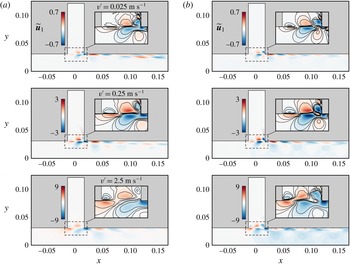
The spatial structure of the harmonic response at $\unicode[STIX]{x1D714}_{1}$ is shown in figure 6, obtained from the LNSE calculation and from the Fourier decomposition (§ 3.1) of LES data. The response is localised in the mixing layer, and in the downstream boundary layer. At low and medium forcing amplitudes, it has a distinct wave packet structure and experiences a clear streamwise growth, with weak perturbations generated close to the upstream corner and amplified while convected by the mean flow to the downstream corner. This is typical of the linear response or instability of mixing layers. At larger forcing amplitudes, the wave packet structure is less well organised and perturbations are convected with no substantial growth. At this frequency, one wavelength of the coherent response (i.e. one vortical structure) almost exactly fills the cavity width. The shape and amplitude of the responses obtained from LNSE and LES are very similar, except in the vicinity of the downstream corner and for the largest forcing amplitudes.

Figure 7.

Contours of streamwise velocity: phase-averaged velocity $\overline{U}+\widetilde{u}_{1}$ and coherent velocity fluctuations $\widetilde{u}_{1}$ . Overlaid are arrows of the phase-averaged and coherent fluctuating velocity fields $\overline{\boldsymbol{U}}+\widetilde{\boldsymbol{u}}_{1}$ and $\widetilde{\boldsymbol{u}}_{1}$ , respectively. (a,b) LES, (c,d) LNSE. Forcing amplitudes: (a,c)  $v^{\prime }=0.025~\text{m}~\text{s}^{-1}$ , (b,d)  $v^{\prime }=2.5~\text{m}~\text{s}^{-1}$ . Time instants in each panel, from top to bottom: $t$ (forcing directed upwards  $\uparrow$ ),  $t+T_{1}/4$ , $t+T_{1}/2$ (forcing directed downwards  $\downarrow$ ) and $t+3T_{1}/4$ .

Figure 8.

Contours of spanwise vorticity: phase-averaged vorticity $\overline{\unicode[STIX]{x1D6FA}}_{z}+\widetilde{\unicode[STIX]{x1D714}}_{z}$ and coherent vorticity fluctuations $\widetilde{\unicode[STIX]{x1D714}}_{z}$ . Overlaid are arrows of the coherent fluctuating velocity field $\widetilde{\boldsymbol{u}}_{1}$ . (a,b) LES, (c,d) LNSE. Forcing amplitudes: (a,c)  $v^{\prime }=0.025~\text{m}~\text{s}^{-1}$ , (b,d)  $v^{\prime }=2.5~\text{m}~\text{s}^{-1}$ . Time instants in each panel, from top to bottom: $t$ (forcing directed upwards  $\uparrow$ ),  $t+T_{1}/4$ , $t+T_{1}/2$ (forcing directed downwards  $\downarrow$ ) and $t+3T_{1}/4$ .

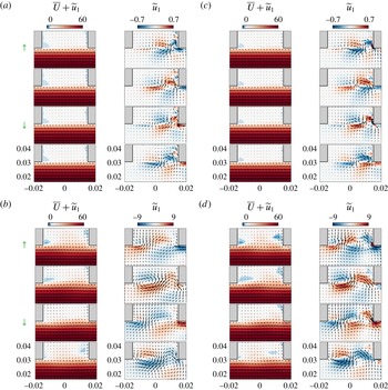
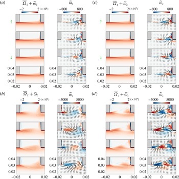
Figures 7 and 8 show snapshots of the response obtained from LES and LNSE at four time instants of an oscillation cycle separated by $T_{1}/4$ , with $T_{1}=2\unicode[STIX]{x03C0}/\unicode[STIX]{x1D714}_{1}$ the forcing period. At small forcing amplitude (figures 7 a,c and 8 a,c), the gain is larger than at other forcing amplitudes but the resulting coherent response is small compared to the mean flow, and oscillations in the total flow are barely distinguishable. Snapshots of streamwise velocity and spanwise vorticity depict the formation and advection of two main vortical structures of opposite vorticity in the first and second half-periods. At larger forcing amplitude (figures 7 b,d and 8 b,d), the amplification is substantially smaller but the coherent response is large enough that fluctuations in the total flow are visible. One can clearly observe the role of the upstream corner in the formation of vortical structures, with $\unicode[STIX]{x1D714}_{z}>0$ when the forcing is directed upwards (towards the cavity end) and, $T_{1}/2$ later, $\unicode[STIX]{x1D714}_{z}<0$ when the forcing is directed downwards (towards the main channel).

As observed in figures 6 and 7, the location of strongest response, where $\widetilde{\boldsymbol{u}}_{1}$ is maximal, moves upstream as the forcing amplitude $|v^{\prime }|$ increases. This is further quantified in figure 9, which represents the streamwise evolution of the coherent kinetic energy integrated vertically in  $J$ ( $y>0$ ), i.e. the coherent energy density

(3.20) $$\begin{eqnarray}E_{y}(x)=\int _{y>0}E(x,y)\,\text{d}y=\frac{1}{2}\int _{y>0}|\widetilde{u}_{1}|^{2}+|\widetilde{v}_{1}|^{2}\,\text{d}y.\end{eqnarray}$$

At low forcing amplitudes, $E_{y}$ increases exponentially with  $x$ , consistent with the streamwise amplification mentioned earlier and with a linear amplification scenario, and reaches its maximum close to the downstream corner. As the forcing amplitude increases, the region of exponential amplification becomes shorter and eventually vanishes; consequently, $E_{y}$ reaches its maximum already near the middle of the cavity, and eventually even in the first half.

Figure 9.

Streamwise evolution of the energy density (3.20). Thick solid lines, LNSE harmonic response; thin dashed lines, LES spectral component.

Figure 10.

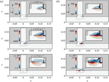
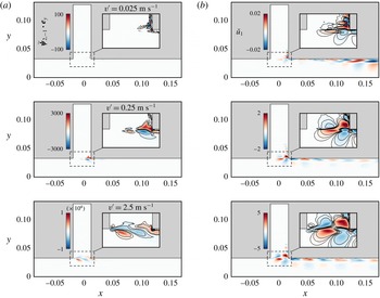
Divergence of the coherent Reynolds stress, $\widetilde{\unicode[STIX]{x1D74D}}_{1,-1}$ (vertical component), acting as a forcing term for the mean flow (see (3.9)). (a) LES. (b) LNSE. Forcing at $\unicode[STIX]{x1D714}_{1}$ , amplitudes $v^{\prime }=0.025$ , 0.25 and $2.5~\text{m}~\text{s}^{-1}$ .

This upstream migration can be understood in terms of the mean flow distortion induced by the Reynolds stresses. As mentioned in § 3, the mean flow is forced by Reynolds stress divergence terms (see e.g. (3.4)). As the forcing amplitude increases, coherent Reynolds stresses build up earlier upstream (figure 10), leading to a thickening of the mean shear layer. In turn, the coherent response building up around this increasingly diffused mean flow benefit from a reduced potential for amplification, and saturate earlier upstream. This segregated yet coupled description, i.e. the interaction between (i) the nonlinear mean flow forced by the coherent response and (ii) the linear monochromatic coherent response around the mean flow, is the central ingredient of the simplified self-consistent model proposed to predict the saturation mechanism at play under harmonic forcing (Mantič-Lugo & Gallaire Reference Mantič-Lugo and Gallaire2016).

4.1 Amplitude of higher harmonics and corresponding forcing terms

In the previous section we have considered the linear response at only one frequency, equal to the forcing frequency $\unicode[STIX]{x1D714}_{1}$ , and we have focused on the external forcing $\widetilde{\boldsymbol{f}}_{1}$ , neglecting other forcing terms arising at $\unicode[STIX]{x1D714}_{1}$ from the interaction of higher-frequency coherent fluctuations, i.e. Reynolds stress divergence terms $\widetilde{\unicode[STIX]{x1D74D}}_{j,1-j}$ ,  $j\geqslant 2$ , in (3.11). The good agreement found between the response obtained in this LNSE framework and the flow computed with a fully nonlinear LES suggests that the nonlinear interaction of higher harmonics plays a negligible role on the response. (Note that this still requires the correct mean flow  $\overline{\boldsymbol{U}}$ , which is crucially determined by $\widetilde{\unicode[STIX]{x1D74D}}_{1,-1}$ and possibly influenced by higher-order terms $\widetilde{\unicode[STIX]{x1D74D}}_{j,-j}$ as well. Here we use the fully nonlinear LES mean flow; a predictive method doing without direct nonlinear simulations would have to account for these Reynolds stresses carefully.) In the following, we investigate this aspect further.

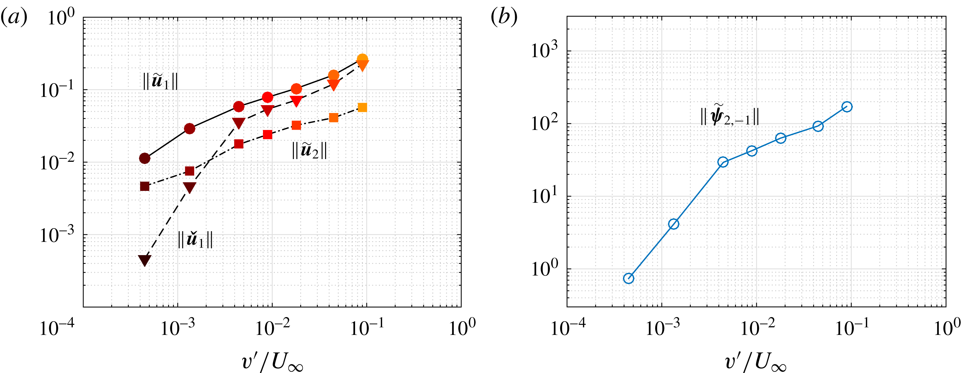
In general, if higher harmonics are small, their interaction is necessarily small too. We note that, in the present flow, the second harmonic $\widetilde{\boldsymbol{u}}_{2}$ (extracted from the LES at $\unicode[STIX]{x1D714}_{2}=2\unicode[STIX]{x1D714}_{1}$ ) is smaller than $\widetilde{\boldsymbol{u}}_{1}$ but far from negligible: the ratio of $L^{2}$ norms $\Vert \widetilde{\boldsymbol{u}}_{1}\Vert /\Vert \widetilde{\boldsymbol{u}}_{2}\Vert$ is less than one order of magnitude (figure 11 a). In Turton et al. (Reference Turton, Tuckerman and Barkley2015), linear stability analysis around the mean flow in a laminar thermosolutal convection system reproduced well nonlinear characteristics for travelling waves whereas it failed for standing waves, which was explained by a negligible (respectively, non-negligible) second harmonic in the former (respectively, latter) case.

Higher harmonics, albeit not negligible, may still contribute only marginally to the harmonic response at $\unicode[STIX]{x1D714}_{1}$ , either (i) if their interaction as Reynolds stress divergence $\widetilde{\unicode[STIX]{x1D74D}}_{j,1-j}$ is small, or (ii) if the response to these forcing terms is small. Regarding condition (i), it would be natural to quantify rigorously what ‘small $\widetilde{\unicode[STIX]{x1D74D}}_{j,1-j}$ ’ means by comparing these forcing terms to the external forcing $\widetilde{\boldsymbol{f}}_{1}$ ; however, this is not possible in the present configuration since the $\widetilde{\unicode[STIX]{x1D74D}}_{j,1-j}$ are defined in the volume while $\widetilde{\boldsymbol{f}}_{1}$ is applied at a boundary. Nonetheless, we report for the sake of completeness the norm of $\widetilde{\unicode[STIX]{x1D74D}}_{2,-1}$ , the first (and likely dominant) Reynolds stress divergence term, in figure 11(b). Regarding condition (ii), which may be verified irrespective of condition (i), comparing the response to each forcing term is straightforward; the question is therefore whether the response to the (possibly non-small) Reynolds stress forcing is small compared to the response $\widetilde{\boldsymbol{u}}_{1}$ to the external forcing:

(4.1) $$\begin{eqnarray}\text{Is}~\Vert \boldsymbol{R}(\unicode[STIX]{x1D714}_{1})\widetilde{\unicode[STIX]{x1D74D}}_{j,1-j}\Vert \ll \Vert \boldsymbol{R}(\unicode[STIX]{x1D714}_{1})\widetilde{\boldsymbol{f}}_{1}\Vert \,?\end{eqnarray}$$

Here we have introduced the resolvent operator $\boldsymbol{R}(\unicode[STIX]{x1D714})=(\text{i}\unicode[STIX]{x1D714}+\boldsymbol{L}(\overline{\boldsymbol{U}}))^{-1}$ . Figure 11(a) reports the norm of $\check{\boldsymbol{u}}_{1}=\boldsymbol{R}(\unicode[STIX]{x1D714}_{1})\widetilde{\unicode[STIX]{x1D74D}}_{2,-1}$ . At the two lowest forcing amplitudes, $\check{\boldsymbol{u}}_{1}$ is indeed much smaller than $\widetilde{\boldsymbol{u}}_{1}$ (in excess of 20 and 5 times, respectively). At larger amplitudes, however, both responses are of the same order of magnitude. At first glance, this seems at odds with the fact that $\widetilde{\boldsymbol{u}}_{1}$ alone is sufficient to predict the overall coherent fluctuations at  $\unicode[STIX]{x1D714}_{1}$ . Interestingly, a closer look reveals that $\check{\boldsymbol{u}}_{1}$ and $\widetilde{\boldsymbol{u}}_{1}$ have different phases and therefore cannot interact constructively, meaning that the norm of the response is essentially unaffected by  $\check{\boldsymbol{u}}_{1}$ .

Figure 11.

(a) Norm of the higher harmonic $\widetilde{\boldsymbol{u}}_{2}$ at $2\unicode[STIX]{x1D714}_{1}$ (LES), of the response $\widetilde{\boldsymbol{u}}_{1}$ to the external forcing $\widetilde{\boldsymbol{f}}_{1}$ at $\unicode[STIX]{x1D714}_{1}$ (LES), and of the response $\check{\boldsymbol{u}}_{1}$ to the first Reynolds stress divergence forcing term $\widetilde{\unicode[STIX]{x1D74D}}_{2,-1}$ at $\unicode[STIX]{x1D714}_{1}$ (LNSE). (b) Norm of $\widetilde{\unicode[STIX]{x1D74D}}_{2,-1}$ .

4.2 Optimal response: harnessing the potential for amplification

Further insight is gained by quantifying how efficiently the two forcing terms (external forcing, and forcing from the interaction of higher harmonics) are amplified. A direct comparison of the gains $\Vert \widetilde{\boldsymbol{u}}_{1}\Vert /\Vert \,\widetilde{\boldsymbol{f}}_{1}\Vert$ and $\Vert \check{\boldsymbol{u}}_{1}\Vert /\Vert \widetilde{\unicode[STIX]{x1D74D}}_{2,-1}\Vert$ gives little information, because the forcing terms are defined on a boundary and in the domain, respectively. However, it is possible to assess whether each forcing efficiently exploits the potential for amplification available in the flow. In this context, it is natural to introduce the concept of optimal gain, which corresponds to the largest possible linear amplification in the flow at a given frequency: instead of solving

(4.2) $$\begin{eqnarray}(\text{i}\unicode[STIX]{x1D714}+\boldsymbol{L}(\overline{\boldsymbol{U}}))\boldsymbol{u}=\boldsymbol{f}\end{eqnarray}$$

to compute the linear response $\boldsymbol{u}$ to a given harmonic forcing $\boldsymbol{f}$ (defined either on a boundary or in the domain), the idea is to identify the optimal forcing $\boldsymbol{f}^{(opt)}$ which maximises the gain

(4.3) $$\begin{eqnarray}G^{(opt)}(\unicode[STIX]{x1D714})=\max _{\boldsymbol{ f}}{\displaystyle \frac{\Vert \boldsymbol{u}\Vert }{\Vert \,\boldsymbol{f}\Vert }}={\displaystyle \frac{\Vert \boldsymbol{u}^{(opt)}\Vert }{\Vert \,\boldsymbol{f}^{(opt)}\Vert }}.\end{eqnarray}$$

With the Euclidean $L^{2}$ norm, the optimal gain is the spectral norm of the resolvent operator  $\boldsymbol{R}$ , which is obtained by performing a singular value decomposition of  $\boldsymbol{R}$ , or, equivalently, by solving the eigenvalue problem $\boldsymbol{R}^{\dagger }\boldsymbol{R}\,\boldsymbol{f}=G^{2}\boldsymbol{f}$ (where $\boldsymbol{R}^{\dagger }$ is the adjoint resolvent operator). If needed, the calculation actually yields more, namely an orthogonal set of optimal forcings $\boldsymbol{f}^{(k)}$ and the corresponding set of optimal responses $\boldsymbol{u}^{(k)}$ associated with optimal gains $G^{(k)}$ sorted in decreasing order:

(4.4) $$\begin{eqnarray}G^{(opt)}=G^{(1)}\geqslant G^{(2)}\geqslant G^{(3)}~\cdots \,.\end{eqnarray}$$

Examples of resolvent analyses around turbulent mean flows include Farrell & Ioannou (Reference Farrell and Ioannou1993), Garnaud et al. (Reference Garnaud, Lesshafft, Schmid and Huerre2013), McKeon, Sharma & Jacobi (Reference McKeon, Sharma and Jacobi2013) and Beneddine et al. (Reference Beneddine, Sipp, Arnault, Dandois and Lesshafft2016).

Figure 12 shows the first three optimal gains for harmonic forcing applied at $\unicode[STIX]{x1D714}_{1}$ at the cavity end or in the domain. At small forcing amplitudes, the first optimal gain is more than one order of magnitude larger than the following optimal gains, which has been observed in other flows (Dergham, Sipp & Robinet Reference Dergham, Sipp and Robinet2013; Boujo & Gallaire Reference Boujo and Gallaire2015; Beneddine et al. Reference Beneddine, Sipp, Arnault, Dandois and Lesshafft2016). At larger amplitudes, this clear separation persists for boundary forcing, while for volume forcing the first optimal forcing becomes increasingly less amplified and is eventually comparable to the following optimal forcings.

Figure 12.

First three optimal gains at $\unicode[STIX]{x1D714}_{1}$ , for (a) boundary forcing at the cavity end $\unicode[STIX]{x1D6E4}_{f}$ , or (b) volume forcing in the domain  $I$ .

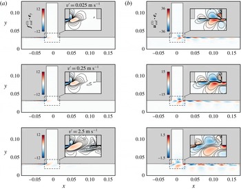
In both cases, the first optimal gain decreases with forcing amplitude, indicating that the dominant amplification mechanism weakens as the mean flow is modified. This is confirmed by the optimal volume forcing and optimal response shown in figure 13: they clearly identify the mixing layer as the main amplification region, and shear as the main amplification mechanism.

Figure 13.

(a) Optimal volume forcing $\boldsymbol{f}_{\!vol}^{(1)}$ at $\unicode[STIX]{x1D714}_{1}$ (unit norm; vertical component). (b) Corresponding optimal response $\boldsymbol{u}_{vol}^{(1)}$ (norm $G_{vol}^{(1)}$ ; streamwise component). Mean flow at forcing amplitudes $v^{\prime }=0.025$ , 0.25 and $2.5~\text{m}~\text{s}^{-1}$ .

The first three optimal boundary forcings at the cavity end $\unicode[STIX]{x1D6E4}_{f}$ are shown in figure 14 for $v^{\prime }=0.075~\text{m}~\text{s}^{-1}$ (they are essentially independent of  $v^{\prime }$ ). They exhibit an increasing number of spatial oscillations over the cavity width. Interestingly, the first optimal is uniform, meaning that the external forcing $\widetilde{\boldsymbol{f}}_{1}$ considered in this study is actually optimal. The response to the optimal boundary forcing has therefore the same structure as the response to $\widetilde{\boldsymbol{f}}_{1}$ shown in figure 6. One can observe that the optimal volume response and optimal boundary response have very similar structures at lower and intermediate forcing amplitudes, i.e. when the first optimal gain is much larger than the following optimal gains.

Figure 14.

First three optimal boundary forcings at the cavity end $\unicode[STIX]{x1D6E4}_{f}$ at $\unicode[STIX]{x1D714}_{1}$ (real part of vertical component of unit-norm $\boldsymbol{f}_{\!bnd}^{(k)}$ ). Mean flow forced at amplitude $v^{\prime }=0.075~\text{m}~\text{s}^{-1}$ .

Figure 15.

Projection coefficients $\unicode[STIX]{x1D6FC}^{(k)}$ on the $k$ th optimal volume forcing $\boldsymbol{f}^{(k)}$ at  $\unicode[STIX]{x1D714}_{1}$ . Coefficients $\unicode[STIX]{x1D6FC}_{bnd}$ and $\unicode[STIX]{x1D6FC}_{vol}$ correspond, respectively, to the external forcing $\widetilde{\boldsymbol{f}}_{1}$ applied at the cavity end, and to the volume Reynolds stress forcing $\widetilde{\unicode[STIX]{x1D74D}}_{2,-1}$ resulting from higher-harmonic interactions.

One might wonder whether the volume forcing term from the Reynolds stress divergence $\widetilde{\unicode[STIX]{x1D74D}}_{2,-1}$ is close to the optimal volume forcing. For a quantitative answer, let us decompose any forcing $\boldsymbol{f}$ (at a boundary or in the domain) using the optimal forcings (  $\boldsymbol{f}_{\!bnd}^{(k)}$ or $\boldsymbol{f}_{\!vol}^{(k)}$ ):

(4.5) $$\begin{eqnarray}\boldsymbol{f}=\mathop{\sum }_{k\geqslant 1}\unicode[STIX]{x1D6FC}^{(k)}\boldsymbol{f}^{(k)}.\end{eqnarray}$$

Since the optimal forcings are orthogonal, the coefficients $\unicode[STIX]{x1D6FC}_{bnd}^{(k)}$ and $\unicode[STIX]{x1D6FC}_{vol}^{(k)}$ are easily expressed in terms of a projection of the considered forcing onto the optimal forcings:

(4.6) $$\begin{eqnarray}\unicode[STIX]{x1D6FC}^{(k)}={\displaystyle \frac{(\,\boldsymbol{f}\mid \,\boldsymbol{f}^{(k)})}{\Vert \,\boldsymbol{f}^{(k)}\Vert ^{2}}}.\end{eqnarray}$$

With this notation, the projection coefficients for the forcing $\widetilde{\boldsymbol{f}}_{1}$ at the cavity end are therefore $\unicode[STIX]{x1D6FC}_{bnd}^{(1)}=1$ , and $\unicode[STIX]{x1D6FC}_{bnd}^{(k)}=0$ for $k\geqslant 1$ . By contrast, the projection coefficients $\unicode[STIX]{x1D6FC}_{vol}^{(1)}$ and $\unicode[STIX]{x1D6FC}_{vol}^{(2)}$ for the forcing arising from higher-harmonic interactions are of the order of $10^{-3}$ – $10^{-2}$ (figure 15), meaning that $\widetilde{\unicode[STIX]{x1D74D}}_{2,-1}$ projects very poorly on the first two optimal volume forcings. In other words, the external forcing $\widetilde{\boldsymbol{f}}_{1}$ harnesses all the amplification available from the cavity end, while $\widetilde{\unicode[STIX]{x1D74D}}_{2,-1}$ only benefits from 0.1–1 % of the amplification available in the domain.

One reason for the poor amplification of $\widetilde{\unicode[STIX]{x1D74D}}_{2,-1}$ is understood by inspecting its spatial structure in figure 16, and that of $\boldsymbol{f}_{\!vol}^{(1)}$ in figure 13. At small and intermediate forcing amplitudes, Reynolds stresses are concentrated in the downstream region of the cavity, while the optimal forcing is localised around the upstream corner. At larger forcing amplitudes, the spatial overlap is better but the projection is still small because the structures remain essentially orthogonal: for instance, $\boldsymbol{f}_{\!vol}^{(1)}\boldsymbol{\cdot }\boldsymbol{e}_{y}$ is uniform over the whole height of the shear layer, while $\widetilde{\unicode[STIX]{x1D74D}}_{2,-1}\boldsymbol{\cdot }\boldsymbol{e}_{y}$ changes sign above and below.

Figure 16.

(a) Reynolds stress divergence $\widetilde{\unicode[STIX]{x1D74D}}_{2,-1}$ (vertical component) forcing the flow at $\unicode[STIX]{x1D714}_{1}$ , from LES. (b) Linear response $\check{\boldsymbol{u}}_{1}$ (streamwise component) to $\widetilde{\unicode[STIX]{x1D74D}}_{2,-1}$ , from LNSE. External forcing at $\unicode[STIX]{x1D714}_{1}$ , amplitudes $v^{\prime }=0.025$ , 0.25 and $2.5~\text{m}~\text{s}^{-1}$ .

5.1 Adjoint-based sensitivity: background

Sensitivity analysis was introduced in the context of hydrodynamic linear stability by Hill (Reference Hill1992), and later used in various parallel (Bottaro, Corbett & Luchini Reference Bottaro, Corbett and Luchini2003), non-parallel 2D (Giannetti & Luchini Reference Giannetti and Luchini2007; Marquet, Sipp & Jacquin Reference Marquet, Sipp and Jacquin2008; Meliga, Sipp & Chomaz Reference Meliga, Sipp and Chomaz2010) and 3D flows (Fani, Camarri & Salvetti Reference Fani, Camarri and Salvetti2012) and in thermoacoustic systems (Magri & Juniper Reference Magri and Juniper2013) to compute the gradient

(5.1) $$\begin{eqnarray}\unicode[STIX]{x1D735}_{\ast }\unicode[STIX]{x1D706}={\displaystyle \frac{\text{d}\unicode[STIX]{x1D706}}{\text{d}\ast }}\end{eqnarray}$$

of an eigenvalue $\unicode[STIX]{x1D706}=\unicode[STIX]{x1D70E}+\text{i}\unicode[STIX]{x1D714}$ with respect to a variety of modifications  $(\ast )$ : (i) steady flow modification, (ii) steady volume/boundary control, and (iii) hypothetical localised ‘velocity-to-force’ feedback (‘structural sensitivity’) (see Chomaz (Reference Chomaz2005) for more details about structural sensitivity, and Luchini & Bottaro (Reference Luchini and Bottaro2014) for a broad review about adjoint equations). The gradient (5.1) is useful information since it immediately predicts, via a simple scalar product, the first-order variation $\unicode[STIX]{x1D706}\rightarrow \unicode[STIX]{x1D706}+\unicode[STIX]{x1D6FF}\unicode[STIX]{x1D706}$ induced by any small-amplitude modification: for instance, a flow modification $\boldsymbol{U}\rightarrow \boldsymbol{U}+\unicode[STIX]{x1D739}\boldsymbol{U}$ induces an eigenvalue variation

(5.2) $$\begin{eqnarray}\unicode[STIX]{x1D6FF}\unicode[STIX]{x1D706}=(\unicode[STIX]{x1D735}_{\boldsymbol{U}}\unicode[STIX]{x1D706}\mid \unicode[STIX]{x1D739}\boldsymbol{U})=\left(\left.{\displaystyle \frac{\text{d}\unicode[STIX]{x1D706}}{\text{d}\boldsymbol{U}}}\right|\unicode[STIX]{x1D739}\boldsymbol{U}\right).\end{eqnarray}$$

For linearly stable flows, Brandt et al. (Reference Brandt, Sipp, Pralits and Marquet2011) extended sensitivity analysis to the linear response to harmonic volume forcing. They found that the sensitivity of the (squared) harmonic gain $G^{2}$ with respect to a modification of the flow $\boldsymbol{U}$ (case (i) above) is given by

(5.3) $$\begin{eqnarray}\unicode[STIX]{x1D735}_{\boldsymbol{U}}G_{vol}^{2}=2G_{vol}^{2}\,\text{Re}\{-\unicode[STIX]{x1D735}\boldsymbol{u}^{\text{H}}\boldsymbol{\cdot }\boldsymbol{f}_{\!vol}+\unicode[STIX]{x1D735}\boldsymbol{f}_{\!vol}\boldsymbol{\cdot }\boldsymbol{u}^{\ast }\},\end{eqnarray}$$

where $\boldsymbol{u}$ is the response to the volume forcing $\boldsymbol{f}_{\!vol}$ , and $(\cdot )^{\text{H}}$ denotes Hermitian transpose (conjugate transpose). Boujo & Gallaire (Reference Boujo and Gallaire2015) considered boundary forcing $\boldsymbol{f}_{\!bnd}$ , in which case the sensitivity of the harmonic gain to flow modification is

(5.4) $$\begin{eqnarray}\unicode[STIX]{x1D735}_{\boldsymbol{U}}G_{bnd}^{2}=2\,\text{Re}\{-\unicode[STIX]{x1D735}\boldsymbol{u}^{\text{H}}\boldsymbol{\cdot }\boldsymbol{u}^{\dagger }+\unicode[STIX]{x1D735}\boldsymbol{u}^{\dagger }\boldsymbol{\cdot }\boldsymbol{u}^{\ast }\},\end{eqnarray}$$

where $\boldsymbol{u}$ is the response to the boundary forcing $\boldsymbol{f}_{\!bnd}$ , and the adjoint perturbation $\boldsymbol{u}^{\dagger }$ is a solution of the adjoint resolvent problem with $\boldsymbol{u}$ as volume forcing (see appendix B for details). From the knowledge of (5.3) or (5.4), one can proceed to compute the sensitivity to control (case (ii) above).

Recently, Qadri & Schmid (Reference Qadri and Schmid2017) proposed an equivalent to structural sensitivity (case (iii) above) for the amplification of harmonic volume forcing. Rearranging their expression, the overall gain variation for a unit feedback localised in $\boldsymbol{x}=\boldsymbol{x}_{0}$ can be recast as

(5.5) $$\begin{eqnarray}\unicode[STIX]{x1D6FF}(G_{vol}^{2})=-2G_{vol}^{2}\,\text{Re}\{\,\boldsymbol{f}_{\!vol}(\boldsymbol{x}_{0})\boldsymbol{\cdot }\boldsymbol{u}(\boldsymbol{x}_{0})\}.\end{eqnarray}$$

When considering boundary forcing, an additional intermediate step is necessary: in this case, the gain variation for a localised unit feedback is

(5.6) $$\begin{eqnarray}\unicode[STIX]{x1D6FF}(G_{bnd}^{2})=-2\,\text{Re}\{\boldsymbol{u}^{\dagger }(\boldsymbol{x}_{0})\boldsymbol{\cdot }\boldsymbol{u}(\boldsymbol{x}_{0})\},\end{eqnarray}$$

where, again, $\boldsymbol{u}^{\dagger }$ is a solution of the adjoint resolvent problem with $\boldsymbol{u}$ as volume forcing (see details in appendix B). A simple way to analyse the sensitivity of the harmonic gain with respect to localised feedback is to look at the space-dependent product

(5.7a,b ) $$\begin{eqnarray}\Vert \,\boldsymbol{f}_{\!vol}(\boldsymbol{x}_{0})\Vert \,\Vert \boldsymbol{u}(\boldsymbol{x}_{0})\Vert \quad \text{or}\quad \Vert \boldsymbol{u}^{\dagger }(\boldsymbol{x}_{0})\Vert \,\Vert \boldsymbol{u}(\boldsymbol{x}_{0})\Vert ,\end{eqnarray}$$

which is analogous to the structural sensitivity of an eigenvalue (product of the direct and adjoint modes).

Figure 17.

Sensitivity of the linear optimal gain $G_{opt}^{2}(\unicode[STIX]{x1D714}_{1})$ , for harmonic forcing at the cavity end  $\unicode[STIX]{x1D6E4}_{f}$ . (a) Magnitude of the sensitivity with respect to mean flow modification (5.4). (b) Structural sensitivity (5.6), i.e. sensitivity with respect to a localised feedback. Forcing amplitudes $v^{\prime }=0.025$ , 0.25 and $2.5~\text{m}~\text{s}^{-1}$ .

5.2 Sensitivity of the optimal gain

In the following we investigate the sensitivity of the optimal harmonic gain for boundary forcing at the cavity end  $\unicode[STIX]{x1D6E4}_{f}$ , at frequency  $\unicode[STIX]{x1D714}_{1}$ . The sensitivity to mean flow modification (5.4) and structural sensitivity (5.6) are shown in figure 17. Both reach their largest magnitude in a localised region near the upstream cavity corner (and, to a lesser extent, in the boundary layer upstream of the cavity as well as in the mixing layer; a second region of large sensitivity appears at the downstream corner as the forcing amplitude $v^{\prime }$ increases). Therefore, the linear amplification between optimal boundary forcing and optimal response is the most sensitive to modifications near the upstream corner.

This is consistent with the fact that most of the amplification is driven by the mean shear: acoustic forcing induces perturbations near the upstream corner, which are then amplified in the mixing layer. Any control aiming at modifying the amplification should therefore target the upstream corner. This also explains why saturation is more marked once fluctuations (Reynolds stresses) have moved upstream, in the region where the mean flow is more sensitive to their effect.

We recall from § 4.2 that (i) the responses to optimal boundary and volume forcing are very similar (in terms of spatial structure), and that (ii) the first optimal gain is almost always much larger than the following optimal gains. These two elements point to a robust amplification mechanism in the mixing layer, fairly insensitive to the exact shape and location of the forcing. In addition, we note that the adjoint perturbation $\boldsymbol{u}^{\dagger }$ in the sensitivities (5.4) and (5.6) looks similar to the optimal response $\boldsymbol{f}^{(opt)}$ , which leads to large sensitivities in exactly the same regions for volume forcing (not shown) and boundary forcing (figure 17).

Figure 18.

Effect of the size of the LNSE domain used to compute the linear response (frequency  $\unicode[STIX]{x1D714}_{1}$ , forcing amplitude $v^{\prime }=0.075~\text{m}~\text{s}^{-1}$ ). (a) Reference domain  $I$ . (b) Smaller domain  $D_{3}^{xy}$ .

Finally, we observe that the linear gain does not vary substantially when reducing the size of the computational domain, as long as the boundaries are not too close to the region of large structural sensitivity (see details in appendix C). The spatial structure of the response is unaffected too (figure 18). This is in agreement with Giannetti & Luchini (Reference Giannetti and Luchini2007), who found a similar behaviour for the leading eigenvalue and eigenmode of the flow past a circular cylinder at $Re=50$ : they hypothesised that ‘the characteristics of the global mode are dictated mainly by the conditions existing in the region where values of [structural sensitivity] substantially different from zero are attained’, i.e. where the global mode and associated adjoint mode overlap. We formulate the same hypothesis in the case of harmonic amplification: the value of the linear gain and the spatial structure of the response are dictated mainly by the flow in the region where structural sensitivity is not small, i.e. where the response $\boldsymbol{u}$ and the volume forcing $\boldsymbol{f}$ (or the adjoint perturbation $\boldsymbol{u}^{\dagger }$ associated with boundary forcing) overlap.