I. INTRODUCTION
Low-dimensional nanomaterials such as carbon nanotubes (CNTs),Reference Iijima1, Reference Dai2 nanowires,Reference Duan and Lieber3, Reference Wu, Xiang, Yang, Lu and Lieber4 and grapheneReference Geim and Novoselov5 have properties that are very different from bulk materials. Although these properties are usually attributed to their high surface area to volume ratio or quantum confinement effects, these materials are distinct from the bulk in another important way. Low-dimensional nanostructures can be flexible and may not be straight/flat at equilibrium. These shapes arise because of a compromise between bending energy and other forces, for example, surface stress, internal stress, electrostatic interaction, or adsorption. There are myriad examples of such nanostructures, including ZnO and SnO2 nanobelts,Reference Kong and Wang6, Reference Pan, Dai and Wang7 graphene nanoribbons (GNRs),Reference Bets and Yakobson8 silica/carbonate helicoids,Reference Garcia-Ruiz, Melero-Garcia and Hyde9 SiGe nanodrills,Reference Huang, Boone, Roberts, Savage, Lagally, Shaji, Qin, Blick, Nairn and Liu10 and SiGe/Si/Cr nanocoils.Reference Zhang, Deckhardt, Weber, Schonenberger and Grutzmacher11
Because thermodynamic properties are defined relative to an equilibrium state, the properties of a nanostructure will depend on the shape of that structure. Although these shapes are not unique to the nanometer scale, they are more common in nanostructures because of the strong influence of surfaces and low mechanical rigidity. This observation leads us to classify nanostructures based on the number of dimensions into which they can spontaneously deform c. Formally, c is the codimension of the nanostructure: the difference between the dimensionality of the space in which the material is embedded D (i.e., in which it can deform), and the intrinsic dimensionality of the object d.Reference Hazewinkel12, 13 The codimension is a measure of the spatial degrees of freedom of the nanostructure. For example, a graphene sheet and a nanowire embedded in a three-dimensional space has codimension c = 3 − 2 = 1 and c = 3 − 1 = 2, respectively. If a nanowire, in three dimensions, is constrained to remain straight (i.e., it is prevented from deforming into the other two dimensions), it has codimension c = 1 − 1 = 0.
The properties of a nanostructure can be distinct from the properties of the corresponding bulk material. The thermodynamic properties of a nanostructure are defined relative to nanoscale variables. For example, for a nanowire, we may be interested in the application of a mechanical load along its axis. Two relevant thermodynamic variables are the length of the nanowire and the force on the ends of the nanowire. Obviously, if a flexible nanostructure bends rather than stretches, it will appear to have a very small stiffness. In other words, the thermodynamic properties of the nanostructure depend on how the material deforms. In contrast, bulk thermodynamic quantities, such as the Young’s modulus, are defined relative to the microscopic strain state of a volume element.
This study examines how a flexible, low-dimensional nanostructure with c = D − d > 0 can have very different properties than the same material in c = 0. In c = 0, structures will be “bulklike,” whereas in c > 0, their shape may be important. We further propose that for low-dimensional, flexible objects, these c-dependent properties may be engineered by introducing interactions with a stiff substrate. In the following sections, we discuss three examples of how codimension affects properties. We first illustrate this idea using a “toy” model for thermal expansion of a flexible material. Then, we discuss the c dependence of the stiffness of nanowires and the edge energy and edge stress of GNRs.
II. THERMAL EXPANSION OF A BEAD CHAIN IN c ≥ 0
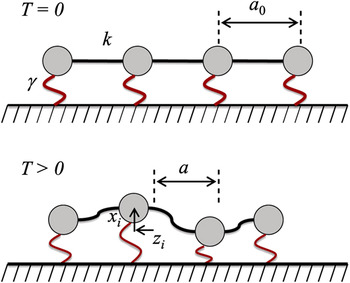
In order to illustrate the generic relationship between codimension and materials properties, we consider a model system of a chain of N beads connected by linear springs of stiffness k and equilibrium length a 0 at T = 0. The position of the ith bead is described by ri. This geometry is illustrated in Fig. 1. At any finite temperature, a bead chain will tend to crumple into a compact (rather than linear) configuration because of its lack of bending rigidity. To prevent crumpling, the chain can be placed in a strong external potential  , where γ is the interaction strength and x i is the displacement of the ith bead perpendicular to the nominal chain axis. This potential penalizes deformations out of the chain-line direction (z in this example, Fig. 1). We analyze this model for cases where beads can move in different codimensions, and we find that the sign of the coefficient of thermal expansion (CTE) is determined by the codimension of the space.
A modified bead-chain model is illustrated at T = 0 and at T > 0. The beads are connected to each other by springs with harmonic constant k and are connected to the substrate with springs with harmonic constant γ. Here, a 0, the equilibrium lattice constant at T = 0, is in general different from a, the average lattice spacing at T > 0. The position of the ith atom is described relative to a crystalline lattice using the displacements xi and zi.

In D = 2 (c = 1), the potential energy of this system is written as

where ri = (xi, zi + ia) and a is the lattice constant of the system at the temperature of interest. We consider this model in the limit that the vibrations of the beads are small compared to a. In this limit ( , for all i), we may linearize U as
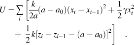
We calculate a rigorous upper bound for the Helmholtz free energy A(T, L) using the Gibbs–Bogoliubov inequality,

where the free energy and potential energy of a reference state are A 0 and U 0, respectively. Following the methods of LeSar et al.Reference LeSar, Najafabadi and Srolovitz14 and Mansoori et al.,Reference Mansoori and Canfield15 we perform a variational calculation, choosing the reference state to be an Einstein solid with lattice parameter a. In this case, the probability of finding a bead displacement (xi, zi) is described by a Gaussian function centered around a lattice site,  , where αx and αz are constants. The A 0 for this Einstein solid is

where Γ is the thermal wavelength and N is the number of beads. The expression 〈U〉0 is found by averaging U over the Gaussian functions,

where Δ = (a − a 0)/a. According to the equipartition theorem, 〈U 0〉0 = Nk BT. We can approximate A by optimizing A 0 +〈U − U 0〉0 with respect to a. Next, we determine the CTE in arbitrary codimension c = D − 1 by taking the appropriate derivative of the free energy:
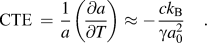
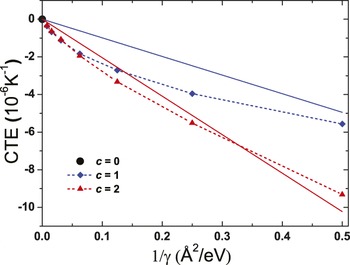
In order to test this result, we perform molecular dynamics on this modified bead-chain model. The molecular dynamics simulation was initialized by arranging all of the beads in a linear chain, with lattice spacing a 0 = 3 Å. The system is equilibrated at low temperatures using a NVT thermostat, and the lattice constant (mean spacing between beads) is measured as a function of the temperature. The results are presented in Fig. 2.
CTE of a nominally linear chain of beads connected by harmonic springs as a function of the inverse confinement interaction strength 1/γ in codimensions c = 0, 1, and 2. Continuous solid lines show the analytical result and dotted lines connect molecular dynamics data points.

Figure 2 shows that the CTE → 0 as γ → ∞. This is because this model is purely harmonic. Very large values of γ imply that the chain is constrained to be linear, and so the effective codimension is c eff ≈ 0. Smaller values of γ imply more freedom to explore higher dimensions (i.e., weaker confinement) and greater deviations from c = 0. Here γ can be interpreted as a measure of mechanical constraint that continuously interpolates between c = 0 and the maximum codimension c > 0. Equation (6) is derived assuming strong confinement, in which γ > 0 (i.e., nearly straight). However, we note that at any finite temperature if a straight bead chain is under no confinement (not describable based on the perturbative approach of Eq. (6), then an entropic force will tend to bring the two ends together. If we take the reference state to be the fully extended chain at T = 0, the chain will always have a negative CTE.
Our bead-chain model qualitatively describes the behavior of nearly linear polymer chains, such as the polymer chains within CNTs that have recently been observed.Reference Steinmetz, Kwon, Lee, Abou-Hamad, Almairac, Goze-Bac, Kim and Park16–Reference Bazilevsky, Sun, Yarin and Megaridis19 A polymer chain inside a very narrow CNT corresponds to c eff = 0, because the confinement would constrain the polymer chain, severely restricting its displacements away from the CNT axis. McIntosh et al.Reference McIntosh, Tománek and Park20 calculated the equilibrium distance between a polyacetylene chain and a CNT wall to be 3.3 Å. Based on their estimates a (4,4) and (5,5) arm chair CNT would provide strong confinement and have therefore c eff ≈ 0. In contrast for, wide CNTs, the confinement would the reduced, leading to c eff > 0; for example, a (6,6), (7,7), or wider CNT is predicted to provide much less confinement and have therefore c eff > 0. Other approachs to modify the c eff of a polymer within a nanotube include stiffening the nanotube by going from single to multiwall tubes, increasing the diameter of the polymer chain by modification of the polymer side groups, and varying the number of polymer chains inside the CNT.
It is useful to compare our predictions to predictions for related systems. The present findings are consistent with the predicted low temperature behavior of graphene. Although the CTE of graphene is positive in c = 0 (i.e., the material is not perfectly harmonic), recent experiments show that the CTE of graphene in c = 1 is negative at low temperature and becomes positive at higher temperature.Reference Bao, Miao, Chen, Zhang, Jang, Dames and Lau21 This is consistent with our bead-chain results above and the calculations of Jiang et al.Reference Jiang, Wang and Li22 However, if a strong substrate interaction is imposed (c eff ≈ 0), the CTE becomes positive at all temperatures.Reference Jiang, Wang and Li22 Using the example of CTE, we have shown that properties can be tuned by appropriately changing the codimension. In the next section, we discuss the implications of codimension on other classes of properties.
III. THE STIFFNESS OF A NANOWIRE IN c ≥ 0
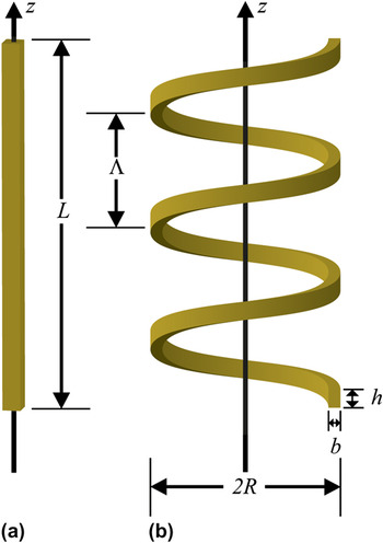
Another clear example of the effects of codimension on materials properties may be found in the dependence of the elastic response of a nanowire on its equilibrium shape. Consider the case of nanowires that, in equilibrium, exhibit a helical or springlike shape (i.e., nanohelices) as, for example, recent observations in ZnO,6 SiC,Reference Zhang, Alkhateeb, Han, Mahmood, McIlroy and Norton23 and SiGe/Si/Cr.Reference Zhang, Deckhardt, Weber, Schonenberger and Grutzmacher11 Because the nanohelix deforms in three dimensions upon application of a tensile load, it is a c = 3 − 1 = 2 structure; in contrast, a straight nanowire deforms in one dimension (i.e., c = 1 − 1 = 0). The stiffnesses of these two structures will be very different. In this section, we explicitly compare the elastic response of two nanowires, in a helical and straight (rod) form, with the same cross-sectional dimensions and same end-to-end distance L. Of course, a much greater force is required to stretch a straight nanorod to the same extent as a nanohelix.
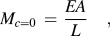
The stiffness of a straight wire with end-to-end distance L and uniform cross section [see Fig. 3(a)] is calculated using Hooke’s law,
(a) Schematic illustrations of a straight rod (c = 0) with a rectangular cross section and (b) a similar rod in an equilibrium helical spring configuration (c = 2). The relevant geometrical parameters defining the helical spring are the cross-section width (h) and thickness (b), the mean coil radius R, and the helix pitch Λ.

where E is the Young’s modulus of the material and A is the cross-sectional area of the rod. In contrast, if the wire is a helix, its stiffness can be calculated using standard mechanics methods,Reference Wahl24–Reference Young and Budynas26
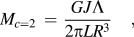
where L is the end-to-end length of the helix, R is the radius of the coil, Λ is the helix pitch, J is the torsion constant, and G is the shear modulus of the material, as illustrated in Fig. 3(b). If one bends a wire into a helix, it will have a shorter end-to-end length than the length L of the wire. The stiffness of this object can be calculated from Eq. (8) by scaling L by the geometrical factor Λ/2πR.
Comparing Eq. (7) and Eq. (8), we find that the spring constant of a helix relative to that of a rod with the same end-to-end length is reduced by a factor
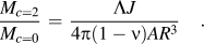
Using Eq. (9), we can predict the magnitude of the reduction in the spring constant of the ZnO nanohelices produced by Kong and WangReference Kong and Wang6 relative to straight ZnO nanoribbons of the same length and cross section. For this case, the spring constant ratio is
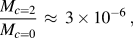
where we have substituted the geometical parameters from the Kong and WongReference Kong and Wang6 results (typical radii of R = 500 nm, pitch of Λ = 150 nm, and rectangular cross sections of h × b = 30 × 10 nm) and the torsion constant from Young and Budynas.Reference Young and Budynas26 Note that there is an approximately 1 million times reduction in the force required to stretch a c = 2 nanohelix as compared with stretching a c = 0 straight nanorod to the same extension.
IV. THE EDGE ENERGY AND STRESS OF A GNR
Graphene is a nominally two-dimensional, flexible, model nanomaterial. It has attracted considerable theoretical and experimental attention since graphene sheets and GNRs were first fabricated.Reference Geim and Novoselov5, Reference Gass, Bangert, Bleloch, Wang, Nair and Geim27–Reference Geim29 In this section, we use codimension to reinterpret two important materials properties of graphene: the edge energy and the edge stress.
Recent theoretical studies found that graphene edges can exhibit large compressive edge stresses.Reference Jun30–Reference Gan and Srolovitz32 Empirical potential calculations have shown that in c = D − d = 3 − 2 = 1, this compressive stress can cause edge warping or GNR twisting,Reference Bets and Yakobson8, Reference Shenoy, Reddy, Ramasubramaniam and Zhang33 in qualitative agreement with the elastic behavior of macroscopic plates.Reference Rammerstorfer, Fischer and Friedl34 Experiments have also shown that graphene and boron nitride nanoribbons can extensively bend and twist and have their edges rippled to accommodate the stress.Reference Chen, Zou, Liu, Li, Wang, Wang, Yuan, Sekiguchi, Cheng and Lu35, Reference Campos-Delgado, Romo-Herrera, Jia, Cullen, Muramatsu, Kim, Hayashi, Ren, Smith, Okuno, Ohba, Kanoh, Kaneko, Endo, Terrones, Dresselhaus and Terrones36
The edge energy is given by

where we have defined the edge stress τ e as the energy cost required to deform a GNR edge by an infinitesimal strain ɛ parallel to the edge from the equilibrium configuration at ɛ = 0.
In differential form,
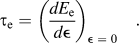
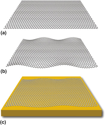
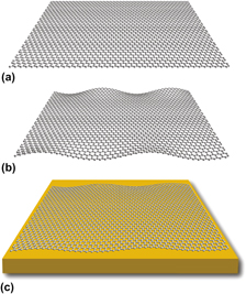
Figure 4(a) shows a GNR that is constrained to c = 0 by restricting the sheet to D = 2. We determine the properties of this GNR and of several other GNRs for edge orientations between (and including) the well-studied armchair and zigzag orientations.Reference Branicio, Gan, Jhon and Srolovitz37 As indicated in Fig. 5(a) (atoms in local armchair/zigzag edge configurations are shown in orange/red), intermediate orientations contain segments of both the armchair and zigzag edge geometries.
GNRs illustrated in different codimensions c. (a) A flat GNR (c = 0) at T = 0. (b) The same GNR as in (a) that spontaneously deforms into a third dimension (c = 1). In this case, the compressive edge stresses lead to edge warping while the interior of the GNR remains flat. (c) A GNR interacting with a substrate resulting in an effective codimension c between (a) c = 0 and (b) c = 1. For this case the warping will have a lower magnitude than for (b).

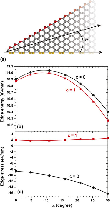
Edge energies and stresses for arbitrary graphene edges. (a) The definition of the edge angle α with respect to a graphene sheet; α = 0° corresponds to the armchair edge (yellow) and α = 30° to the zigzag edge (red). (b) Graphene edge energy E e as a function of edge angle 0° < α < 30°. Values are shown for c = 0 and 1. (c) Graphene edge stress τ e for the same edges as in (b).

We determine the equilibrium GNR structure at T = 0 by minimizing the total energy with respect to all atom coordinates using the reactive empirical bond order potential (REBO-II)Reference Brenner, Shenderova, Harrison, Stuart, Ni and Sinnott38 and imposing periodic boundary conditions along the GNR length. The edge energy E e, determined in this equilibrium configuration, is shown in Fig. 5(b). The edge stress τ e for the relaxed GNRs is shown in Fig. 5(c) and is obtained from the slope of a plot of edge energy E e versus uniaxial strain (parallel to the ribbon axis). Details of the calculation of edge energy and stress can be found in Appendix A. Both E e and τ e for the relaxed GNRs vary smoothly with orientation α, and E e varies by less than 10% with edge angle α. In contrast, the variation of the edge stress τe with α is much larger (∼50%). The magnitude of both quantities is in reasonable agreement with density functional theoryReference Jun30–Reference Gan and Srolovitz32, Reference Liu, Dobrinsky and Yakobson39 and empirical potential calculations.Reference Shenoy, Reddy, Ramasubramaniam and Zhang33, Reference Liu, Dobrinsky and Yakobson39, Reference Lu and Huang40 The results shown in Fig. 5(b) closely follow the analytical expressions for the edge energy reported recently.Reference Branicio, Gan, Jhon and Srolovitz37, Reference Liu, Dobrinsky and Yakobson39
When a GNR is embedded in three dimensions (D = 3) rather than two (i.e., the GNR is not constrained to be flat), the edges buckle in the direction normal to the GNR plane, producing the edge ripples seen in Fig. 4(b). The rippling or warping decays away from the edge toward the interior of the GNR, which remains nearly flat, in agreement with earlier simulations.Reference Shenoy, Reddy, Ramasubramaniam and Zhang33
The effect of codimension on GNR edge properties is illustrated in Fig. 5. The edge energy E e changes very little with codimension. In contrast, the edge stress τ e changes sign (goes from strongly compressive to slightly tensile) upon increasing the codimension from c = 0 to c = 1 (i.e., allowing relaxation into the orthogonal direction). These results show that although some properties (e.g., τ e) change dramatically with codimension, other related properties (e.g., E e) are nearly independent of c.
These results raise some questions. What edge stress would be measured in an experiment? Would it be the large c = 0 compressive stress or would it be the relaxed, tensile stress for c = 1? If a free-standing GNR of a length that is large compared to the edge rippling wavelength is stretched along its axis, clearly the edge stress would be τ c=1 not τ c=0. In contrast, if a GNR is strongly bonded to a substrate and the system is stretched in the same manner, the edge stress would be τ c=0 not τ c=1.
Intuitively, we can imagine that by applying a mechanical constraint to the graphene sheet, we can engineer the edge stress. A natural way to do this is to adsorb graphene onto a substrate. A recent experimental study by Lui et al.Reference Lui, Liu, Mak, Flynn and Heinz41 in which graphene was deposited on flat mica surfaces showed that the resultant graphene sheets were ultraflat compared with free or suspended graphene. By controlling the chemical nature of the surface it would be possible to modify the degree of constraint that would accompany that adsorption of graphene. For example, free standing graphene would correspond to c = 1, graphene on a gold substrate to c = 0, but graphene on a gold substate on which thiols were chemisorbed prior to graphene adsorption would lead to a relatively weak constraint of the graphene, yielding an effective codimension 0 < c eff < 1 [see Fig. 4(c)].
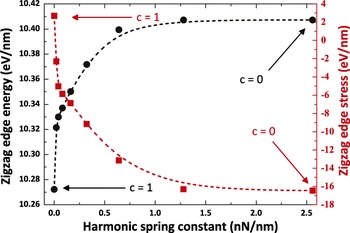
We investigate this possibility by modeling the interaction of graphene with a substrate and its effect on edge properties by introducing a harmonic potential  that penalizes out-of-plane deformation. We then recalculate the edge stress as a function of γ. As shown in Fig. 6, the edge stress τ e varies rapidly with the strength of the bonding to the substrate, but the edge energies E e show only a very weak dependence on the strength of the bonding γ. This reinforces our earlier conclusions on the effect of codimension on GNR edge properties.
Codimension dependence of graphene zigzag edge energy E e and edge stress τ e. The effective codimension varies from c eff = 0 to c eff = 1 by changing the strength of the harmonic interaction γ with a rigid substrate. Although these results are for the zigzag edge, similar dependences are found for the other edge orientations.

V. DISCUSSION
We have demonstrated, through a disparate series of examples, that low-dimensional materials have properties that can be strongly dependent on the dimensionality of the space in which they “live.” This peculiar condition is captured by the broad codimension concept. This can be related to two other very important, general principles. First, codimension is quite similar to the degree of freedom concept. The codimension dictates the geometrical degrees of freedom that a low dimensional material can access. However, these degrees of freedom are not arbitrary, but are instead determined by the flexibility of the structure. Second, codimension is a generalization of the concept of mechanical constraint. Constraint is typically only applied to mechanical properties, but we have shown that it can be applied more broadly, such as to thermal expansion.
This discussion allows us to speculate on the types of properties that are likely to be highly c-dependent. Because of the increased degrees of geometric freedom, bending and twisting in nanostructures breaks the local crystal symmetry. This changes the symmetry constraints on equilibrium properties and can make such properties sensitive to codimension changes. Consider the spontaneous polarization of a ferroelectric nanohelix, such as ZnO. Even if the dipole moment of each unit cell does not change on going from the bulk to a nanowire geometry, the spontaneous polarization will change dramatically with the radius and pitch of the equilibrium helical structure. Similarly, the piezoelectric constants of a nanohelix will be much reduced compared with when the same material is a straight nanorod. In general, deformation into higher dimensions will have a small effect on properties that are determined largely by point group symmetry, because the magnitude of equilibrium deformations is usually small. By contrast, bending and twisting in a higher codimension can have a large effect on space group-dependent properties, for example, introducing a screw axis (as in a helix) modifies at least one translational symmetry. The effect of crystal symmetry on anisotropic material properties can be pronounced, as described in detail by Nye.Reference Nye42 A classical example is that of birefringence, where symmetry breaking due to mechanical deformation can cause an isotropic material to show an anisotropic materials property. Using the terminology of Nye, coupled effects to deformation will be particularly affected. In thermoelastic systems, these properties include the heat of deformation, thermal expansion, piezocaloric effects, and thermal pressure. When other fields are considered, further properties include piezoelectricity and magnetostriction.
Codimension can also be used to understand more sophisticated nanostructure shapes that have a fractal character. Nanostructures such as polymer, nanotube, or nanowire networks can have a fractal dimension and therefore a noninteger codimension c < 2. We can contrast the properties of these fractal structures to those of linear, c = 2 structures. Such fractal nanostructures have, as a fundamental structural unit, point defects or branch/bifurcation points.Reference Ovid’ko43 Examples of simple nanostructures containing such defects are X-, Y-, and T-shaped CNT junctions, which have recently been observed.Reference Terrones, Banhart, Grobert, Charlier, Terrones and Ajayan44 Composites reinforced with Y junctions have dramatically different strengths and toughnesses compared to those with straight nanotubes.Reference Gutkin and Ovid’ko45, Reference Gutkin and Ovid’ko46 This suggests that the properties of fractal structures will be similarly affected compared to linear materials.
Although the concept of codimension-dependent properties was discussed in the context of nanostructures, it is general and applies to all low-dimensional systems that exhibit equilibrium shapes that are deformed relative to the common c = 0 case (i.e., c > 0). Two such examples are hippuric acid needlesReference Shtukenberg, Freudenthal and Kahr47 and long leaves,Reference Liang and Mahadevan48 which respectively twist and bend during growth. Their properties should change similarly to our previously discussed examples. As a final note, we initially defined codimension as a fixed and integer value. As shown in the discussed examples, the effective codimension c eff need not necessarily be an integer. In principle, it can be made to vary continually between two values. Properties can than be engineered by adjusting the values of the effective codimension.
VI. CONCLUSIONS
When materials are very thin in one or more dimensions, their equilibrium shape is often deformed (relative to the bulk material). This can be the result of, for example, surface stress, internal stress, piezoelectricity, and electrostatics. Because material properties are variations of appropriate thermodynamic potentials from the equilibrium state, such equilibrium deformation may modify many material properties. Although these changes are profound for some properties, such as edge stress in graphene and the stiffness of a nanohelix, they have little effect on others, such as edge energy in graphene. For those properties that are sensitive to equilibrium deformation, their magnitude will be sensitive to the number of degrees of freedom that are accessed during deformation, that is, the codimension. This suggests new approaches to engineer nanomaterial properties.
ACKNOWLEDGMENTS
The authors gratefully acknowledge Prof. M. Haataja, Prof. Y.W. Zhang, Prof. S. Safran, Prof. C. Arnold, Dr. C.K. Gan, and Dr. C. Majidi for enlightening discussions and comments.
APPENDIX A: CALCULATION OF GRAPHENE EDGE ENERGY AND STRESS
GNR edge energy and stress are calculated in a similar manner as JunReference Jun30 and Gan and Srolovitz.Reference Gan and Srolovitz32 The edge energy (per unit length) E e as a function of edge orientation α is defined as

where  is the total energy of a GNR with N atoms, length L, and edge orientation α, and E B is the energy per atom in a bulk (infinite) flat graphene sheet. The factor of 2 in the denominator of Eq. (A1) accounts for the fact that a GNR has two (parallel) edges. For narrow GNRs, E e(α) depends on the GNR width because of interactions between the edges. This effect decays rapidly with GNR width. Therefore, we perform simulations on GNRs of widths in excess of 100 Å for which E e(α) reaches the asymptotic value for large widths.
For all edge types, E e(α) was calculated by minimizing the total energy with respect to all atomic coordinates at T = 0. We employed the limited-memory Broyden–Fletcher–Goldfarb–ShannoReference Liu and Nocedal49 method to relax the atomic structures (both in c = 0 and 1) until it converged to within 10−10 eV/atom. In the c = 1 case, noise was added to the initial atomic positions (i.e., perturbations in the atom positions from the flat structure) in order to break the symmetry of the problem.
We calculate the edge stress τ e by straining the equilibrium (zero stress) GNR and interpolating the resultant system energy versus strain curve at ɛ = 0. For c = 0, both compressive and tensile strains were employed, for c = 1, where the GNR buckles out of plane for compressive strains, only tensile strains were applied in order to determine τ e.