1. Introduction
People have always dreamed of flying like birds. But just over a century ago, in the works of Kutta, Joukowski and Chaplygin (plane theory) and also Lanchester and Prandtl (lifting-line theory), the foundation of the mathematical theory was laid for determining the aerodynamic characteristics of a wing in a steady gliding flight (with fixed wings). The mathematical theory of a flapping flight began to develop at about the same time. Prandtl (Reference Prandtl1924) formulated the problem of unsteady wing motion, which in the linear approximation was solved in the work of Birnbaum (Reference Birnbaum1924). The solution gave qualitative estimates of the thrust force generated by the wing. The Prandtl–Birnbaum approach, based on the introduction of vortex sheets inside an ideal fluid, was further developed by Wagner (Reference Wagner1925), Glauert (Reference Glauert1930), Keldysh & Lavrentiev (Reference Keldysh and Lavrentiev1935), Theodorsen (Reference Theodorsen1935), Nekrasov (Reference Nekrasov1947), Sedov (Reference Sedov1966) and Giesing (Reference Giesing1968). Theodorsen (Reference Theodorsen1935) formulated a theory for the calculation of the hydrodynamic forces acting on the airfoil in the case of low-amplitude harmonic oscillations, assuming that the wake of the airfoil would take the form of a continuous vortex sheet of varying strength. Garrick (Reference Garrick1936) further developed the theory of Theodorsen and obtained an expression for the thrust force acting on an oscillating flat plate. von Kármán & Burgers (Reference von Kármán and Burgers1935) described the special structure of the vortex wake behind an oscillating airfoil. It turned out to be similar to the classical Kármán vortex street, but with the opposite direction of rotation of the vortices (also called the Golubev vortex street). Such vortices are involved in the transfer of momentum in the direction opposite to the motion of the airfoil; this is the cause or consequence of the formation of the thrust force. The research approach based on such a flow model was developed by Golubev (Reference Golubev1949, Reference Golubev1951).
In the 1960–1980s, a new direction of research began to develop associated with the propulsive motion of a dynamically deformable body. One of the first works in this direction belongs to Lighthill (Reference Lighthill1960), who studied the thrust created by the undulating motion of a long cylindrical body of a variable cross-section in an inviscid fluid. Subsequently, the analytical theory of the propulsive motion of a dynamically deformable body was developed in the works of Lavrentyev & Lavrentyev (Reference Lavrentyev and Lavrentyev1962), Lighthill (Reference Lighthill1970), Logvinovich (Reference Logvinovich1970), Wu (Reference Wu1971) and Newman & Wu (Reference Newman and Wu1975).
Since the late 1980s, the focus of research has shifted from analytical modelling to the numerical simulations of the aerohydrodynamics of a flapping flight and swimming. Nowadays, a significant number of studies of bird and fish motion based on two-dimensional and three-dimensional numerical models has been carried out (e.g. Liu et al. Reference Liu, Ellington, Kawachi, van den Berg and Willmott1998; Isogai, Shinmoto & Watanabe Reference Isogai, Shinmoto and Watanabe1999; Lewin & Haj-Hariri Reference Lewin and Haj-Hariri2003; Pedro, Suleman & Djilali Reference Pedro, Suleman and Djilali2003; Alben & Shelley Reference Alben and Shelley2005; Spagnolie et al. Reference Spagnolie, Moret, Shelley and Zhang2010; Zhang, Liu & Lu Reference Zhang, Liu and Lu2010; Maertens, Triantafyllou & Yue Reference Maertens, Triantafyllou and Yue2015; Lua et al. Reference Lua, Dash, Lim and Yeo2016; Taha Reference Taha2020; Alben Reference Alben2021a,Reference Albenb). A detailed review of the development of all of the above models to date can be found in the works of Rozhdestvensky & Ryzhov (Reference Rozhdestvensky and Ryzhov2003) and Wu et al. (Reference Wu, Zhang, Tian, Li and Lu2020).
Despite the success of numerical modelling, questions about the key principles of flapping flight and about the hydrodynamic mechanisms of creation of thrust by a flapping wing can be fully discovered only within the framework of analytical theory. The basis of most of the analytical studies of a flapping wing (as shown above) is the model of an ideal fluid, supplemented by special assumptions about the nature of flow separation (e.g. Birnbaum Reference Birnbaum1924; Prandtl Reference Prandtl1924; Theodorsen Reference Theodorsen1935; Sedov Reference Sedov1966), the structure of the vortex wake (e.g. Golubev Reference Golubev1949, Reference Golubev1951), etc. In this study, we develop a different approach based on the method of asymptotic expansions of the solution of the complete system of Navier–Stokes equations in the small parameter (e.g. Schlichting Reference Schlichting1932; Holtsmark et al. Reference Holtsmark, Johnsen, Sikkeland and Skavlem1954; Riley Reference Riley1967, Reference Riley1975; Wang Reference Wang1968; Riley & Watson Reference Riley and Watson1993; Nuriev & Egorov Reference Nuriev and Egorov2019; Nuriev, Egorov & Kamalutdinov Reference Nuriev, Egorov and Kamalutdinov2021), which is used to solve the problem of rotational–translational oscillations of a cylinder in a flow. As a small parameter, the ratio of the amplitude  $A$ of transverse oscillations to the radius
 $a$ of the cylinder,
 $\gamma = A/a$, is taken.
Solution for the case of purely translational oscillations of a circular cylinder in the main term  $O(\gamma ^0)$ was first obtained by Stokes (Reference Stokes1851). In the second approximation, this problem was first solved by Holtsmark et al. (Reference Holtsmark, Johnsen, Sikkeland and Skavlem1954). The term
 $O(\gamma ^1)$ contains a stationary component that describes the so-called steady streaming (this effect was first described by Schlichting (Reference Schlichting1932) from a theoretical point of view). For the case of low-amplitude transverse harmonic oscillations of a circular cylinder (e.g. Holtsmark et al. Reference Holtsmark, Johnsen, Sikkeland and Skavlem1954; Egorov & Nuriev Reference Egorov and Nuriev2021), such flows are symmetric, decay at infinity and do not cause steady hydrodynamic forces (thrust or lift).
An asymptotic study of the problem of rotational–translational oscillations of a circular cylinder was first carried out by Riley & Watson (Reference Riley and Watson1993). The work mainly considered the structural features of secondary streaming under conditions of zero average speed of motion. For the case of high frequencies, the authors noted the appearance of a non-zero average force acting on the cylinder. However, to date, this line of research has not received further development. The formation of a stationary force component during rotational–translational oscillations of a circular cylinder in the framework of a numerical study was described by Blackburn, Elston & Sheridan (Reference Blackburn, Elston and Sheridan1999). The authors have shown that under the influence of this force, the body can switch to a directional regime of motion with a cruising speed of 33 % of the peak speed of oscillations (the results of calculations are presented in the work only for one case). Also, the possibility of propulsive motion of an oscillating circular cylinder was considered in a numerical study of Koehler et al. (Reference Koehler, Beran, Vanella and Balaras2015). The authors studied streaming jet regimes formed during rotational–translational oscillations of a cylinder in a quiescent fluid, in particular, the possibility of varying the deflection angles of jets and, accordingly, redirecting the thrust vector.
In this work, we will show that the development of the asymptotic approach gives ample opportunity to study the propulsive motion of a cylinder performing rotational–translational oscillations. In contrast to Riley & Watson (Reference Riley and Watson1993), in this work the analytical solution is constructed for the case of cruising motion (of a neutrally buoyant body), under conditions of zero average force acting on the body over the period of oscillation. In this case, the cruising speed is determined from the solution of the problem. The considered model does not formally have any restrictions on the frequency range and assumes only relatively small amplitudes of oscillations. The actual limits of applicability of the model are investigated at the end of the work using direct numerical simulations.
2. Problem statement
2.1. Governing equations
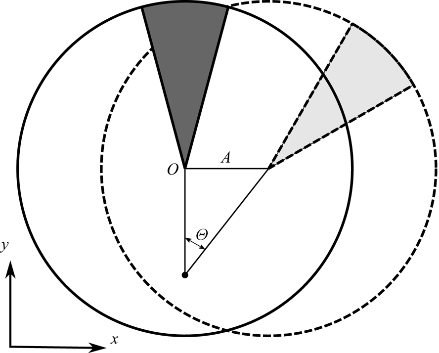
Consider the plane motion of a circular cylindrical wing of radius  $a$, performing simultaneously translational and rotational harmonic oscillations (heaving and pitching) with the same frequency
 $\omega$ and amplitudes
 $A$,
 $\varTheta$, respectively, (see figure 1) in a viscous incompressible fluid. To describe the fluid flow, let us choose a polar coordinate system
 $(r,\theta )$ moving translationally with the centre of the cylinder,
 \begin{equation} x = x_O(t) +r \cos(\theta), \quad y = y_O(t) +r \sin(\theta), \end{equation}
where  $(x, y)$ are coordinates in a fixed inertial Cartesian coordinate system and functions
 $x_O(t) , y_O(t)$ determine the law of translational motion of the centre of the cylinder. We also normalize the spatial variables, time and velocity by
 $a$,
 $\omega ^{-1}$,
 $U = A \omega$, respectively. Using as the main flow characteristics the vorticity
 $w$ and the stream function
 $\psi$ associated with the velocities
 $v_r$,
 $v_ \theta$ of the fluid motion by the relations
 \begin{equation} v_r=\frac{1}{r} \frac{\partial \psi}{\partial \theta},\quad v_\theta={-}\frac{\partial \psi}{\partial r},\quad w ={-}\frac{1}{r}\left(\frac{\partial (r v_\theta)}{\partial r}-\frac{\partial v_r}{\partial \theta}\right), \end{equation}
we write the governing equations in the form
 $$\begin{gather} \frac{\partial w}{\partial t} -\frac{\gamma}{r} \frac{\partial(\psi, w)}{\partial(r,\theta)}=\beta^{{-}1} \varDelta w, \quad w =\varDelta \psi , \end{gather}$$
 $$\begin{gather}\frac{\partial(\psi, w)}{\partial(r,\theta)}=\frac{\partial \psi}{\partial r} \frac{\partial w}{\partial \theta}-\frac{\partial \psi}{\partial \theta} \frac{\partial w}{\partial r}, \end{gather}$$
where  $\varDelta$ is the Laplace operator,
 $\beta$ and
 $\gamma$ are the dimensionless frequency and the amplitude of translational oscillations, respectively. These dimensionless complexes are defined as follows:
 \begin{equation} \beta=\frac{a^2\omega}{\nu}, \quad \gamma=A/a. \end{equation}
Hereinafter,  $\gamma$ will be considered as a small parameter.
Scheme of synchronous rotational–translational oscillations of the cylinder. The dashed line shows the rightmost position of the cylinder and the solid line indicates neutral position. Here  $A$ and
 $\varTheta$ are the amplitudes of translational and rotational oscillations.

We supplement the equations of fluid motion with the following boundary conditions:
 $$\begin{gather} r = 1: \quad \psi = 0, \quad \frac{{\partial \psi }}{{\partial r}} = \xi \cos{t}, \end{gather}$$
 $$\begin{gather}r \to \infty : \quad \psi \sim{-}r\sin{\theta} \cos{t} + u^*_{\infty} r \cos{(\theta+\alpha)}. \end{gather}$$
On the cylinder surface ( $r=1$) the no-slip conditions (2.6) are set. Here
 $\xi$ is the third dimensionless parameter of the problem. It defines the ratio of the amplitudes of rotational (
 $\varTheta$) and translational (
 $A$) oscillations,
 \begin{equation} \xi=a\varTheta/A=\varTheta/\gamma. \end{equation}
The condition (2.7) at infinity consists of two terms. The first one specifies a homogeneous oscillatory flow in the direction of cylinder oscillations (parallel to the  $Ox$ axis). The second term specifies a stationary flow directed at an angle of
 $\alpha$ to the
 $Oy$ axis, it determines the average velocity of the cylinder in the fluid. Further, we will consider the case of a cruising motion. Under conditions of small oscillation amplitudes, the order of cruising speed, obviously, cannot be higher than
 $O(\xi \gamma )$, therefore, we will assume that
 $u^* _{\infty } = u_ {\infty } \xi \gamma$. The values of
 $u_{\infty }$ and
 $\alpha$ will be considered as unknown and determined from the condition that the time-average forces acting on the cylinder are equal to zero.
2.2. Force characteristics
Let us define the hydrodynamic forces  $f_x, f_y$ and the moment
 $m$ acting per unit length of the cylinder. Normalizing the forces to
 $f_{sc} = 2 {\rm \pi}\rho a^2U \omega$ (where
 $\rho$ is the density of the fluid), the moment to
 $a f_{sc}$, we represent them in terms of vorticity as (e.g. Dynnikova & Andronov Reference Dynnikova and Andronov2018)
 \begin{equation} \left. \begin{array}{c@{}}
\displaystyle f_y-if_x
=\dfrac{i}{2}\sin{t}+\dfrac{1}{2{\rm \pi}\beta}\int_0^{2{\rm \pi}}\left(\dfrac{\partial
w}{\partial r}-w\right)_{r=1}\, {\rm e}^{{\rm i}\theta}
\,{\rm d} \theta,\\ \displaystyle m =\dfrac{2
\xi}{\beta}\cos{t}-\dfrac{1}{2{\rm \pi}\beta}\int_0^{2{\rm \pi}}(w)_{r=1}
\,{\rm d} \theta. \end{array}\right\}
\end{equation}
The first term in (2.9a) is the Krylov–Froude force, which appears as a result of the transition to a moving coordinate system. The terms proportional to  $w$ and
 $\partial {w} / \partial r$ represent the contributions of the shear stresses and pressure, respectively.
The forces and moments are used to determine the time-average energy dissipation. Normalized to  $D{sc} = U f_{sc}$, it can be written as
 \begin{equation} \left. \begin{array}{c@{}} d =d_x+\xi^2 d_\theta,\\ d_x={-}\langle f_x(t) \cos{t}\rangle, \quad d_\theta=\xi^{{-}1}\langle m(t) \cos{t}\rangle. \end{array}\right\} \end{equation}
Angle brackets hereinafter denote averaging over the oscillation period. The sign in the expression for  $d_\theta$ is determined by the fact that the angular velocity of rotation of the cylinder is
 $-\xi \cos {t}$.
3. Asymptotic solution
3.1. Expansion in the small parameter
Without making any assumptions about the parameter  $\beta$, let us assume that
 $\gamma \ll 1$ and
 $\xi \sim 1$. We will construct a solution of the problem in the form of a series in powers of
 $\gamma$, limiting ourselves to the first two terms,
 \begin{equation} \psi = {\psi ^{(0)}} + \gamma {\psi ^{(1)}} + \cdots ,\quad w = {w^{(0)}} + \gamma {w^{(1)}} + \cdots . \end{equation}
In the leading term, we obtain the Stokes approximation of the original problem:
 \begin{equation} \left. \begin{array}{c@{}}
\dfrac{\partial }{{\partial t}}{w^{(0)}} - {\beta ^{ -
1}}\varDelta {w^{(0)}} = 0,\quad {w^{(0)}} = \varDelta {\psi
^{(0)}};\\ r = 1:\quad \psi^{(0)} = 0, \quad
\dfrac{{\partial \psi^{(0)} }}{{\partial r}} = \xi \cos{t},
\quad r \to \infty : \quad \psi^{(0)} \sim{-}\cos{t}\cdot
r\sin{\theta}. \end{array}\right\}
\end{equation}
The Stokes solution of the problem describes a purely periodic motion of a fluid.
For the next term we have
 \begin{equation} \left. \begin{array}{c@{}}
\dfrac{\partial }{{\partial t}}{w^{(1)}} - {\beta ^{ -
1}}\Delta {w^{(1)}} = {G},\quad {w^{(1)}} = \Delta {\psi
^{(1)}},\quad {G} = \dfrac{1}{r}
\dfrac{\partial(\psi^{(0)}, w^{(0)})}{\partial(r,\theta)};
\\ r = 1:\quad \psi^{(1)} =\dfrac{{\partial \psi^{(1)}
}}{{\partial r}} = 0, \quad\quad r \to \infty : \quad
\psi^{(1)} \sim \xi u_\infty r \cos{(\theta+\alpha)}.
\end{array} \right\} \end{equation}
The solution of the second subproblem contains both periodic and stationary components. The latter is often called secondary flow or steady streaming. As will be shown below, steady streaming, in the considered case of rotational–translational oscillations, provides the directed motion of the cylinder in the fluid.
3.2. Stokes approximation
In the Stokes approximation, the linear problem (3.2) splits into two. The first of them is the problem of an oscillatory fluid flow around a fixed cylinder, the second is the problem of rotational oscillations of a cylinder in an undisturbed fluid. Accordingly, the total flow is represented as the sum of these two flows
 \begin{equation} \left. \begin{array}{c@{}} \psi^{(0)}= \sin{\theta} \mathrm{Re} ( \varPsi_{1}(r) \, {\rm e}^{{\rm i}t}) +\xi \mathrm{Re} ( \varPsi_{2}(r) \, {\rm e}^{{\rm i}t}),\\ w^{(0)}=\sin{\theta}\, \mathrm{Re} ( W_{1}(r) \, {\rm e}^{{\rm i}t})+\xi \mathrm{Re} ( W_{2}(r) \, {\rm e}^{{\rm i}t}). \end{array}\right\} \end{equation}
The solutions of the corresponding one-dimensional problems are
 \begin{equation} \left. \begin{array}{c@{}} {\varPsi _1} ={-}r +\dfrac{1}{r}+\dfrac{S_x}{r} + {z^{ - 2}}{W_1},\quad {W_1} ={-}2z \dfrac{{{K_1}({z r})}}{{{K_0}({z})}}, \quad S_x(z) = \dfrac{{2{K_1}({z})}}{{{z}{K_0}({z})}},\\ {\varPsi _2} = S_\theta + { z^{ {-}2}}{W_2},\quad {W_2} ={-}z \dfrac{{{K_0}({z r})}}{{{K_1}(z)}},\quad S_\theta(z) = \dfrac{{{K_0}({z })}}{{{z}{K_1}({z})}}, \quad z =\sqrt{i \beta}. \end{array}\right\} \end{equation}
Here  $K_j$ are modified Bessel functions. As can be seen, outside the Stokes boundary layer with a thickness of the order of
 $\beta ^{-1/2}$, the vorticity (its
 $W_1$ and
 $W_2$ components) decays exponentially and the flow becomes potential. Additional viscous terms
 $S_x r^{- 1}$ and
 $S_\theta$, which disappear in an effectively inviscid fluid (at
 $\beta = \infty$), correct the non-circulation flow of an ideal fluid outside the boundary layer.
Based on the obtained solution, it is possible to determine the hydrodynamic forces and moment acting on the cylinder and the time-average energy dissipation (in the first approximation):
 \begin{equation} \left. \begin{array}{c@{}} f^{(0)}_x= \text{Im} \left[{\rm e}^{{\rm i}t}\left(\dfrac{1}{2}+S_x\right)\right], \quad m^{(0)}=\dfrac{2 \xi}{\beta}\cos{t}-\xi \text{Im} [{\rm e}^{{\rm i}t}(S_\theta)],\\ \quad d^{(0)}_x={-}\dfrac{1}{2} \text{Im} [S_x], \quad d^{(0)}_\theta=\dfrac{1}{\beta}-\dfrac{1}{2} \text{Im} [S_\theta]. \end{array} \right\} \end{equation}
For  $\beta = \infty$ (effectively inviscid fluid) functions,
 $S_x = S_\theta =0$ vanish, therefore the moment and force acting on the cylinder are purely inertial. They are proportional to the angular and linear acceleration of the cylinder with the added mass coefficients equal to
 $1/2$. For
 $\beta <\infty$, additional force components appear. They are completely determined by the functions
 $S_x(z)$ and
 $S_\theta (z)$.
In the practically important case of large  $\beta$, the behaviour of
 $S_x(z)$ and
 $S_\theta (z)$ is described by the asymptotics
 \begin{equation} z \to \infty: \begin{array}{c} S_\theta(z) \sim \dfrac{1}{z}-\dfrac{1}{2z^2}+\dfrac{3}{8z^3}-\dfrac{3}{8z^4}+O(z^{{-}5}),\\ S_x(z) \sim \dfrac{2}{z}+\dfrac{1}{z^2}-\dfrac{1}{4z^3}+\dfrac{1}{4z^4}+O(z^{{-}5}). \end{array} \end{equation}
Substituting (3.7) into (3.6) we obtain the following expansion of functions  $d_x$,
 $d_\theta$ for large values of
 $\beta$:
 \begin{equation} \beta \to \infty: \begin{array}{c} d^{(0)}_{\theta }=\dfrac{\beta^{{-}1/2}}{2 \sqrt{2} }+\dfrac{3 \beta^{{-}1}}{4}+\dfrac{3\beta^{{-}3/2}}{16 \sqrt{2} }+O(\beta^{{-}5/2}),\\ d^{(0)}_x=\dfrac{\beta^{{-}1/2}}{\sqrt{2}}+\dfrac{\beta^{{-}1}}{2 } -\dfrac{\beta^{{-}3/2}}{8 \sqrt{2}}+O( \beta^{{-}5/2}). \end{array} \end{equation}
3.3. Secondary flow problem
Let us define the first-order terms in the asymptotic representation (3.1a,b). We will be interested only in their stationary components, which describe the steady streaming. The same components should be kept on the right-hand side  $G$ of (3.3). Separating them, we get
 \begin{equation} \langle G \rangle =G_x\sin{2\theta}+\xi G_\theta \cos\theta, \end{equation}
where
 \begin{equation} G_x= \frac{1}{4r} \mathrm{Re} ( \bar{W}_1\varPsi'_1-\bar{\varPsi}_1W'_1), \quad G_\theta=\frac{1}{2r} \mathrm{Re} (\bar{W}_1\varPsi'_2 -\bar{\varPsi}_1W'_2). \end{equation}
Here and below, the overbar denotes the complex conjugation, and the prime mark denotes the derivative with respect to  $r$. Carrying out direct calculations and using the notation
 \begin{equation} \varPhi_k(r;\beta)=\frac{K_k(\sqrt{i\beta}r)}{K_k(\sqrt{i\beta})}, \quad S(\beta)=\frac{K_2(\sqrt{i\beta})}{K_0(\sqrt{i\beta})}, \end{equation}
we get
 $$\begin{gather} G_x(r;\beta) = \frac{\beta}{2} {\text{Im}}\left(\frac{\bar{S}\varPhi_0}{r^2}+2S\varPhi_2 \overline{\varPhi}_0-S\varPhi_2 \right), \end{gather}$$
 $$\begin{gather}G_\theta (r;\beta) = \frac{\beta}{r}{\text{Im}} (S)|\varPhi_1|^2 -\frac{\beta}{2}{\text{Im}} ( ( 1- \bar{S}r^{{-}2}) \varPhi_1). \end{gather}$$
Finding the solution of (3.3) in the form
 \begin{equation} {\psi^{(1)}} = \varPsi_x(r)\sin{2\theta}+\xi\varPsi_\theta(r)\cos\theta, \end{equation}
we obtain the following problems for  $\varPsi _x$ and
 $\varPsi _\theta$:
 $$\begin{gather} {\mathcal{L}}_2^2{\varPsi_x}={-}\beta {G_x}, \quad {\mathcal{L}}_1^2{\varPsi_\theta}={-}\beta {G_\theta}, \quad {\mathcal{L}}_k= \frac{1}{r}\frac{{\rm d}}{{\rm d} r}r\frac{{\rm d}}{{\rm d} r} - \frac{k^2}{r^2}, \end{gather}$$
 $$\begin{gather}r = 1:\ {\varPsi_x} ={\varPsi'_x}= {\varPsi_\theta} ={\varPsi'_\theta}=0, \quad r \to \infty :\ \varPsi'_x=0 , \quad \varPsi'_\theta = u_\infty. \end{gather}$$
The right-hand sides of (3.15a,b) decrease exponentially with increasing  $r$. As a consequence, there are unique solutions
 $\tilde {\varPsi }_x$,
 $\tilde {\varPsi }_\theta$ of the inhomogeneous (3.15a,b) that exponentially decrease as r goes to infinity. Using the method of variation of an arbitrary constant (details are given in Appendix A), they can be represented in the following integral form:
 \begin{align} \tilde{\varPsi}_x={-}\frac{\beta r^4}{48}\int_1^\infty G_x(rx)( x^2-1 )^3 \frac{{\rm d}\kern0.06em x}{x}, \quad \tilde{\varPsi}_\theta={-}\frac{\beta r^4}{16}\int_1^\infty G_\theta(rx)( x^4-4x^2\ln{x}-1)\,{{\rm d}\kern0.06em x}. \end{align}
Adding to  $\tilde {\varPsi }_x$,
 $\tilde {\varPsi }_\theta$ general solutions of homogeneous equations, we get
 \begin{align} \varPsi_x= \tilde{\varPsi}_x-\frac{B_x}{r^2}+C_x\left( 1-\frac{1}{r^2}\right),\quad \varPsi_\theta= \tilde{\varPsi}_\theta-\frac{B_\theta}{r}+C_\theta\left( r-\frac{1}{r}\right) +D\left( r\ln{r}-\frac{r}{2} + \frac{1}{2r}\right). \end{align}
The boundary conditions for  $r = 1$ are satisfied by choosing arbitrary constants
 $B_{x, \theta }$,
 $C_{x, \theta }$:
 \begin{equation} B_{x,\theta}=\tilde{\varPsi}_{x,\theta}(1), \quad C_\theta={-}\frac{\tilde{\varPsi}'_\theta(1)+\tilde{\varPsi}_\theta (1)}{2},\quad C_x={-}\frac{\tilde{\varPsi}'_x(1)+2\tilde{\varPsi}_x(1)}{2}. \end{equation}
The function  $\varPsi _x$ goes to the constant
 $C_x$ as
 $r \to \infty$. This does not contradict the boundary conditions at infinity. The function
 ${\varPsi }_\theta$ has the classical logarithmic singularity at infinity. It is impossible to determine the constant
 $D$ and satisfy the condition for the stream function at
 $r \to \infty$ for an arbitrary velocity of a stationary flow without taking into account the convective terms (Stokes’ paradox). Only with a special choice of
 $u_\infty$ and
 $\alpha$,
 \begin{equation} u_\infty=C_\theta(\beta),\quad \alpha=0, \end{equation}
is the condition at infinity satisfied, and the constant  $D$ vanishes. It turns out that this choice exactly corresponds to the cruising motion condition, that the force averaged over the period, acting on the body from the fluid, is equal to zero.
This can be shown by calculating, according to (2.9), the contributions to the force  $f_y$ from the four terms of
 ${\varPsi }_\theta$ in (3.18b). The second and third do not generate vorticity, and therefore do not make any contribution. The contribution from the first term, up to a factor, is determined by the integral (Appendix A)
 \begin{equation} \int_1^\infty G_\theta (x;\beta) x^2 {{\rm d}\kern0.06em x} =0, \end{equation}
the explicit calculation of which also gives zero. The contribution of the last term is  $D$. To fulfil the cruise flight condition we must set
 $D = 0$. Therefore, the last term in (3.18b) should be discarded. In this case, the cylindrical wing will move along the
 $Oy$ axis with a cruising speed
 $\xi \gamma C_\theta$.
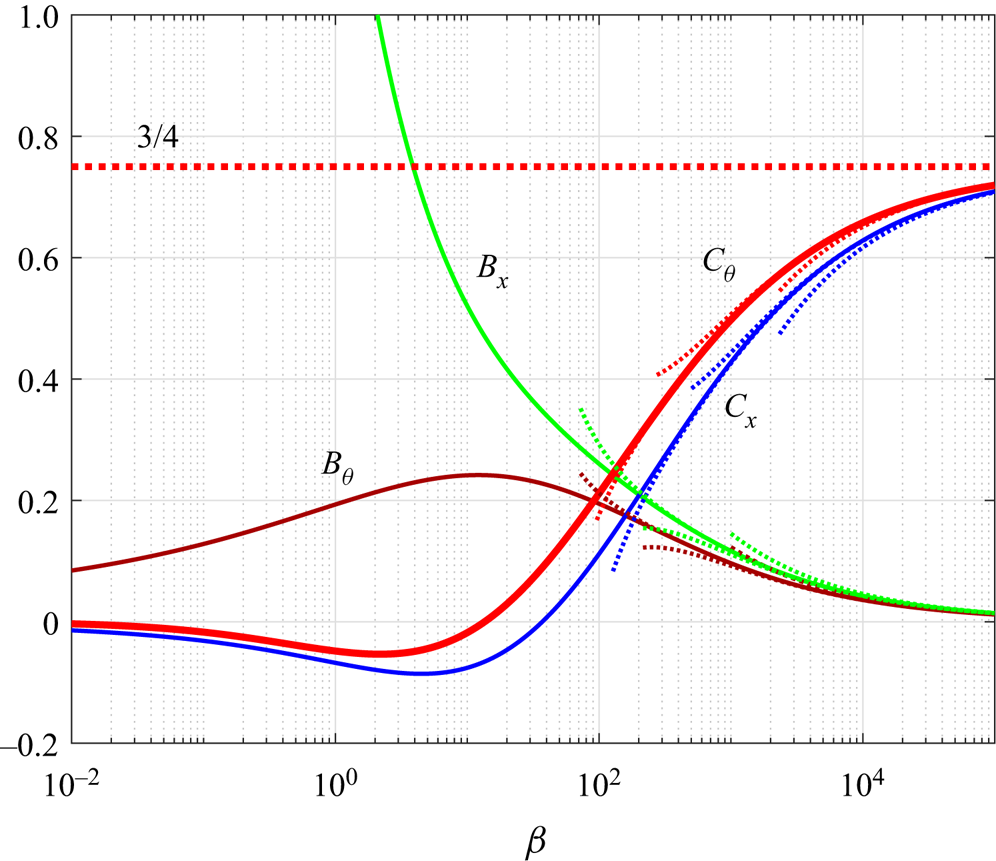
The change of the cruising speed coefficient  $u_\infty = C_\theta$ depending on dimensionless frequency
 $\beta$ is shown in figure 2. The obtained results show the presence of two types of cruising motion of the cylinder: forward (
 $u_\infty >0$) and reverse (
 $u_\infty <0$). The first of them is realized for
 $\beta > \beta _\theta = 13.5355$ and is characterized by a monotonic growth of the cruising speed with increasing frequency
 $\beta$. The maximum speed of such a motion is
 $3/_4\gamma \xi U=3/_4\varTheta U$, which is comparable to the amplitude of the velocity
 $U$ of translational oscillations of the cylinder. The reverse motion occurs when
 $\beta <\beta _\theta$. The cruising speed coefficient reaches the smallest value
 $u_\infty = -0.0534$ at
 $\beta = 2.18$. This value is more than an order of magnitude less than the maximum value of the cruising speed coefficient,
 $u_\infty = 0.75$, of direct motion.
Dependence of the main integral characteristics on the dimensionless frequency  ${\beta }$. Dashed lines represent asymptotics of different orders.

For the case  $\beta \to \infty$,
 $u_\infty (\beta )$ is determined by the following asymptotic relationship:
 \begin{equation} u_\infty = C_\theta = \frac{3}{4}-7\sqrt{2}\beta^{{-}1/2}+\frac{1117}{16}\beta^{{-}1}- \frac{3183}{8\sqrt{2}}\beta^{{-}3/2}+O( \beta^{{-}2}). \end{equation}
The asymptotic behaviour of other main integral characteristics of the steady streaming at high oscillation frequencies is determined by the formulae
 $$\begin{gather} C_x = \frac{3}{4}-\frac{603}{32\sqrt{2}}\beta^{{-}1/2}+\frac{3681}{32} \beta^{{-}1}-\frac{405159}{512\sqrt{2}}\beta^{{-}3/2}+O( \beta^{{-}2}), \end{gather}$$
 $$\begin{gather}B_x = \frac{13}{2\sqrt{2}}\beta^{{-}1/2}-\frac{137}{4}\beta^{{-}1} +\frac{3963}{16\sqrt{2}}\beta^{{-}3/2}+O( \beta^{{-}2}), \end{gather}$$
 $$\begin{gather}B_\theta = \frac{11}{2\sqrt{2}}\beta^{{-}1/2}-\frac{123}{4}\beta^{{-}1} +\frac{2957}{16\sqrt{2}}\beta^{{-}3/2}+O( \beta^{{-}2}). \end{gather}$$
The asymptotics for  $\beta \to \infty$ are shown by dashed lines in figure 2 together with the exact solution (solid lines). Table 1 also shows the boundaries of their range of applicability, which were estimated as the values of
 $\beta$ at which the relative approximation error reaches 5 %.
The limits of applicability of asymptotics of various order of  $n$ with respect to the parameter
 $\beta$. The values (of
 $\beta$) in the table are given for the case when the error of the asymptotics reaches 5 %.

4. Flow regime map
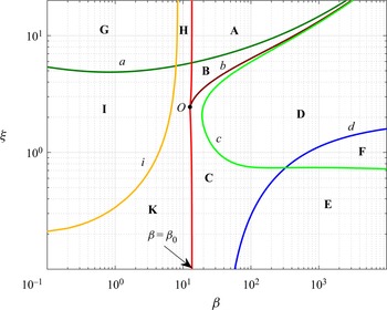
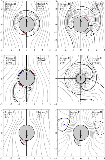
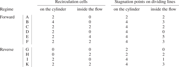
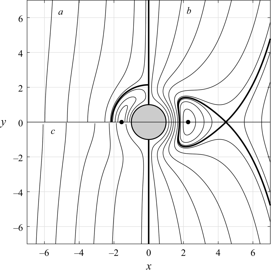
Let us analyse the structure of the secondary flows described by the solution (3.14). Each of the two types of cruising motion of the cylinder (forward and reverse) correspond to their own set of regimes of steady streaming. The classification of the regimes of steady streaming in the parametric plane  $(\beta, \xi )$ was carried out according to the number and type of stagnation points, where the flow velocity vanishes (more information on this approach can be found in the works of Perry & Chong (Reference Perry and Chong1987) and Bhosale, Parthasarathy & Gazzola (Reference Bhosale, Parthasarathy and Gazzola2020)). Two types of such points were distinguished: the centres of the recirculation cells (RC) ( the cells can be attached to the cylinder or located inside the flow) and stagnation points on dividing lines, such as separation points or reattachment points (they can be located on the cylinder or inside the flow). Analysis of the flow patterns makes it possible to identify 10 main regimes of steady streaming: six for forward and four for reverse motion of the cylinder. Their characteristics are given in table 2, the flow regime map is plotted in figure 3, the streamline patterns in the half-plane (all regimes are symmetric about the
 $Oy$ axis) are shown in figure 4. We call these regimes basic, separating them from transitional regimes that are realized in a narrow vicinity of the critical point
 $\beta _\theta$, where the direction of the cylinder's motion changes. This narrow area in figure 3 is indistinguishable from the straight line
 $\beta = \beta _\theta$. These regimes, in contrast to the basic ones, are, in our opinion, only of academic interest. For completeness, information about them is provided in Appendix C. Various flow regimes A–K in the diagram in figure 3 are separated from each other by curves
 $a$–
 $i$. Let us consider their characteristics.
Map of the main flow regimes A–K in the parametric plane  $(\xi,\beta )$. The corresponding flow patterns are shown in figure 4.

Streamlines of secondary flows in the basic regimes of forward and reverse motion. Bold lines represent dividing streamlines, black markers on them indicate stagnation points. Coloured markers indicate the centres of the RC. Arrows show the direction of propulsive motion ( $\uparrow$ forward and
 $\downarrow$ reverse).

Classification of the main regimes of steady streaming around a cylinder performing synchronous rotational–translational oscillations.

In regimes A, H and G that are above the curve  $a=(\xi _a,\beta _a)$, there are two stagnation points on the cylinder, located at
 $\theta = \pm {\rm \pi}/2$. For regimes below the curve
 $a$ on the cylinder there are two more stagnation points (in addition to the two indicated ones), the positions of which are determined by the relation
 $\sin {\theta } = -\xi /\xi _a$. In the H mode of reverse motion, there are RC of finite dimensions inside the flow region. During the transition (see figure 3) to regime G, the centres of these cells go to infinity. When the flow at
 $\beta = \beta _0$ passes into regime A of direct motion, RC become infinite in size, occupying the entire flow region. For
 $\beta > \beta _0$ (in regime A) cells remain attached to the cylinder, completely enclosing its surface, their size decreases from infinity (at
 $\beta = \beta _0$) to zero (for
 $\beta \to \infty$). The curve
 $i=(\xi _i,\beta _i)$ at
 $\xi \to \infty$ turns into a straight line
 $\beta _- = 8.35$. Regimes G, H, A in the limit
 $\xi \to \infty$ become subcritical, intermediate and supercritical flow regimes (see Appendix B).
In forward motion, when  $\xi$ decreases below
 $\xi _a$, regime A transforms into regime B, which is characterized by the formation of a second pair of small attached RC inside the main pair of attached RC enclosing the cylinder (see figure 4). As
 $\xi$ decreases, the size of the small cells grows, and when reaching the curve
 $b=( \xi _b, \beta _b)$, they detach from the cylinder and separate from the large cells, turning into a pair of isolated inner RC (see regime C in figure 4). The curve
 $b$ (the border between B and C regimes) starts at the point
 $O$ (
 $\beta _O = 12.65$,
 $\xi _O = 2.45$) and merges with the curves
 $a$ and
 $c$ at
 $\beta \to \infty$.
The curve  $c = (\xi _c,\beta _c)$ separates the regimes C and D, E and F. This curve starts at the point
 $\xi = 0, \beta = \beta _+ = 37.064$ and ends at the point
 $\xi = 2$,
 $\beta = \infty$. When passing through the line
 $d$ from D to F on the line
 $\theta = - {\rm \pi}/2$ of symmetry, a pair of inner cells adjoining along the line of symmetry appears and grows inside the flow. As
 $\beta$ increases, the pair of cells approach the cylinder at a distance of the order of the thickness
 $\beta ^{- 1/2}$ of the boundary layer. The same thing happens when the flow is transformed from regime C to regime E. In this case, the inner isolated RC of regime C are pressed by a new pair of RC closer to the cylinder. With an increase of
 $\beta$, isolated RC become part of the boundary layer of thickness
 $\beta ^{- 1/2}$ on the surface of the cylinder. The limiting cases
 $\beta \to \infty$ and
 $\xi \to 0$ are considered in detail in Appendix B.
In the region  $\xi <\xi _a$, two regimes of reverse motion of the cylinder I and K are realized. When passing from G to I and from H to K through the boundary
 $a$, two RC attached to the cylinder appear. With the subsequent decrease of
 $\xi$, the size of these cells grows. When passing from I to K through the
 $i$ boundary, a pair of point cells appears inside the flow region. With the subsequent decrease of
 $\xi$ in regime K, a pair of inner RC grows to infinite size. The outer boundaries of RC attached to the cylinder also go to infinity.
The transition between regimes A, B and C of the forward motion and H, K of the reverse motion of the cylinder occurs in a narrow zone near the critical value  $\beta _0$ of the dimensionless frequency. The flow regimes in this zone are briefly discussed in Appendix C.
5. Analysis of results
5.1. The limits of applicability of the asymptotic theory
To investigate the limits of applicability of the asymptotic theory, we carried out a numerical simulation of the flow past a flapping cylindrical wing. A numerical solution was constructed for the full problem (2.3)–(2.7) using the finite volume method. For this purpose, the numerical scheme developed in Nuriev, Kamalutdinov & Egorov (Reference Nuriev, Kamalutdinov and Egorov2019); Nuriev et al. (Reference Nuriev, Egorov and Kamalutdinov2021) was used. The details of the simulations are described in Appendix D.
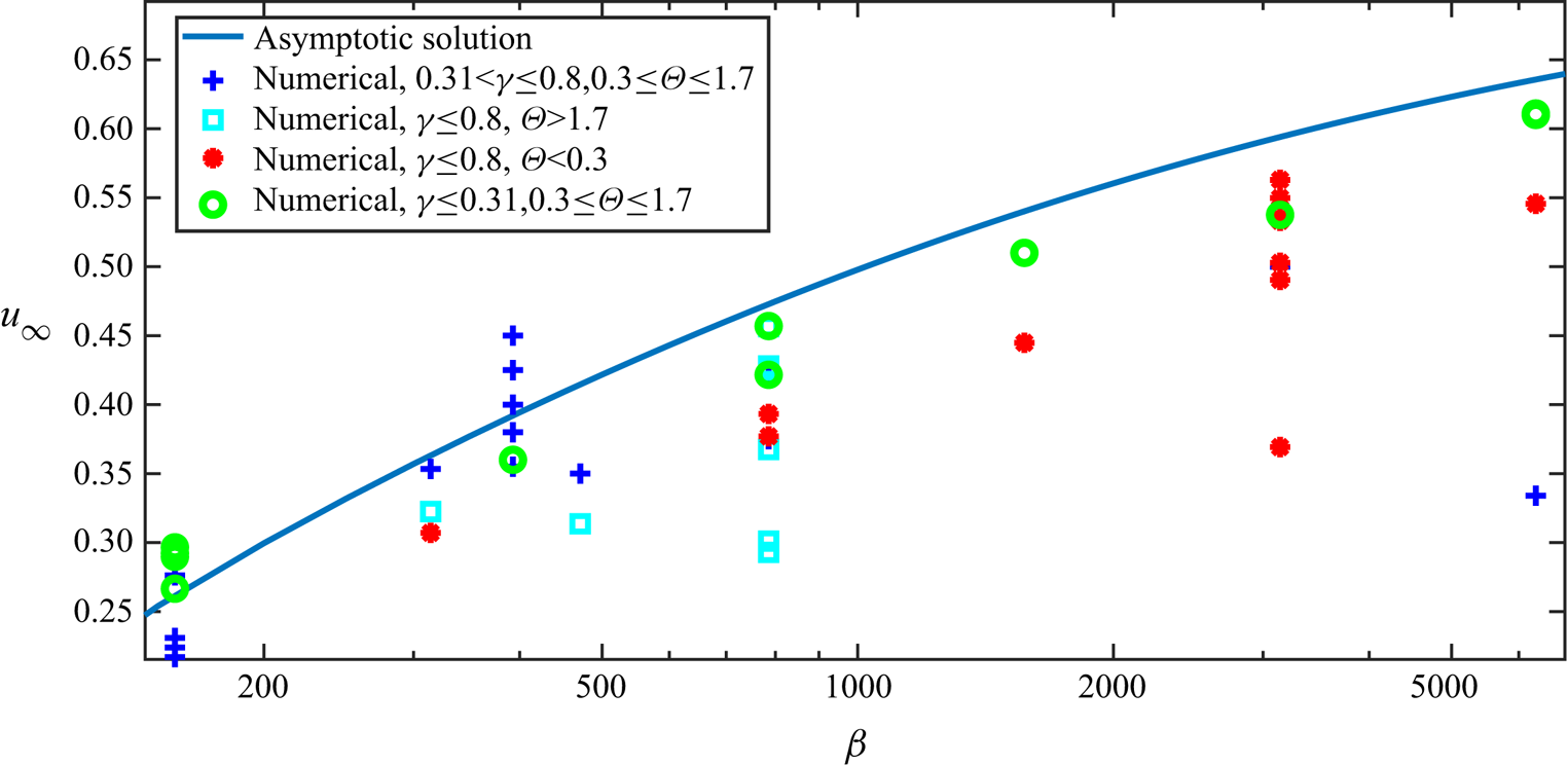
In figure 5 a graph of the asymptotic dependence of cruising speed coefficient on frequency and the numerical simulation data obtained in the range of parameters  $150 <\beta <6500$,
 $0.031 <\gamma <0.8$,
 $0.4 \leq \xi \leq 15$ are presented. As one can see, the values of the velocity coefficient obtained numerically for the same frequency
 $\beta$ change depending on the values of
 $\gamma$ and
 $\varTheta = \xi \gamma$. Recall here that in the framework of the asymptotic expansion, only the main stationary term was found, which determines the cruising speed as a linear function of
 $\varTheta$. The next terms of the asymptotic expansion define corrections proportional to higher powers of
 $\varTheta$ and
 $\gamma$ (and their combinations), which start to play a significant role as the amplitudes of rotational and translational oscillations increase (for this reason, for relatively large values of
 $\varTheta$ and
 $\gamma$, there is no single universal similarity parameter). The deviation of the numerical data from the linear (in relation to
 $\varTheta$) asymptotic approximation just indicates the magnitude of nonlinear corrections for different values of
 $\varTheta$ and
 $\gamma$.
Dependence of the cruising speed coefficient  $u_\infty$ on the dimensionless frequency
 $\beta$. The asymptotic solution is shown by the solid line, the numerical results are indicated by markers.

Nevertheless, the dependence of cruising speed coefficient on frequency predicted by the main stationary term of asymptotic model is well traced in the entire designated range of parameters. At moderate frequencies  $150 \leq \beta \leq 470$, most of the numerical results have minimal deviations (
 $\pm 12\,\%$) from the theoretical dependence. In the high-frequency region
 $\beta > 470$, the asymptotics determines the upper values of the velocity coefficient (which are achieved at low values of
 $\gamma$).
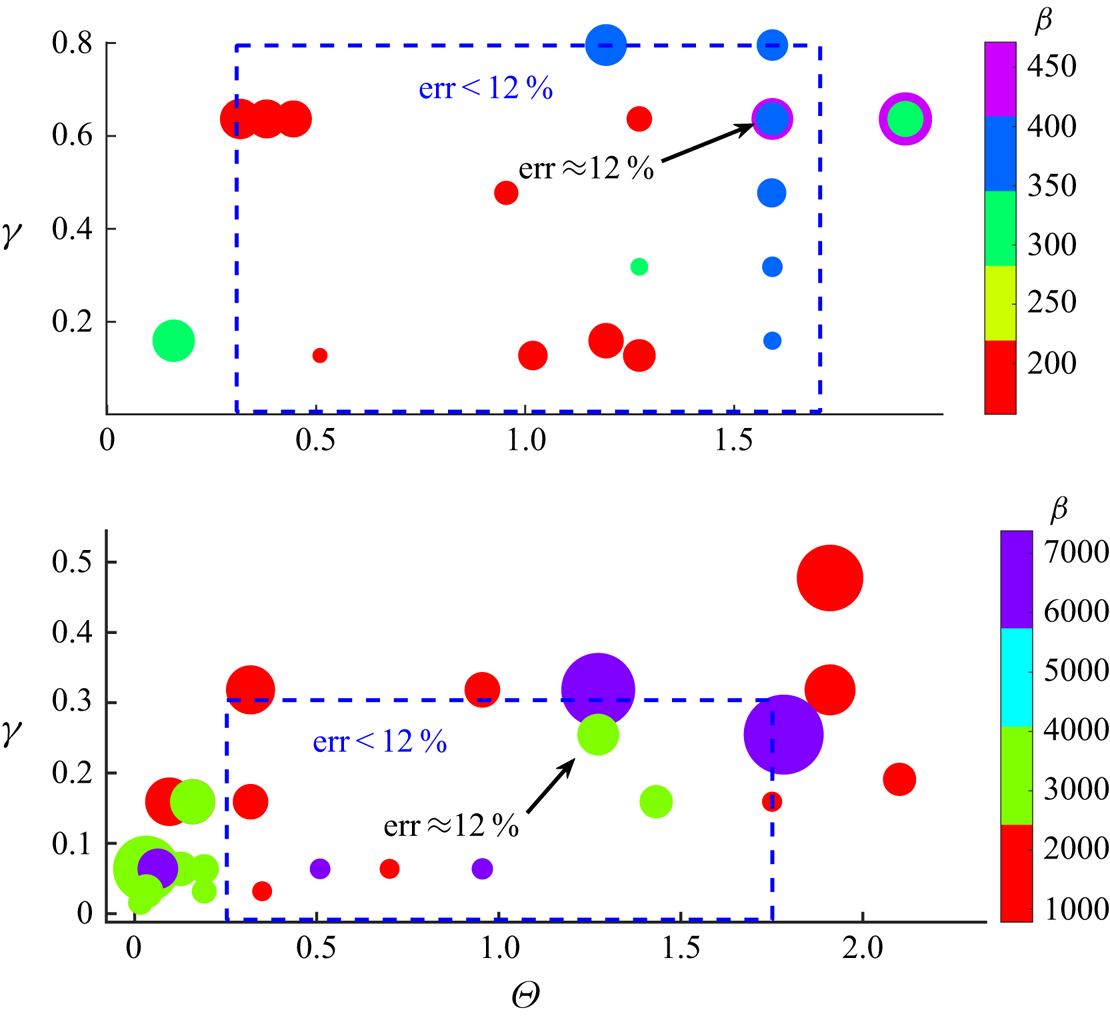
The deviations  $err = |1-u^{num}_\infty /u_\infty | \cdot 100\,\%$ of numerical values of the speed coefficient
 $u^{num} _ \infty$ from the theoretical curve
 $u_\infty (\beta )$ for different values of
 $\gamma$ and
 $\varTheta$ are shown in the bubble plots in figure 6 (each marker in figure 5 corresponds to a bubble in figure 6). The size of the bubble indicates the magnitude of deviation value (a large size corresponds to a large deviation), the coordinates show the values of
 $\gamma$ and
 $\varTheta$, the colour indicates the value of
 $\beta$. This representation of data allows one to identify parametric regions with minimal deviations between analytical and numerical results, which can be considered as the areas of applicability of the theory.
Deviations  $err = |1-u^{num}_\infty / u_\infty |\times 100$ of numerical values of the cruising speed from the theoretical ones depending on the parameters
 $\gamma, \varTheta, \beta$. The size of the marker (bubble) indicates the magnitude of deviation value, the colour indicates the value of
 $\beta$ (see the colour map).

In the diagrams (figure 6), blue rectangles indicate areas where the deviations  $err$ did not exceed 12 % for all values of
 $\beta$ in the indicated ranges. As you can see, for moderate-frequency oscillations, the asymptotic model has a very wide range of applicability:
 $0<\gamma \leq 0.8$,
 $0.3 \leq \varTheta < 1.7$. Here the theory is valid for cases when the amplitude of translational oscillations does not exceed
 $4/5$ of the radius, and the angle of rotation is not more than
 $98^{\circ }$ and not less than
 $17^{\circ }$. The lower constraints on the parameter
 $\varTheta$ are obviously related to the specificity of the interaction between translational and rotational oscillations at small angles of rotation. The theory can be applied in the range
 $\varTheta < 0.3$ for relatively large values of
 $\xi$, however, detailed calculations to identify the exact dependences in this narrow range have not been performed. In the region of high values of the dimensionless frequency, the limits of applicability of the theory in terms of the amplitudes
 $\gamma$ significantly decrease: here the deviation
 $err<12\,\%$ is observed for
 $\gamma \leq 0.3$ (see figure 6).
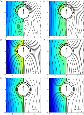
The accuracy of the cruising speed determination (in the areas of applicability) is undoubtedly related to the accuracy with which the asymptotic theory in the obtained approximation can describe the structure of the flow. Figure 7 shows comparisons between the flow patterns of secondary streaming obtained analytically (right-hand side of the image) and numerically (left-hand side of the image). The visualization is presented for  $\beta = 157$, where the structural features of the flows are most clearly distinguishable (all RC are of a sufficiently large size). According to the asymptotic theory (see § 4), the flow structure depends only on the parameter
 $\xi$. At a given frequency, this parameter varied in the range
 $0.46 \leq \xi \leq 11$. The values of the second parameter
 $\gamma$ in the calculations were selected so as to be within and on the boundaries of the selected applicability area.
Flow patterns of secondary streaming obtained analytically (right-hand black and white part of the image) and numerically (left-hand half of the image) for  $\beta =157$ and
 $\gamma =0.64$,
 $\xi = 0.46$ (a),
 $\gamma =0.64$,
 $\xi = 0.72$ (b),
 $\gamma =0.64$,
 $\xi = 2$, (c),
 $\gamma =0.13$,
 $\xi = 4$, (d),
 $\gamma =0.16$,
 $\xi = 7.5$ (e),
 $\gamma =0.16$,
 $\xi = 11$ ( f). Arrows show the direction of propulsive motion. The values of
 $err$ indicate the deviation of the numerical values of the cruising speed from the theoretical ones.

In the largest part of the computational domain  $0.72 \leq \xi \leq 7.5$, regime D was localized; its boundaries are in good agreement with the asymptotic theory (see the flow regime map). As you can see in figure 7(c,d), in this regime the asymptotic model well predicts the changes in the size and position of RC in the flow region depending on the parameter
 $\xi$. This is also reflected in the estimates of the cruising speed: at the interior points
 $\xi = 2, 4$, the values of
 $err$ (see also figure 6) are minimal and equal to
 $err = 5.57, 1.92$, respectively. Note that the calculation for
 $\xi = 2$ was performed at
 $\gamma = 0.64$, i.e. when a peak-to-peak amplitude of translational oscillations is 1.28 times greater than the cylinder radius.
Changes of the flow structure near the lower boundary of regime D are shown in figure 7(a,b) for  $\xi =0.46, 0.72$ and
 $\gamma =0.64$. According to the flow regime map, these points are located in the transition zones between regimes D and E. The features of the flow transformations in the wake of the body, observed in numerical calculations, are somewhat different from the structural changes predicted by the asymptotic theory. As can be seen in figure 7(a) at
 $\xi = 0.46$ in regime E, four external RC should be observed in the wake, in fact (according to the results of numerical calculations) only two cells of a larger size are formed. According to the classification proposed in § 4, the observed regime is of type F, not E. When passing from the case in figure 7(b) to the case figure 7(c),
 $err$ values increase from 11.7 to 16.9, thus, we reach the lower limit of applicability of the theory for the parameter
 $\varTheta$.
In figure 7(e, f) the changes in the flow occurring at large values of  $\xi = 7.5, 11$ are shown. According to the theory, in this parametric range, the flow is transformed from regime D to regime A: a pair of RC located in the front part of the cylinder for smaller
 $\xi$ enclose the entire cylinder. As can be seen, the numerical results confirm such structural changes. However, the sizes of the attached cells predicted by the numerical and analytical models are different. This is directly reflected in the values of
 $err$, which begin to increase in regime A. This is how the upper bound of the region of applicability of the theory in the parameter
 $\varTheta$ is reached.
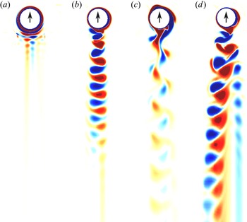
Let us consider the changes in the flow structure when approaching the upper limit of applicability in terms of the oscillation amplitude  $\gamma$, for this we analyse the vorticity field. In figure 8(a) the instantaneous flow pattern in regime D is shown (the dynamics of the flow is presented in the supplementary movies which are available at https://doi.org/10.1017/jfm.2022.287). As you can see, the vortex wake formed behind the body dissipates very quickly. Away from the body, (which is confirmed by the analytical solution) an ideal fluid flow is observed. In the vicinity of the boundary of the applicability range (figure 8b,c), vortex streets are formed behind the body, they decay more slowly than the vortex wake in regime D. Depending on
 $\beta$, the cruising speed in these regimes differs by 10 %–20 % from the theoretical one. In the case in figure 8(b) the speed is lower than the theoretical one, and in the case in figure 8(c) it is higher. A vortex street in the form in figure 8(c) was observed only in the range of moderate values of
 $\beta$. With a further increase of the amplitude
 $\gamma$, the flow loses symmetry about the
 $Oy$ axis (this type of stability loss of a symmetric flow behind a flapping wing was discussed in detail by Dynnikova et al. (Reference Dynnikova, Dynnikov, Guvernyuk and Malakhova2021)). As a result, an additional stationary component of hydrodynamic force arises, acting parallel to the
 $Ox$ axis. The cruising speed in this mode in the direction of
 $Oy$ is no more than
 $2/3$ of the theoretical.
Vorticity field. Instantaneous flow patterns for (a)  $\beta =785$,
 $\varTheta =1.75, \gamma =0.16$; (b)
 $\beta =785$,
 $\varTheta =1.9, \gamma =0.48$; (c)
 $\beta =393$,
 $\varTheta =1.59, \gamma =0.8$; (d)
 $\beta =785$,
 $\varTheta =1.9, \gamma =0.64$. Arrows show the direction of propulsive motion.

5.2. Propulsive efficiency
As already shown above, the considered propulsive mechanism makes it possible to achieve a relatively high cruising speed; at the same time, the question of the energy efficiency of such a motion remains unclear. We define the efficiency  $\varepsilon$ as the ratio of the power required for the uniform motion of a body in a fluid (under steady towing conditions) at a constant speed
 $V$ to the power required by the propulsor to move the body with the same cruising speed
 $V$. The power, in these cases, is exactly equal to the energy dissipation by the fluid.
When the cylinder moves at a constant speed  $V$, the energy dissipation can be calculated as
 \begin{equation} D_0=C_{D}(Re)\rho a V^3.\end{equation}
Here  $C_D$ is the drag coefficient depending on the Reynolds number
 \begin{equation} Re =\frac{2aV}{\nu}. \end{equation}
For moderate Reynolds numbers,  $C_D$ for a round cylinder is of the order of unity (e.g. Wieselsberger Reference Wieselsberger1921).
For the considered flapping cylindrical wing, the (dimensional) energy dissipation can be defined as
 \begin{equation} D=2{\rm \pi}\rho U^2a^2\omega (d_x+\xi^2 d_\theta)=2{\rm \pi} \rho U^2\nu \beta \gamma^{{-}2} (\gamma^2d_x+\varTheta^2 d_\theta). \end{equation}
Taking into account that  $V=U\varTheta u_\infty$ and
 $Re =2\gamma \varTheta \beta u_\infty$, it can be represented as
 \begin{equation} D=2{\rm \pi}\rho a( \varTheta^2 d_\theta +\gamma^{2}d_x) \left(\frac{V}{\gamma\varTheta u_\infty}\right)^3. \end{equation}
Using (5.1) and (5.4), the efficiency can be calculated by the formula
 \begin{equation} \varepsilon=\frac{D_0}{D}= \frac{C_D}{2{\rm \pi}} \frac{\gamma^3\varTheta^3 u_\infty^3}{\varTheta^2 d_\theta +\gamma^{2}d_x}. \end{equation}
For the first quantitative estimates, we can use the previously obtained asymptotic dependences (3.8), (3.22) for  $d_\theta, d_x, u_\infty$. In this case, the dissipation and speed coefficients depend only on
 $\beta$. This, in turn, means that at a fixed frequency, the highest efficiency must be reached at the maximum allowable values of
 $\varTheta$ and
 $\gamma$.
As shown earlier, in the range of moderate frequencies, the upper limit of applicability is  $\gamma = 0.8$,
 $\varTheta = 1.7$, i.e. according to the formula (5.5), an efficiency exceeding 20 % can be achieved in this case for
 $\beta > 314$. At high frequencies, the maximum values of the amplitudes are much lower
 $\gamma = 0.3, \varTheta = 1.7$; accordingly, comparable theoretical efficiency can be achieved for
 $\beta > 6000$.
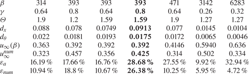
To refine these estimates, we use the numerical results presented in the previous section of the work. Data for some typical parameter values are shown in table 3, where for each simulated case, the numerical values of the damping coefficients  $d_x, d_\theta$, the numerical and theoretical values of the cruising speed coefficient
 $u_\infty ^{num}, u_\infty (\beta )$, the numerical and theoretical estimates of the efficiency
 $\varepsilon _ {num}, \varepsilon _{a}$, are presented.
Analytical and numerical estimates of the key characteristics of the propulsive motion. The column with the parameters of the most efficient motion is marked in bold.

Since the efficiency of movement significantly depends on the cruising speed (as  $u_\infty ^3$), the deviation of this value from the theoretical one most significantly affects the estimates of
 $\varepsilon$. This, in particular, leads to the fact that at high oscillation frequencies, where the cruising speed coefficient (obtained numerically)
 $u_\infty ^{num} < u_\infty (\beta )$ rapidly decreases near the upper boundary of applicability, the theory significantly overestimates the efficiency (see cases
 $\beta = 3142, 6283$). In the range of small amplitudes in the vicinity of the upper limit of applicability, the cruising speed is higher than the theoretical one
 $u_\infty ^{num} \geq u_\infty (\beta )$, which should lead to some increase in efficiency. However, the underestimation of the speed is compensated by the underestimation of the value of
 $d_x$ in the denominator, which is caused by the low accuracy of the approximation of
 $d_x \approx d^{(0)}_x$ at large amplitudes. Therefore, here the theoretical and numerical estimates of
 $\varepsilon _ {num}, \varepsilon _ {a}$ coincide quite well.
The maximum efficiency of motion  $\varepsilon \approx 26\,\%$, achieved at
 $Re \approx 420$ (the corresponding flow regime is shown in figure 8c), is a relatively high score for this range of Reynolds numbers. This result can be compared with the efficiency estimates (calculated in a similar way) of fish-like movement (Maertens et al. Reference Maertens, Triantafyllou and Yue2015) and with the efficiency of various low-Reynolds-number swimmers (Hancock & Newman Reference Hancock and Newman1953; Purcell Reference Purcell1977; Becker, Koehler & Stone Reference Becker, Koehler and Stone2003). The maximum efficiency of the carangiform swimmer at
 $2500 < Re <5000$ is approximately
 $40\,\%$, and of the anguilliform swimmer is approximately
 $30\,\%$. Low-Reynolds-number swimmers have significantly lower efficiency: the Purcell's swimmer has a peak efficiency of
 $0.77\,\%$, the undulating rod is approximately
 $7.4\,\%$ and the helical swimmer is approximately
 $8.6\,\%$. Thus, in terms of relative energy consumption, a cylindrical flapping wing can be attributed to the most efficient propulsors in the range of
 $Re \sim 10^2\text{--} 10^3$.
6. Conclusion
In the work, a propulsive motion of a cylindrical wing of a circular cross-section performing translational–rotational oscillations in a viscous incompressible fluid was considered. To describe the flow past the wing the unsteady Navier–Stokes equation was solved. The solution was constructed as the asymptotic expansion in the small dimensionless oscillation amplitude ( $\gamma \ll 1$). The frequency range was not restricted. The cruising motion regime was investigated, when the average force acting on the body during the period of oscillation is equal to zero. According to the results of the study, the first two terms of the expansion were analytically obtained: the first term describes the primary non-stationary Stokes flow; the second term describes the steady streaming formed as a result of the nonlinear interaction of time harmonics. It was shown that the interaction of time harmonics of translational and rotational oscillations leads to the formation of a non-zero cruising speed of motion.
The cruising speed can be either positive (forward motion) or negative (reverse motion) depending on the dimensionless vibration frequency  $\beta$. The sign change occurs at
 $\beta \approx 13.5355$. In forward motion, the maximum dimensionless cruising speed of the cylinder is
 $3/4 \varTheta$ (three quarters of the maximum angle of rotation), in the opposite direction it is defined as
 $(-0.0534) \varTheta$. For the forward and reverse motion, the analysis of the structure of steady streaming was carried out. Ten main flow regimes A–K are localized by characteristic structural features, a map of regimes in the parametric plane
 $(\beta, \varTheta /\gamma )$ was constructed.
To investigate the limits of applicability of the solution, a series of numerical calculations was performed. A forward regime of motion was simulated in the range of large and moderate values of  $\beta$. Comparison of the results showed that the range of applicability of the constructed asymptotic model (where the difference between theoretical and numerical estimates of cruising speed does not exceed 12 %) for moderate frequencies
 $150 \leq \beta \leq 470$ is defined as
 $0 <\gamma \leq 0.8$,
 $0.3 \leq \varTheta \leq 1.7$, for high frequencies
 $470 <\beta <6500$ is defined as
 $0 <\gamma \leq 0.3$,
 $0.3 \leq \varTheta \leq 1.7$.
Within the framework of numerical modelling, the flow regimes around the cylinder were also analysed. The flow regime D was localized in a significant part of the range of applicability. The numerical results confirmed all the main characteristics of this regime described by the analytical solution: the size and position of the vortices depending on the parameters  $\beta, \varTheta /\gamma$ and its boundary in the parametric plane. We also investigated the flow regimes near the boundaries of the applicability range, where, in particular, the (classical) flows with reverse vortex streets were localized.
Based on the asymptotic and numerical results, the efficiency of movement in terms of energy consumption was estimated. It was found that in the considered range of parameters, the maximum efficiency  $\varepsilon \approx 26\,\%$ is achieved in the region of moderate frequencies
 $\beta \approx 393$ at the highest amplitudes of translational and rotational vibrations
 $\varTheta = 1.59, \gamma = 0.8$. This suggests that, in terms of relative energy consumption, a cylindrical flapping wing can be attributed to the most efficient propulsors in the range of
 $Re \sim 10^2$–
 $10^3$.
The obtained parameters of wing motion are close to the characteristic parameters of the movement of insects. In the optimal regime, at  $\beta \approx 393$,
 $Re \approx 420$, a body with a wing diameter (chord) of 4 mm and an oscillation frequency of 240 Hz, according to the obtained theory, can move in air at an average speed of
 $1.63$ m s
 $^{-1}$. These are the approximate parameters and a flight speed of a housefly (Musca domestica).
Supplementary movies
Supplementary movies are available at https://doi.org/10.1017/jfm.2022.287.
Funding
This paper has been supported by the Kazan Federal University Strategic Academic Leadership Program (“PRIORITY-2030”).
Declaration of interest
The authors report no conflict of interest.
Appendix A. Solution of the secondary flow problem
Let us present more complete formulae for calculation of  $\tilde {\varPsi }_\theta$,
 $\tilde {W}_\theta$ and their derivatives. These decaying exponentially as r goes to infinity functions are solutions of the equations
 \begin{equation} \mathcal{L}_1 \tilde{W}_\theta={-}\beta G_\theta,\quad \mathcal{L}_1 \tilde{\varPsi}_\theta=\tilde{W}_\theta. \end{equation}
To find them we use the method of variation of an arbitrary constant. First, we introduce functions
 \begin{equation} \varphi_1=r^{{-}1},\quad \varphi_2=r,\quad \varphi_3=\tfrac{1}{2}r \ln{r},\quad \varphi_4=\tfrac{1}{8}r^3, \end{equation}
that are fundamental solutions of the equation  $\mathcal {L}_1^2 \varphi =0$:
 \begin{equation} \mathcal{L}_1\varphi_1=0,\quad \mathcal{L}_1\varphi_2=0,\quad \mathcal{L}_1\varphi_3=\varphi_1,\quad \mathcal{L}_1\varphi_4=\varphi_2. \end{equation}
Then we consider the integrals
 \begin{equation} I_k(r)={-}\beta \int_r^\infty \rho \varphi_k(\rho)G_\theta(\rho)\, {\rm d} \rho \quad k=\overline{1,4}. \end{equation}
Carrying out integration by parts in the first two, we obtain
 $$\begin{gather} I_1= \int_r^\infty \varphi_1 \mathcal{L}_1\tilde{W}_\theta\,\rho\, {\rm d} \rho =r\varphi'_1 \tilde{W}_\theta-r\varphi_1 \tilde{W}_\theta'+\int_r^\infty \tilde{W}_\theta \mathcal{L}_1\varphi_1\,\rho\, {\rm d} \rho={-}r^{{-}1}\tilde{W}_\theta-\tilde{W}_\theta', \end{gather}$$
 $$\begin{gather}I_2= \int_r^\infty \varphi_2 \mathcal{L}_1\tilde{W}_\theta\,\rho\, {\rm d} \rho =r\varphi'_2 \tilde{W}_\theta-r\varphi_2 \tilde{W}_\theta'+\int_r^\infty \tilde{W}_\theta \mathcal{L}_1\varphi_2\,\rho\, {\rm d} \rho=r\tilde{W}_\theta-r^2\tilde{W}_\theta'. \end{gather}$$
Expressing  $\tilde {W}_\theta$,
 $\tilde {W}_\theta '$ in terms of
 $I_1$,
 $I_2$ and changing the variable of integration to
 $x = \rho /r$, we find
 \begin{equation} \tilde{W}_\theta ={-}\beta\frac{r^2}{2} \int_1^\infty G_\theta(rx)(x^2-1)\, {{\rm d}\kern0.06em x} ,\quad \tilde{W}_\theta' =\beta \frac{r}{2} \int_1^\infty G_\theta(rx) (x^2+1)\, {{\rm d}\kern0.06em x} . \end{equation}
We carry out similar transformations of the other two integrals
 $$\begin{gather} I_3=r\varphi'_3 \tilde{W}_\theta-r\varphi_3 \tilde{W}_\theta'+\int_r^\infty \overbrace{\tilde{W}_\theta}^{\mathcal{L}_1\tilde{\varPsi}_\theta} \overbrace{\mathcal{L}_1\varphi_3}^{\varphi_1}\,\rho\, {\rm d} \rho= r\varphi'_3 \tilde{W}_\theta-r\varphi_3 \tilde{W}_\theta'+ r\varphi'_1 \tilde{\varPsi}_\theta -r\varphi_1 \tilde{\varPsi}_\theta', \end{gather}$$
 $$\begin{gather}I_4= r\varphi'_4 \tilde{W}_\theta-r\varphi_4 \tilde{W}_\theta'+ r\varphi'_2 \tilde{\varPsi}_\theta-r\varphi_2 \tilde{\varPsi}_\theta'. \end{gather}$$
Expressing  $\tilde {\varPsi }_\theta$,
 $\tilde {\varPsi }_\theta '$ in terms of
 $I_3$,
 $I_4$,
 $\tilde {W}_\theta$,
 $\tilde {W}_\theta '$ and changing the variable of integration to
 $x=\rho /r$, we find
 $$\begin{gather} \tilde{\varPsi}_\theta ={-}\beta\frac{r^4}{16} \int_1^\infty G_\theta(rx)(x^4-4x^2\ln{x}-1)\, {{\rm d}\kern0.06em x}, \end{gather}$$
 $$\begin{gather}\tilde{\varPsi}_\theta' ={-}\beta \frac{r^3}{16} \int_1^\infty G_\theta(rx)( 4x^2(1-\ln{x})-x^4-3)\, {{\rm d}\kern0.06em x}. \end{gather}$$
The contribution to the hydrodynamic force from  $\tilde {W}_\theta$ is calculated according to (2.9a) using (A 7a,b)
 \begin{equation} \langle f_y \rangle = \frac{\xi\gamma}{2\beta}(\tilde{W}_\theta' -\tilde{W}_\theta)_{r=1}=\frac{\xi\gamma}{2} \int_1^\infty G_\theta(x;\beta)x^2\, {{\rm d}\kern0.06em x}. \end{equation}
Its equality to zero is a consequence of the well known formulae for indefinite integrals of cylindrical functions (see Gradshteyn & Ryzhik (Reference Gradshteyn and Ryzhik2007), (5.54) and (5.56)).
Formulae for calculating  $\tilde {\varPsi }_x$,
 $\tilde {W}_x$ and their derivatives are obtained in the same way. These decaying exponentially as r goes to infinity functions are solutions of the equations
 \begin{equation} \mathcal{L}_2 \tilde{W}_x={-}\beta G_x,\quad \mathcal{L}_2 \tilde{\varPsi}_x=\tilde{W}_x. \end{equation}
Here we introduce functions
 \begin{equation} \varphi_1=r^{{-}2},\quad \varphi_2=r^2,\quad \varphi_3={-}\tfrac{1}{4} ,\quad \varphi_4=\tfrac{1}{12}r^4, \end{equation}
that are fundamental solutions of the equation  $\mathcal {L}_2^2 \varphi =0$,
 \begin{equation} \mathcal{L}_2\varphi_1=0,\quad \mathcal{L}_2\varphi_2=0,\quad \mathcal{L}_2\varphi_3=\varphi_1,\quad \mathcal{L}_2\varphi_4=\varphi_2 \end{equation}
and integrals
 \begin{equation} I_k(r)={-}\beta \int_r^\infty \rho \varphi_k(\rho)G_x(\rho)\, {\rm d} \rho \quad k=\overline{1,4}. \end{equation}
Further analysis is completely repeated. Here are the final results
 $$\begin{gather} \tilde{W}_x ={-}\beta\frac{r^2}{4} \int_1^\infty G_x(rx)(x^4-1)\,x^{{-}1} {{\rm d}\kern0.06em x}, \enspace \tilde{W}_x' =\beta\frac{r}{2} \int_1^\infty G_x(rx) (x^4+1)\, x^{{-}1} {{\rm d}\kern0.06em x} , \end{gather}$$
 $$\begin{gather}\tilde{\varPsi}_x ={-}\beta\frac{r^4}{48} \int_1^\infty g(rx)(x^2\,{-}\,1)^3\,x^{{-}1} {{\rm d}\kern0.06em x}, \enspace \tilde{\varPsi}_x' =\beta\frac{r^3}{24} \int_1^\infty G_x(rx) (x^2\,{-}\,1)^2(x^2+2)\, x^{{-}1} {{\rm d}\kern0.06em x} . \end{gather}$$
Appendix B. The structure of secondary flows in limiting cases
B.1. Translational oscillations ( $\xi = 0$)

In the absence of the rotational component of oscillations ( $\xi = 0$), the secondary flows are completely described by the stream function
 \begin{equation} \psi = \gamma{\varPsi}_x (r; \beta) \sin {2\theta}, \end{equation}
that is antisymmetric with respect to  $Ox$ and
 $Oy$ axes. As a result, the flow patterns are the same in each of the four quadrants of the plane.
The presented results (see figure 2) indicate the presence of a critical frequency  $\beta _+ = 37.064$ at which
 ${\varPsi }_x(\infty ) = C_x = 0$. This critical frequency separates the regions of different secondary flow patterns. In the supercritical regime
 $\beta >\beta _+$, the well known ‘cloverleaf’ flow scheme is implemented, when in each of the quadrants there is an RC attached to the cylinder. An oscillating cylinder in this case can be considered as a pump that moves a fluid from the upper (
 ${\rm \pi} /4<\theta <3{\rm \pi} /4$) and lower (
 $-3{\rm \pi} /4<\theta <-{\rm \pi} /4$) regions to the lateral ones (from the north and south to the east and west). At the subcritical case
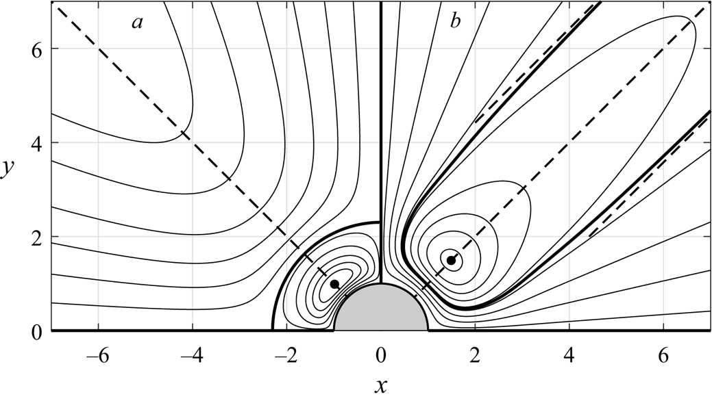
 $\beta <\beta _+$, the RC is not adjacent to the cylinder, but, rather, to the infinitely distant point. The corresponding flow patterns are shown in figure 9.
Streamlines of secondary flows for the case  $\xi = 0$ in (a) supercritical (
 $\beta =70$) and (b) subcritical (
 $\beta =10$) regimes. Bold lines indicate the boundaries of the circulation cells, dotted lines show their asymptotics at
 $r \to \infty$.

B.2. Dominant rotational oscillations ($\xi \to \infty$)

In another limiting case, when  $\xi \to \infty$, the secondary flows are described by a stream function
 \begin{equation} \psi= {\varPsi}_\theta (r;\beta)\cos{\theta}, \end{equation}
that is antisymmetric about the  $Ox$ axis and symmetric about the
 $Oy$ axis. As a consequence, it is sufficient to represent the flow patterns in one of the four quadrants of the plane. The obtained results (see figure 2) indicate the presence of a critical frequency
 $\beta _0 = 13.535$, at which the direction of the motion of the cylinder changes. Another critical frequency
 $\beta _- = 8.35$ is determined by the fact that the function
 $\varPsi (r; \beta _-)$ has a singular point
 $r _- = 3.1$, at which
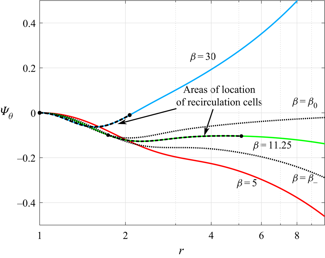
 $\varPsi '(r _-) = \varPsi ''(r _-) = 0$ (see figure 10). At this frequency, the coefficient of cruising speed of the cylinder is
 $u_\infty =-0.0267$. These two critical values of
 $\beta$ separate three possible flow regimes. The first of them, supercritical, is realized for
 $\beta > \beta _0$, and corresponds to the positive direction of motion of the cylinder. It contains no RC in the stream. In the other two regimes, the cylinder moves in the negative direction and the flow contains two RC. In the intermediate regime at
 $\beta _- <\beta <\beta _0$, the cells are located inside the flow region. The corresponding flow patterns are shown in figure 11. The position and size of the RC are shown in figure 10.
Graphs of the function  $\varPsi _\theta (r)$ for different values of
 $\beta$. Dashed lines mark areas of location of RC.

Streamlines of secondary flows for the case  $\xi \to \infty$ in (a) supercritical (
 $\beta = 30$), (b) intermediate (
 $\beta = 11.25$) and (c) subcritical (
 $\beta = 5$) regimes. Bold lines indicate the dividing streamlines.

Let us describe the evolution of RC located at  $\beta _- <\beta <\beta _0$ inside the flow. As
 $\beta$ decreases, the cell decreases in size, degrading at
 $\beta = \beta _-$ to the point with the coordinate
 $r = r_-$ and disappearing when passing through the critical value
 $\beta _-$ to the subcritical flow regime. With an increase of
 $\beta$, the cell, on the contrary, grows indefinitely, approaching the cylinder for
 $\beta \to \beta _0$. At
 $\beta = \beta _+$ the cell becomes infinite and is attached to the cylinder.
B.3. Translational–rotational oscillations of infinitely high frequency ($\beta \to \infty$)

As the dimensionless frequency  $\beta$ tends to infinity, the thickness of the Stokes boundary layers on the cylinder tends to zero. The constants
 $B_x$,
 $B_\theta$ also tend to zero, and
 $C_x$,
 $C_\theta$ take the same value,
 $3/4$. In this case, the stream function, up to an insignificant factor, takes the form
 \begin{equation} \psi=\left(1-\frac{1}{r^2}\right)\sin{2\theta} + \xi \left(r-\frac{1}{r}\right)\cos{\theta}. \end{equation}
Performing an elementary analysis, we find that for  $\xi > 2$ the flow region does not contain RC. For
 $\xi <2$, two symmetric cells are attached to the bottom of the cylinder. Their outer border is an arc of a circle
 \begin{equation} x^2+( y+\xi^{{-}1})^2=\xi^{{-}2}. \end{equation}
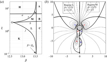
Appendix C. Transitional regimes
The transition between regimes A, B and C of the forward motion and H, K of the reverse motion of the cylinder occurs in a narrow zone near the critical value  $\beta _0$ of the dimensionless frequency. It is shown on in figure 12(a). In this zone three transition regimes can be localized: N is between the main regimes A and H; M is between K and B; L is between K and C. The streamline patterns inside each of the regimes N, M and L are significantly transformed, retaining key characteristics. In the N regime, there are four internal RC and four additional stagnation points (two on the cylinder and two inside the flow). The first pair of cells is located in the upper half-plane and has a characteristic size comparable to the cylinder diameter. The second pair is much larger than the cylinder diameter and is located deep in the lower half-plane. In the L and M regimes there are six cells (two near the cylinder and four inside the flow) and nine additional stagnation points (four on the cylinder and five inside the flow). The difference between these regimes is that in the L regime a special situation is realized when the inner cells are located inside the cells attached to the cylinder. The visualization of these flow regimes is shown in figure 12(b).
Flow regime map in the transition region (a) and streamlines of flows in transitional regimes L and M (b). The designations are the same as in figure 4.

Appendix D. Numerical model
For the numerical solution of the problem of translational–rotational oscillations of a cylindrical wing in a fluid, in this study, the model proposed in the works Nuriev, Egorov & Zaitseva (Reference Nuriev, Egorov and Zaitseva2018); Nuriev et al. (Reference Nuriev, Kamalutdinov and Egorov2019, Reference Nuriev, Egorov and Kamalutdinov2021) was adapted. The plane flow around a cylindrical wing was described by the complete non-stationary system of Navier–Stokes equations. The solution was constructed in physical variables in a Cartesian coordinate system moving translationally with the centre of the cylinder. The secant method was used to determine the cruising speed coefficient  $u_\infty$ of the cylinder motion for the given oscillation parameters
 $(\beta, \gamma, \xi )$. The solution algorithm can be represented as follows.
(1) We chose two initial approximations
$u^0_ \infty$, $u^1_ \infty$ in the vicinity of the cruising speed value obtained in the asymptotic solution. For each of them, the hydrodynamic problem was solved until a periodic steady motion was achieved. The solution was considered steady if the difference in average forces calculated over two consecutive periods did not exceed $\epsilon /100$, where $\epsilon$ is a prespecified small number (in the selected calculation range, it was specified as $\epsilon = 10^{- 5 }$). To reduce the time of solving the hydrodynamic problem in the new approximation $u^{j}_\infty$, the velocity and pressure fields from the old approximation $u^{j-1}_\infty$ were set as the initial solution. The average forces $\langle f_x(u^ 0_\infty ) \rangle, \langle f_x (u^1_\infty ) \rangle$, found in steady-state regimes for corresponding two initial approximations, were used to iteratively refine the solution at the second step.(2) The secant method was used to calculate a new approximation for the speed
$u^j_\infty$ $(j\geq 2)$:
(D 1)For the found value of\begin{equation} u^j_\infty=u^{j-1}_\infty-\frac{u^{j-1}_\infty-u^{j-2}_\infty}{\langle f_x(u^{j-1}_\infty)\rangle - \langle f_x(u^{j-2}_\infty)\rangle}. \end{equation}$u^j_\infty$, by analogy with the first step, the hydrodynamic problem was solved (until the periodic regime was reached) and the average force over the period $\langle f_x(u^j_\infty )\rangle$ was calculated. If the condition $\langle f_x (u^j_\infty ) \rangle <\epsilon$ was satisfied for the found force, then the calculation ended. The resulting solution was accepted as a solution to the original problem. Otherwise, the transition to the beginning of the second step was performed and the next iteration $j = j + 1$ was started.


The simulation of the flow around the cylinder was carried out in a rectangular region of size  $(lx,ly)=(100, 100)$. The size was chosen to minimize the effect of external boundaries on the hydrodynamic forces acting on the cylinder. For discretization of the equations we used the finite volume method. The computation scheme was realized on the basis of the OpenFOAM package (Greenshields Reference Greenshields2019).
The discretization of the computational domain was carried out using block meshes. The resolution near the cylinder was controlled by the linear mesh grading in the direction normal to the boundary of the cylinder. The total number of cells  $N$ for all calculated cases was
 $N\approx 3.8 \times 10^5$.
Discrete values of the velocity components and the pressure were localized in the cell centres of the computational mesh. The Gauss integral theorem was used to calculate the volume integrals over a finite volume. For the approximation of the pressure gradient linear interpolation was used. In the diffusion terms the normal velocity gradients on the cell surface were approximated by a second-order symmetric scheme with correction for non-orthogonality. The implicit Euler scheme was used for the discretization of the time derivative. The time step in all calculations was chosen to satisfy the condition that the minimum number of time steps per period must be at least 4000 (for the accurate resolution of changes of the hydrodynamic force). The discrete problem was solved using a ‘pressure-implicit with splitting of operators’ method (Issa Reference Issa1986; Ferziger & Perić Reference Ferziger and Perić1999). The pressure equation was solved by the conjugate gradient method with a generalized geometric–algebraic multigrid preconditioner. The equations for the velocity components were solved using the biconjugate gradient method with a predictor based on incomplete factorization. Domain decomposition techniques and message passing interface technology were used for the parallelization of the solution algorithm.
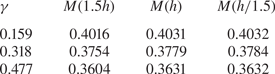
To estimate the accuracy of the calculations, the analysis of the mesh convergence was performed. For this purpose, two auxiliary meshes were constructed in the flow region: the coarse mesh  $M(1.5 h)$, whose cell sizes were increased by 1.5 times (in each direction) compared with the standard mesh
 $M(h)$; and the fine mesh
 $M(h/1.5)$, whose cell sizes were proportionally reduced by 1.5 times. The results of calculation of cruising speed coefficient
 $u_\infty$ on these meshes, presented in table 4, confirm the quadratic character of convergence. Also note that the difference between the results obtained on standard mesh and fine mesh does not exceed 0.15 %.
The values of cruising speed coefficient  $u_\infty$ calculated on different meshes for
 $\beta =393, \varTheta = 1.59$ and various dimensionless amplitudes.