1. Introduction
The green transition is fundamentally transforming economies around the world. The road to environmentally sustainable activities requires unprecedented large-scale investments in technical innovations and renewable energies to reduce global greenhouse gas (GHG) emissions on a path toward net zero (Polzin (Reference Polzin2017), Schnabel (Reference Schnabel2022), Schnabel (Reference Schnabel2023)). Approximately two-thirds of GHG emissions originate from the energy sector (Egli et al., Reference Egli, Steffen and Schmidt2018). Timely investment is critical to limit warming to 1.5 above pre-industrial levels. In line with the Paris Agreement (COP25), the European Union aims for net-zero CO
 $_{2}$
emissions by 2050 to help keep the temperature rise below 2 °C (Boneva et al., Reference Boneva, Ferrucci and Mongelli2021). This would lead to a significant but uncertain increase in risks to the economy and society (Stern (Reference Stern2007), Drudi et al., (Reference Drudi, Moench, Holthausen, Weber, Ferrucci, Setzer, Adao, Dees, Alogoskoufis and Delgado-Téllez2021), Intergovernmental Panel on Climate Change (IPCC) (2018) and Intergovernmental Panel on Climate Change (IPCC) (2021)). Climate change affects the economy through both physical risks (Carney (Reference Carney2015), Alogoskoufis et al., (Reference Alogoskoufis, Carbone, Coussens, Fahr, Giuzio, Kuik, Parisi, Salakhova and Spaggiari2021)) and transition risks (Dennis (Reference Dennis2022), Gourdel et al., (Reference Gourdel, Monasterolo, Dunz, Mazzocchetti and Parisi2024)). The latter arise from potential asymmetric disruptions in typical production costs across sectors.Footnote
1
Production must shift towards greater sustainability, requiring substantial and immediate investments in low-carbon energy, energy efficiency, and possibly CO
 $_{2}$
storage. The relatively high up-front costs of these capital-intensive investments make them particularly vulnerable to changes in the cost of credit (Schnabel, Reference Schnabel2023). In general, all capital investments are affected by credit conditions, but renewable energy assets are especially sensitive (Monnin (Reference Monnin2015) and Fraunhofer Institute for Solar Energy Systems ISE (2024)).Footnote
2
The levelized cost of electricity (LCOE) is a widely used metric in energy investment planning, providing a consistent basis for comparing different methods of electricity generation for a single plant. This statistics measures the average net present cost of electricity generation for a generator over its lifetime (e.g. European Technology and Innovation Platform for Photovoltaics (ETIP PV) (2023) and Dirnbacher (Reference Dirnbacher2024)). Variations in LCOE caused by changes in nominal interest rates affect the cost of energy production through the financing of the up-front cost of the plant and through the discount rate over its lifetime. In periods characterized by relatively low and declining interest rates, the cost of electricity from renewable sources could be considered comparable to that of conventional power plants (Fraunhofer Institute for Solar Energy Systems ISE, 2024). Empirical works confirm that renewable energies become relatively more competitive in such conditions, as their high up-front costs make them far more sensitive to interest rate changes than fossil-fuel plants (Egli et al., (Reference Egli, Steffen and Schmidt2018) and Schmidt et al., (Reference Schmidt, Steffen, Egli, Pahle, Tietjen and Edenhofer2019)). Simulations suggest that the LCOE of a gas-fired power plant would change only marginally if interest rates were to double, while in comparison, offshore wind and solar energy’s LCOE could rise by nearly 45% (International Energy Agency (IEA) and OECD Nuclear Energy Agency (NEA), (2020).Footnote 3
The challenge emerges when changing credit conditions and green investments intersect with climate change.Footnote 4 First, climate change affects inflation through the so-called Climateflation—the impact of extreme weather events such as wildfires, floods, and heatwaves on businesses’ and households’ assets, including warehouses, manufacturing plants, and data centers. These physical risks can reduce production capacity and disrupt supply chains, leading to higher production costs and inflationary pressuresFootnote 5 (Economides and Xepapadeas (Reference Economides and Xepapadeas2018), Alogoskoufis et al., (Reference Alogoskoufis, Carbone, Coussens, Fahr, Giuzio, Kuik, Parisi, Salakhova and Spaggiari2021), Kotz et al., (Reference Kotz, Kuik, Lis and Nickel2024a)). The price effects of physical risk are particularly strong for food prices during heatwaves, and less pronounced during droughts or windstorms.Footnote 6
Second, Greenflation refers to transition risks that include all the costs associated with shifting towards a low-carbon economy (Weber et al., Reference Weber, Thie, Jauregui and Teixeira2024). Greener technologies require significantly larger quantities of minerals (Schnabel, Reference Schnabel2022), which are scarce (Giraud and Valcke, Reference Giraud and Valcke2023) and dependent on uncertain mining discoveries. Global demand for these mineral-intensive technologies can strain production, creating supply bottlenecks and putting upward pressure on pricesFootnote 7
Climateflation and Greenflation influence Central Bank (CB) policy and expose a key dilemma On one hand, the CB can adhere strictly to its traditional inflation-targeting framework, risking a slowdown in green investment and decarbonization. On the other hand, it can include Climateflation and Greenflation into its strategy to support the green transition, though this may partly conflict with its mandate to maintain price stability.Footnote 8
This paper develops a non-linear dynamic model to examine the interaction between monetary policy, Climateflation and Greenflation.Footnote 9 Monetary policy is modeled conventionally, with the CB following a Taylor rule and responding more than proportionally to deviations of inflation from target. The model incorporates a hybrid New Keynesian Phillips Curve inspired by Galı and Gertler (Reference Galı and Gertler1999), where inflation depends on both past inflation and inflation expectations.Footnote 10 We capture the evolution of three key elements: the share of green firms using renewable energy (e.g., solar or wind), the flow of pollution, and inflation expectations. First, the share of green firms follows an exponential replicator dynamics—it evolves path-dependently, based on differences in efficiency between green and brown energy production. For instance, if green energy is less efficient (i.e., has a higher LCOE), the share of green firms declines as firms shift towards brown energy. Second, a higher share of green firms reduces the pollution flow.Footnote 11 Third, inflation expectations are influenced by two factors: the level of pollution, reflecting the effects of Climateflation; and the gap between the share of firms adopting green technology and its available supply, capturing the effects of Greenflation. High demand for green technologies, combined with short-term supply constraints,Footnote 12 can push prices upward.
We obtain a two-dimensional non-linear discrete-time system describing the dynamics of the share of green firms and inflation. We analyze the system’s equilibria and their stability conditions. The most relevant equilibrium is the interior one, where inflation behaves in a standard way - determined by the equilibrium interest rate and the Taylor rule parameters. However, the nominal interest rate also depends on the cost efficiency parameters of the two energy production technologies. Additionally, the share of green firms is influenced by equilibrium inflation as well as parameters related to Climateflation, Greenflation, and the pollution equation. This model allows us to compare the two channels through which climate change affects inflation, within an otherwise standard monetary policy framework. We carefully discuss the parameter choices to assess the magnitude of these effects. We simulate the model under several interesting scenarios: (i) a declining trend in fixed costs, larger for green energy than for brown; (ii) a gradual increase in the short-term fixed supply; (iii) random shocks to the inflation rate; (iv) random shocks to inflation expectations; (v) a one-time positive shock in the inflation target; (vi) a one-time negative shock in the inflation target. These simulations help estimate the timing of the green transition and the short- and long-run dynamics. In summary, the monetary policy trade-off between inflation and green investment remains stable in the third and fourth scenarios, improves in the first, second, and fifth, and worsens in the sixth. Our model also examines the impact of climate change on the natural interest rate through two specific simulations. The overall effect is ambiguous: according to the precautionary savings motive, climate change lowers the natural rate, while increased investment demand and productivity growth push it upward (Drudi et al., Reference Drudi, Moench, Holthausen, Weber, Ferrucci, Setzer, Adao, Dees, Alogoskoufis and Delgado-Téllez2021). Depending on the net result, the likelihood of hitting the Effective Lower Bound could either increase (with a lower natural rate) or decrease.
This paper is innovative for two reasons. First, it directly links Climateflation and Greenflation to inflation expectations and, consequently, to monetary policy decisions, introducing a new source of trade-off for CBs. Second, it models these effects by connecting them to the adoption of green technologies, which depends on differences in energy production efficiency. Related contributions are Chen and Lin (Reference Chen and Lin2024), who use a structural monetary policy VAR and show that monetary tightening reduces renewable energy production (especially solar); Tufail et al., (Reference Tufail, Alvi, Hoang and Wilson2024), who demonstrate that conventional monetary easing in the US, EU, and China positively influences global green investment in both the short and long run; and Jawadi et al., (Reference Jawadi, Rozin and Cheffou2024), who propose a “green” Taylor rule. This paper focuses specifically on potential supply-side challenges that climate change may pose for CB policy frameworks. We do not consider other monetary policy implications of climate change, such as disruptions to the financial system.Footnote 13 To isolate the interaction between climate change and monetary policy, we assume fiscal policy does not play an active role in addressing climate change. Additionally, we exclude carbon pricing and other broad-based climate policies. Evidence suggests these measures tend to be deflationary, as they generate both negative supply and demand shocks (Ferrari and Nispi Landi, Reference Ferrari and Nispi Landi2024). This deflationary effect would counteract the inflationary pressures considered in this paper, thereby mitigating the trade-off between inflation and green investment.
The article is structured as follows. The next section presents the non-linear dynamic model to study the interplay between monetary policy, the evolution of green investment in an industry, and inflation dynamics under Climateflation and Greenflation effects. Section 3 analyses the equilibria and stability conditions. Section 4 discusses model calibration based on existing literature. Section 5 presents the simulation results and Section 6 concludes.
2. The model
To measure the competitiveness or efficiency of an energy-generator technology, we refer to the LCOE indicator. LCOE represents the average revenue per unit of electricity generated that would be required to recover the costs of building and operating a generating plant during an assumed financial life and duty cycle
 $T$
. It is the most common indicator in the literature to evaluate the costs of generating electricity from different sources (coal, natural gas, solar, wind, biomass, etc). It is calculated, in eq. (1), as the ratio between all the discounted expected costs over the lifetime
 $T$
of an electricity-generating plant divided by the discounted sum of the expected energy amounts delivered (Lai and McCulloch, Reference Lai and McCulloch2017).
 \begin{equation} LCOE = \frac {I + \sum _{t=1}^{T} \frac {M_t}{(1+i_t)^t}} {\sum _{t=1}^{T} \frac {E_t}{(1+i_t)^t}} \end{equation}
 $I$
is the initial investment expenditure for the energy plant in the present period
 $t = 0$
, also defined as CAPital EXenditures (CAPEX).
 $M_t$
represents the expected costs of operations, maintenance and fuel in each period
 $t$
over the technology lifetime
 $T$
, also defined as OPerating EXpenditures (OPEX).
 $E_t$
is the electrical energy generated in each period
 $t$
over
 $T$
. Lastly,
 $i_t$
is the interest rate prevailing in the economy in each period
 $t$
that acts as a discount rate in a compound interest rate regime.
2.1. The evolutionary firms’ technological choices
For the sake of simplicity, we focus on an industry composed of
 $n$
homogeneous firms where two different technologies are available: a green/renewable energy generator (
 $G$
) and a brown/fossil-fuel-based energy generator (
 $B$
). To make a fair comparison, the total lifetime of the two investment project options is considered to be the same. We assume each period of time to be a quarter; thus, if we consider a realistic expected financial life of the plants of e.g. 25 years,
 $T = 100$
.
To make analytically treatable the LCOE formula in (1), we assume only two periods of time: present and future. Each firm evaluates the initial investment expenditure
 $I$
at present time
 $t = 0$
, whereas the electricity generated and the operations, maintenance, and fuel expected expenditures will be sustained at a unique point in the future that should well approximate the range of the expected lifetime of the power plant, e.g. from
 $t = 1$
to
 $T = 100$
. To perform this, we employ the concept of the Average Time to Maturity (ATM), which is applicable when the sum of OPEX payments
 $M_t$
and electricity produced
 $E_t$
is expected to be fairly uniform over all quarters
 $t$
of the project duration.Footnote
14
ATM is defined by the parameter
 $m \gt 0$
, which, in our case, given
 $T = 100$
, is equal to
 $m = 50$
. Consequently, it is possible to aggregate all expected OPEX of the green or brown energy plant,
 $j = G, B$
, in a unique parameter
 $M_j$
and discount this value for
 $i_t$
with a simple interest rate regime in eqs. (2) and (3). The same applies to the expected sum of electricity
 $E_j$
generated over the system’s operational life.
LCOE is a “cost” indicator; the lower its value, the better the average cost per energy unit of the plant. The simplified version in eqs. (2) and (3) measure the expected average net present cost of the initial capital and OPEX expenditures over the expected electricity produced during the plant’s lifetime. The levelized cost of electricity indicator for the green/renewable technology is:
 \begin{equation} LCOE_{G,t} = \frac {I_G + \frac {M_G}{1+i_t m}} {\frac {E_G}{1+i_t m}} \end{equation}
The levelized cost of electricity indicator for the alternative brown/fossil-fuel-based technology is:
 \begin{equation} LCOE_{B,t} = \frac {I_B + \frac {M_B}{1+i_t m}} {\frac {E_B}{1+i_t m}} \end{equation}
As pointed out in Section 1, the adoption of renewable energy-based processes requires significant up-front investments. Consequently, we expect the green technology to have a higher CAPEX cost than the brown one, i.e.,
 $I_G \gt I_B$
. However, once established, renewable plants (e.g. solar photovoltaic, biomass, and wind energy) offer an advantage over fossil-fuel-based generators due to the lower cost of maintenance and no fuel expenditure required for energy production (for further details, see the Calibration Section 4). Thus, OPEX are relatively lower for sustainable energy generators:
 $M_G \lt M_B$
. Given the cost structure of the two alternative technologies, the interest rate
 $i_t$
plays a key role in discriminating which investment project, characterized by the same financial duration, is less expensive for the firm in every quarter
 $t$
.
For the monetary policy framework, we introduce a simple Taylor rule that links the quarterly nominal interest rate controlled by the CB
 $i_t$
with the actual inflation rate
 $\pi _t$
:
 \begin{equation} i_t = \bar {i} + \beta \: (\pi _t - \bar {\pi }) \end{equation}
where
 $\bar {\pi }$
is the quarterly inflation target of the CB,
 $\bar {i}$
is the quarterly nominal interest rate target of the CB, and
 $\beta \gt 0$
is the parameter that regulates the sensitivity of the interest rate changes to the actual inflation gap.Footnote
15
It follows that the inflation rate has an indirect effect on the investment projects’ convenience through the monetary policy instrument, i.e., substituting eq. (4) in eqs. (2), (3).
Given the industry of fixed dimension
 $n$
, we introduce a dynamic adjustment to study the evolution of firms’ green and brown investments over time. The dynamic variable
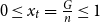 $0 \leq x_t = \frac {G}{n} \leq 1$
represents the share of green investment (i.e., renewable electric generator) employed in the industry in quarter
 $t$
. The complementary dynamic variable
 $0 \leq 1-x_t = \frac {B}{n} \leq 1$
represents the share of brown investment (fossil-based electric generator) employed in the industry in quarter
 $t$
.
The decision of the firms in the industry to invest in the green technology
 $x_t \in [0, 1]$
is assumed to evolve in discrete time, according to an exponential Replicator Dynamics (RD) as in Cabrales and Sobel (Reference Cabrales and Sobel1992):
 \begin{equation} x_{t+1} = (1 -\alpha ) \: x_t + \alpha \frac {x_t}{x_t + (1 - x_t) \: e^{\: \tau (LCOE_{G,t} - LCOE_{B,t})}} \end{equation}
with
 $0 \leq \alpha \leq 1$
and
 $\tau \gt 0$
.
The RD in eq. (5) provides an evolutionary mechanism such that the share of green technology adoption in the industry
 $x_t$
, in the next quarter
 $t+1$
, increases (decreases) when its expected levelized cost
 $LCOE_G$
is lower (higher) than the expected levelized cost of the brown investment
 $LCOE_B$
. The parameter
 $\alpha$
is a proxy of the speed of adjustment in time of the share
 $x(t)$
. A smaller value of
 $\alpha$
signifies greater inertia, reflecting the influence of firms’ switching costs when transitioning from one technology to another. Furthermore, the parameter
 $\tau \gt 0$
measures the firms’ sensitivity to the expected LCOE differential in the technologies available in the industry.
Based on the shares of firms that adopt either the green or brown technology at time
 $t$
, the industry’s level of carbon emissions
 $P_t$
can be identified.
 $P_t$
, expressed in tons of CO
 $_{2}$
per quarter, is a weighted average of the pollution intensity of green generators
 $P_G$
and brown generators
 $P_B$
, with
 $P_B \gt P_G \geq 0$
(see Section 4 for calibration details):
 \begin{equation*} P_t = x_t P_G + (1 - x_t) P_B \end{equation*}
Defining
 $\lambda \equiv P_B - P_G \gt 0$
as the marginal contribution of brown generators to pollution, the expression can be rewritten as:
 \begin{equation} P_t = P_G + \lambda \: (1 - x_t) \end{equation}
2.2. The inflation dynamics
The inflation dynamics is inspired by Galı and Gertler (Reference Galı and Gertler1999) and represented by the following difference equation:
 \begin{equation} \pi _{t+1} = (1-\gamma ) \: \pi _{t} + \gamma \: E(\pi _{t+1}) \end{equation}
Inflation in the next quarter is a weighted average between actual inflation
 $\pi _t$
(i.e., based on the well-known literature on the viscosity of price changes) and inflation expectation
 $E(\pi _{t+1})$
. Agents’ expectations of inflation can have a greater influence on the next quarter’s realization based on the weight
 $0 \leq \gamma \leq 1$
, while
 $1-\gamma$
measures the inertia derived from the actual inflation value. For the equilibrium condition
 $\pi _{t+1} = \pi _t = \pi ^*$
, eq. (7) is a rational expectation equilibriumFootnote
16
(REE) as agents’ inflation expectation coincides with the inflation equilibrium rate:
 $\pi ^{\ast } = E^{\ast }(\pi )$
.
The inflation expectation of agentsFootnote
17
in eq. (8) includes the CB quarterly inflation target
 $\bar {\pi }$
, i.e., the publicly announced CB’s inflation objective around which operators’ expectations are centered, and two expected inflationary effects related to climate change:
 \begin{equation} E(\pi _{t+1}) = \bar {\pi } + \kappa \: P_t + \rho \: (x_t - \bar {x}) \end{equation}
The first expected effect
 $\kappa \: P_t$
is defined in the literature as Climateflation.
Climate change can have significant economic consequences, including damage to infrastructure, disruptions and interruptions of product supply, increased healthcare costs due to climate-related illnesses, and higher insurance premiums for properties exposed to climate risks. These impacts can lead to increased production costs, reduced productivity, and supply chain disruptions, all of which can contribute to inflationary pressures. This effect is positively associated with the number of polluting companies in the economy, contributing to worsening climate-related disasters. In our framework, pollution is positively dependent on the share of firms adopting fossil-fuel-based generators, as highlighted in eq. (6). The emissions related to adopting the brown technology accelerate the pace and the frequency of natural disasters. This creates supply shocks and bottlenecks that, mediated by the parameter
 $\kappa \gt 0$
, ultimately lead to Climateflation.
The second expected effect
 $\rho \: (x_t - \bar {x})$
is denominated Greenflation.
It refers to the rising prices of goods and services due to the costs associated with transitioning to a more environmentally sustainable economy. In fact, in the short to medium term, the supply of intermediate goods (given the scarcity of resources) is given, as is technology, making it complicated to adjust the supply to a growing demand for green technologies. In addition to the expenses related to the implementation and transition to green technologies, complying with regulations to meet environmental standards and adapting to climate change impacts can be expensive. These forces generate upward pressure on prices captured by the term
 $\rho \: (x_t - \bar {x})$
. When the share of green investment in the industry
 $x_t$
(i.e., the demand) exceeds the supply
 $\bar {x}$
, given by the actual level of technology and the number of raw materials and commodities employed in the transition, inflationary pressure mounts mediated by the parameter
 $\rho \gt 0$
.Footnote
18
Changing the fixed supply
 $\bar {x}$
Footnote
19
allows us to consider technological advancements that reduce the shortages or make it possible to assume different supply constraints depending on the specific industrial sector considered.
The result is that Climateflation and Greenflation relate to green firms in an opposite way. The first positively depends on
 $1-x_t$
through the emission generated by this typology of investment, while the second positively depends on
 $x_t$
due to the transition cost associated with the sustainable transition. Generally, the literature distinguishes based on the time horizon of these two effects, identifying the first as a long-run effect on inflation and the second as a short-medium consequence as the economy adjusts to new production and consumption patterns.
In this framework, the CB internalizes the inflation expectation in its monetary policy rule in eq. (4) so that the change of the interest rate instrument could also address the inflation components related to climate change (i.e., dealing with a typical externality) and green transition. In turn, interest rate changes affect the decisions of the firms in the industry because they act as a discount rate in eqs. (2) and (3), changing the cost, measured by the LCOE indicator, of one technology over the other.Footnote 20 All in all, it is possible to close the system by inserting the Taylor rule (4) into the eqs. (2) and (3) and plugging the pollution function (6) in eq. (8).
The resulting two-dimensional non-linear system in discrete time can be concisely represented as the dynamics of the share of firms adopting green technology in the industry and inflation:
 \begin{equation} \begin{cases} x_{t+1} = f (x_{t}, \pi _{t})=(1 -\alpha ) \: x_t + \alpha \dfrac {x_t}{x_t + (1 - x_t) \: e^{\: \tau (LCOE_{G,t} - LCOE_{B,t})}} \\ \pi _{t+1} = g (\pi _{t}, x_{t})= (1-\gamma ) \: \pi _{t} + \gamma \: \left [ \bar {\pi } + \kappa P_{G} + \kappa \lambda \: (1-x_t) + \rho \: (x_t - \bar {x}) \right ] \end{cases} \end{equation}
where
 $LCOE_{G,t}$
and
 $LCOE_{B,t}$
are defined in (2) and (3), respectively, after the insertion of (4).
Since the dynamic adjustment process reported by (9) is expressed in terms of differential equations, the usual methods for analyzing stability, bifurcations and different types of attractors can be applied. This will be the subject of Section 3.
3. Equilibria and stability conditions
To shed light on the dynamic behavior of the system, we will study its equilibrium points, i.e., their position on the phase plane and their local stability. Besides the analytical outcomes, we will also show simulations to provide a graphical visualization of these results in Section 5. Simulations are also useful to study the system’s global properties and stability far from the equilibria. In Section 4, the model will be calibrated using a plausible set of parameters drawn from the empirical literature.
3.1. Boundary equilibria
Map (9) is a two-dimensional discrete-time non-linear dynamical system. The map admits two equilibria that we can label “boundary equilibria” because they are characterized by a share of green investment equal to 0 and 1, respectively:
 \begin{equation} \begin{array} [c]{ccc} E_{0}=\left ( 0, \bar {\pi }+\kappa \left (P_{G}+\lambda \right )-\rho \overline {x} \right ) \,E_{1}=\left ( 1,\bar {\pi }+\kappa P_{G}+\rho \left (1- \overline {x}\right )\right ) \end{array} \end{equation}
We can note that the inflation rate at the equilibrium
 $E_0$
is lower than the inflation rate at the equilibrium
 $E_1$
as long as
 $\rho \gt \kappa \lambda$
.
3.2. Interior equilibrium
Besides boundary equilibria, the map (9) may admit an internal equilibrium (
 $E^*$
), where the share of green investments is neither 0 nor 1. By using the equilibrium condition
 $x_{t+1}=x_{t}=x^{\ast }$
into eq. (5), we find that the interior equilibrium must satisfy the condition:
 \begin{equation*} LCOE_{G}=LCOE_{B} \end{equation*}
which is solved by the following equilibrium value of the nominal interest rate:
 \begin{equation} i^{\ast }=\frac {1}{m}\left [ 1+\frac {E_{G}M_{B}-E_{B}M_{G}}{E_{B}I_{G}-E_{G}I_{B}}\right ] \end{equation}
It follows that the equilibrium value of the nominal interest rate is positively correlated with
 $E_G$
,
 $M_B$
and
 $I_B$
, while it is negatively correlated with
 $E_B$
,
 $I_G$
,
 $M_G$
and
 $m$
.
Given the equilibrium value of the nominal interest rate (11), we can use it into the Taylor rule (4) to get the equilibrium value of the inflation rate:
 \begin{equation} \pi ^{\ast }=\frac {1}{\beta }\left ( i^{\ast }-\overline {i}+\beta \overline {\pi } \right ) \end{equation}
So, the higher is the equilibrium value of the nominal interest rate, the higher is the equilibrium value of the inflation rate. Moreover, while the quarterly inflation target of the CB (
 $\overline {\pi }$
) is positively correlated with the equilibrium value of the inflation rate, the quarterly nominal interest rate target of the CB (
 $\overline {i}$
) is negatively correlated with it. Finally, more complicated is the role of the parameter
 $\beta$
that is positively correlated with
 $\pi ^{\ast }$
if
 $i^{\ast }\lt \overline {i}$
and negatively correlated in the opposite case.
By using the equilibrium condition
 $\pi _{t+1}=\pi _{t}=\pi ^{\ast }$
into eq. (7) combined with eq. (6), we can derive the equilibrium share of green investments:
 \begin{equation} x^{\ast }=\frac {\pi ^{\ast }-\overline {\pi }-\kappa \left ( P_{G}+\lambda \right ) +\rho \overline {x}}{\rho -\kappa \lambda } \end{equation}
to which it corresponds an equilibrium value of pollution:
 \begin{equation} P^{\ast }=P_{G}+\lambda (1-x^{\ast }) \end{equation}
The higher are
 $P_{G}$
and
 $\lambda$
, the lower is the equilibrium share of green investments. It is interesting to look at the relation between inflation rate and share of green investments at the equilibrium. If
 $\rho \gt \kappa \lambda$
they are positively correlated. With feasible values of the parameters (See Table 1 in Section 4), this condition always holds, at least when the equilibrium of the map is the internal one, and not one of the boundary equilibria.
From eq. (7) we also know that at the equilibrium the inflation expectation is equal to the actual value of inflation:
 $E^{\ast }(\pi )=\pi ^{\ast }$
.
3.3 Local stability
In order to study the local stability of the three equilibria, we need to calculate the Jacobian matrix of the dynamical system (9):
 \begin{equation} J:\begin{bmatrix} J_{11} &\quad J_{12}\\ J_{21} &\quad J_{22}\end{bmatrix} \end{equation}
where:
 \begin{equation*} \begin{array} [c]{l} J_{11}=1-\alpha +\alpha \left \{\dfrac {x+(1-x)e^{\tau (LCOE_{G}-LCOE_{B})}-x\left ( 1-e^{\tau (LCOE_{G}-LCOE_{B})}\right ) }{\left [ x+(1-x)e^{\tau (LCOE_{G}-LCOE_{B})}\right ] ^{2}}\right \} \\ \\ J_{12}=\alpha \left \{ \dfrac {-x(1-x)e^{\tau (LCOE_{G}-LCOE_{B})}m\beta \tau \left ( \frac {I_{G}}{E_{G}}-\frac {I_{B}}{E_{B}}\right ) }{\left [ x+(1-x)e^{\tau (LCOE_{G}-LCOE_{B})}\right ] ^{2}}\right \} \\ \\ J_{21}=\gamma ({-}\kappa \lambda +\rho )\\ \\ J_{22}=1-\gamma \end{array} \end{equation*}
The Jacobian matrix (15) must be evaluated at each equilibrium point.
3.3.1. Local stability of
 $E_0$

When we consider the boundary equilibrium
 $E_0$
, we get the following Jacobian:
 \begin{equation*} J_{0}: \begin{bmatrix} 1-\alpha +\dfrac {\alpha }{e^{\tau (LCOE_{G0}-LCOE_{B0})}} &\quad 0\\ \gamma ({-}\kappa \lambda +\rho ) &\quad 1-\gamma \end{bmatrix} \end{equation*}
that is triangular, so it displays the (always real) eigenvalues on the main diagonal:
 \begin{equation*} \begin{array} [c]{lll} \xi _{1}=1-\alpha +\dfrac {\alpha }{e^{\tau (LCOE_{G0}-LCOE_{B0})}}; \,\, \xi _{2}=1-\gamma \end{array} \end{equation*}
Note that
 $LCOE_{G0}$
and
 $LCOE_{B0}$
denote the values of
 $LCOE_{G}$
and
 $LCOE_{B}$
calculated at the equilibrium
 $E_0$
.
While
 $\xi _{2}$
is always positive and lower than one, so it cannot lead to instability, the first eigenvalue
 $\xi _{1}$
may become larger than one for some parameters’ values. In particular the boundary equilibrium
 $E_0$
is locally stable provided that:
 $LCOE_{B0}\lt LCOE_{G0}$
.
3.3.2. Local stability of
$E_1$

Let us consider now the boundary equilibrium
 $E_1$
and the Jacobian matrix (15) calculated at this point:
 \begin{equation*} J_{0}: \begin{bmatrix} 1-\alpha +\alpha e^{\tau (LCOE_{G1}-LCOE_{B1})} &\quad 0\\ \gamma ({-}\kappa \lambda +\rho ) &\quad 1-\gamma \end{bmatrix} \end{equation*}
that is also triangular and the (always real) eigenvalues are:
 \begin{equation*} \begin{array} [c]{lll} \xi _{1}=1-\alpha +\alpha e^{\tau (LCOE_{G1}-LCOE_{B1})}; & & \xi _{2}=1-\gamma \end{array} \end{equation*}
Here
 $LCOE_{G1}$
and
 $LCOE_{B1}$
denote the values of
 $LCOE_{G}$
and
 $LCOE_{B}$
calculated at the equilibrium
 $E_1$
.
Also for
 $E_1$
the eigenvalue
 $\xi _{2}$
does not create stability issues, while the first eigenvalue
 $\xi _{1}$
may become larger than one for some parameters’ values. In particular, the boundary equilibrium
 $E_1$
is locally stable provided that:
 $LCOE_{G1}\lt LCOE_{B1}$
.
3.3.3. Local stability of
$E^*$

It is more complicated to study the local stability properties of the interior equilibrium analytically. Nevertheless, we can say several things using a mix of analytical and numerical tools. First of all by putting the interior equilibrium share of green investment (13) equal to 0, the interior equilibrium value of the inflation rate becomes equal to the one of the boundary equilibrium
 $E_0$
, i.e.,
 $\pi ^{\ast }=\bar {\pi }+\kappa \left (P_{G}+\lambda \right )-\rho \overline {x}$
, while by putting the interior equilibrium share of green investment (13) equal to 1, the interior equilibrium value of the inflation rate becomes equal to the one of the boundary equilibrium
 $E_1$
, i.e.,
 $\pi ^{\ast }=\bar {\pi }+\kappa P_{G}+\rho \left (1- \overline {x}\right )$
.
This means that a transcritical bifurcation occurs involving
 $E_0$
and
 $E^{\ast }$
when the eigenvalue
 $\xi _{1}$
of the Jacobian calculating in the boundary equilibrium
 $E_0$
is equal to 1, that is exactly when the two equilibria are coincident. Similarly, when the eigenvalue
 $\xi _{1}$
of the Jacobian calculating in the boundary equilibrium
 $E_1$
is equal to 1. This is important because at a transcritical bifurcation two equilibria exchange their stability properties, so when
 $E_0$
is unstable, for parameter values close to the bifurcation values,
 $E^{\ast }$
should be stable. Similarly by considering
 $E_1$
and
 $E^{\ast }$
. We must note that the interior equilibrium could also become unstable via a local bifurcation different from the transcritical one (i.e., via period-doubling or Neimark-Sacker bifurcation). Analytical conditions for the occurring of these bifurcations are not easily obtainable. Nevertheless, our numerical simulations show that, for feasible parameters’ values (see Table 1 of Section 4), the only bifurcations we can see are transcritical bifurcations.
A careful calibration is crucial to obtain reliable policy insights from the model dynamics. To this aim, we turn to the existing economic literature to identify meaningful values for the set of parameters of the model in Section 4. In this way, from the multitude of potential scenarios, we can only focus on those that are economically significant for our analysis.
4. Model calibration
We can distinguish between structural parameters and calibrated parameters.
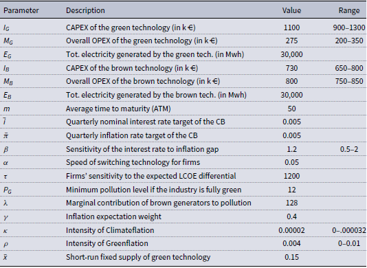
Structural parameters, at the core of the model, include: 1) technology characteristics in terms of costs and energy produced, 2) the monetary policy rule sensitivity to inflation gap, and 3) behavioral factors driving the inflation dynamics, namely the intensity of Climateflation and Greenflation. Calibrated parameters are less central because: 1) they are estimated on the basis of the unit of time considered and only affect the dynamics towards the equilibrium, i.e.,
 $m, \alpha , \tau , \gamma$
, 2) they are linked to hardly changeable characteristics of the industry and/or technology, such as pollution levels and industry’s fixed supply, 3) they are CB inflation and nominal interest rate targets. The first category of parameters can be varied to assess the economic impact on the investment composition of the industry and inflation rates. The second category is assumed to be fixed and calibrated based on the model assumptions. Table 1 provides a summary of the parameters value along with their potential range of variation. As described in the following, these are economically plausible ranges that will be used in the comparative statistic analysis in Appendix A.

The model compares two investment options that, for a fair comparison, have both a lifetime of 100 quarters (25 years).Footnote
21
For the green energy plant, we consider one of the most widespread and well-known renewable technology: an industrial grade solar photovoltaic (PV) investment with a nominal capacity of 1 Mwp.Footnote
22
The global average CAPEX for commercial ground-mount installations between 100 kWp and 2 MWp are estimated to be in a range between 900
 $\unicode {x20AC}$
and 1,300
 $\unicode {x20AC}$
per kilowatt of installed capacity in 2024 (European Technology and Innovation Platform for Photovoltaics (ETIP PV) (2024) and European Technology and Innovation Platform for Photovoltaics (ETIP PV) (2023) for Europe, National Renewable Energy Laboratory (NREL) (2024a) for the U.S., U.K. Department for Energy Security and Net Zero (2023) for UK, Scotland and Ireland, Ricerca sul Sistema Energetico (RSE) (2019) and Lorenzoni and Bano (Reference Lorenzoni and Bano2007) for Italy, Fraunhofer Institute for Solar Energy Systems ISE (2024) for Germany).
The operations and maintenance costs (OPEX) involve ordinary and preventive maintenance, repairing, insurance, regulatory compliance and administrative costs, land and equipment lease, etc. Large-scale solar photovoltaic (PV) technology is among the cheapest power generation technologies for OPEX, at about 11
 $\unicode {x20AC}$
/kWp per year, i.e., for 25 years, 275,000
 $\unicode {x20AC}$
(National Renewable Energy Laboratory (NREL) (2024a) and National Renewable Energy Laboratory (NREL) (2020)). These costs can strongly vary from 20% to 30% of the initial CAPEX whether equipment is rented (e.g. inverter) and/or the PV installation is on a leased land. For this reason, we also assume a sufficiently wide OPEX range between 200,000 and 350,000€. The annual production of a PV depends on its geographical location and panel efficiency. For a temperate continental region, a reasonable value is 1,200 kWh produced per year per KWp of installed capacity (U.S. Environmental Protection Agency (2019) and U.S. Energy Information Administration (2023)). This make the total electricity generated over the plant lifetime equal to around 30,000 Mwh (30,000,000 Kwh).
For the brown technology, to make a simpler comparison, we assume a natural gas-fired combined cycle (CC) power plantFootnote 23 capable of producing the same total level of electricity as the green technology over a 25-year period. The rated capacity of this thermoelectric power plant could be much lower in comparison (for the same amount of energy produced) because the efficiency of the fossil-fuel option is higher than that of most renewable technologies, as it is not tied to solar or wind irradiation. Simple calculations suggest that a 450 kWp natural gas-fired power plant produces the equivalent overall 30,000 Mwh of energy of a 1000 Kwp PV plant.
As of 2024, the capital expenditure (CAPEX) for a modern natural gas CC power plant typically ranges between 1,400
 $\unicode {x20AC}$
to 1,800
 $\unicode {x20AC}$
per kWp of installed capacity. For reference, assuming 1600
 $\unicode {x20AC}$
per KWp provide around 730,000
 $\unicode {x20AC}$
of CAPEX in a possible range of 650,000 – 800,000
 $\unicode {x20AC}$
(National Renewable Energy Laboratory (NREL), 2024b), making it a much cheaper investment than renewable alternatives.
However, the OPEX for this brown technology typically includes fuel costs, labor costs for electricians, mechanics, and technicians required for supervision and routine operations, as well as costs for maintenance, emission compliance, etc. For these reasons, the OPEX of fossil-fuel power plants are significantly higher than the equivalent green alternatives. These costs, net of fuel expenditures, are estimated at about 53
 $\unicode {x20AC}$
/kWp yearly. For the assumed 450 kWp plant, they translate to about 600,000
 $\unicode {x20AC}$
in total (Lo (Reference Lo2014) and National Renewable Energy Laboratory (NREL) (2024b)). In addition, the price of natural gas and, more generally of all energy commodities, has a strong impact on the operating costs of brown technology accounting for up to 40% of total OPEX. It is also quite volatile due to geopolitical factors, transportation costs, and regional availability. It can vary widely between an average value of 10
 $\unicode {x20AC}$
/kWp and 20
 $\unicode {x20AC}$
/kWp per year (Lo (Reference Lo2014) and National Renewable Energy Laboratory (NREL) (2024b)). The recent increase in energy commodity prices due to the COVID-19 pandemic and geopolitical tensions suggests conservatively assuming the natural gas price at 18
 $\unicode {x20AC}$
/kWp, which brings the expense for the entire operation of the fossil-fuel plant to 200,000
 $\unicode {x20AC}$
. This brings the total OPEX of the brown technology to 800,000
 $\unicode {x20AC}$
within a reasonable range of 750,000
 $\unicode {x20AC}$
to 850,000
 $\unicode {x20AC}$
to reflect this possible variability.
Industrial solar panels emit the equivalent of around 41 g of CO
 $_{2}$
per kwh of electricity generated (U.S. Environmental Protection Agency (EPA) (2024), Intergovernmental Panel on Climate Change (IPCC) (2014) and U.S. Environmental Protection Agency (2019)). Most of these lifecycle emissions are tied to the process of manufacturing panels and are offset by clean energy production within the first three years of operation. Over their lifetime, PV emissions are 11–12 times lower than equivalent gas plants (465 g of CO
 $_{2}$
/kWh) and 20 times lower than coal-fired plants (Intergovernmental Panel on Climate Change (IPCC) (2014). On a quarterly basis, this equals to
 $(0.041 \: \text{kg/KWh} \times 1200 \: \text{Kwh}) / 4 = 12 \: \text{kg of CO2}$
for PV and
 $(465 \: \text{kg/KWh} \times 1200 \: \text{Kwh}) / 4 = 140 \: \text{kg of CO2}$
for natural gas-fired technology. In an industry of 1,000 firms, total quarterly emissions range from 12 to 140 tons depending on technology adoption. It follows that, in the pollution eq. (6),
 $P_G = 12$
and
 $\lambda = 128$
, so that
 $P_t$
will be in the calibrated range
 $[12;140]$
.
The parameters
 $m = 50, \alpha = 0.05, \tau = 1200$
are calibrated to reflect plant lifetimes (
 $T = 100$
quarters), and realistic technology adoption rates, considering delays from permitting and inadequate long-term planning. Institutional factors play a critical role in renewable technology adoption, often resulting in insufficient and slow investments in grid infrastructure. This leads to delays in connecting new wind and solar PV plants and limits system flexibility, thereby reducing the cost-effective integration of renewable energy and slowing down the pace of the transition (International Energy Agency (IEA) (2024).
Monetary parameters align with standard assumptions: a 2% for both the annual inflation target and the long-run nominal interest rate target (0.5% quarterly). Inflation expectations weighted at 40% in eq. (7), reflecting gradual inflation adjustment and inertia documented in the literature. Several works (Galı and Gertler (Reference Galı and Gertler1999), Woodford (Reference Woodford2003), Favaretto and Masciandaro (Reference Favaretto and Masciandaro2016), Bacchiocchi and Giombini (Reference Bacchiocchi and Giombini2021)) confirms a non-negligible inflation inertia that often makes shocks not transitory in time (lasting a few quarters), therefore requiring appropriate monetary policy interventions (Clarida et al., Reference Clarida, Galí and Gertler2000). The intensity of such responses, i.e., the parameter
 $\beta$
, depends on the monetary policy stance taken by the CB board, which may also change in the long-run influenced by prevailing views and specific socio-economic situations. Plausible values can range between 0.5 and 2 with the reference set at
 $\beta = 1.2$
(Taylor, Reference Taylor and Taylor1999).
The 2022 heatwave raised European food inflation by 0.43–0.93 points, with projected 2035 warming amplifying this by 30–50% (Kotz et al., Reference Kotz, Kuik, Lis and Nickel2024a). Under projected 2035 temperatures, global headline inflation could rise by 0.32–1.18% annually, with the strongest pressures at low latitudes and during summer months at higher latitudes (Kotz et al., Reference Kotz, Kuik, Lis and Nickel2024a). The model assumes
 $\kappa = 0.0002$
, so that Climateflation effectFootnote
24
is between 0.096% (when industry is fully green) and 1.12% (when industry is fully brown) yearly.
For Greenflation,Footnote
25
we set its intensity to
 $\rho = 0.004$
and a short run fixed supply of green technology at
 $\bar {x} = 0.15$
. Research on Greenflation is limited due to difficulties in isolating it from overall inflation. Most studies use carbon price increases as a proxy. Del Negro et al., (Reference Del Negro, Di Giovanni and Dogra2023) suggest that a carbon tax or strict environmental regulations could raise headline and core inflation by about 2% and 1% within a year, though CB interventions would likely contain further inflation to preserve stability. Similarly, Känzig (Reference Känzig2023) finds that a carbon policy shock in Europe causes a persistent 1% rise in energy prices and a reduction in emissions. The initial share of technology adoption in the industry
 $x_0 \in [0, 1]$
. The minimum Greenflation effect for
 $x_0 = 0$
is:
 $-0.15 \times 0.004 = -0.06\%$
(i.e., −0.24% yearly), while the maximum effect for
 $x_0 = 1$
is:
 $0.85 \times 0.004 = 0.34\%$
(i.e., 1.36% yearly). In other words, the Greenflation effect ranges from –0.24% annually (if green tech demand is below supply
 $x_t \lt \bar {x}$
) to 1.36% annually (if demand exceeds supply
 $x_t \gt \bar {x}$
). However, in the majority of the scenarios,
 $x_t \gt \bar {x}$
and the pressure to go green, given the supply constraint, is reflected in a positive Greenflation effect. We define
 $x_t - \bar {x} \gt 0$
as the shortage share. As increasing firms switch to low-emission technologies (i.e.,
 $x_t$
increases), Greenflation can be expected to exert upward pressure on prices during the transition. The faster and more urgent the shift to a greener economy becomes, the more expensive it may get in the short run.
These parameters underpin the simulations in Section 5, illustrating the system’s dynamics.Footnote 26 Appendix A provides a robustness check, showing how parameter changes affect equilibria using the ranges in Table 1.
5. Simulations and macro dynamics
Starting from the set of parameters identified in Table 1, such that the interior equilibrium exists, we will show the macroeconomic dynamics of the deterministic model in Subsection 5.1 and of some stochastic models (obtained by adding a trend and noise to specific parameters) in Subsection 5.2.
5.1. Deterministic model
The four panels of Figure 1 present the time series of the green technology adopted by the industry
 $x$
(panel a), industry pollution
 $P$
Footnote
27
(panel c) over 120 quarters, and the evolution of inflation rate
 $\pi$
(panel b) and nominal interest rate
 $i$
(panel d) over 40 quarters.Footnote
28
Time series with
 $i.c.$
 $x_0 = 0.15$
for different inflation values.
Note: The time series represent the evolution of the share of green technology adopted by the industry (panel a) and pollution (panel c) over 120 quarters, the dynamics of the inflation (panel b) and nominal interest rate (panel d) over 40 quarters. On the red curve
 $\pi _0 = 0$
, on the blue curve
 $\pi _0 = 0.005$
(
 $2\%$
yearly), on the green curve
 $\pi _0 = 0.01$
(
 $4\%$
yearly). Parameters: Table 1,
 $i.c.$
 $x_0 = 0.15$
.

We show different evolution of the key variables depending on three different initial conditions (
 $i.c.$
) or shocks for the inflation rate (i.e.,
 $\pi _0$
). Figure 1, obtained from the parameters in Table 1, represents an industry characterized by a realisticFootnote
29
initial share of renewable energy generators amounting to
 $x_0 = 0.15$
(15%). The initial quarterly inflation rate in the red curve is very low at
 $\pi _0 = 0$
. On the blue curve,
 $\pi _0 = 0.005$
, corresponding to the annual CB objective of 2%. On the green curve, it is at a considerably higher value of
 $\pi _0 = 0.01$
, meaning a 4% yearly rate.
In the former case, the green transition is more rapid than in the other scenarios, particularly with a sharp increase in renewable technology adoption in the first period. This is benefited by low initial inflation rates and, consequently, interest rates closer to the zero lower bound for the first quarters (i.e., the CB undertakes an expansionary monetary policy). The industry pollution falls down more quickly as more and more firms switch to the less pollutant technology.
Conversely, in the last case, the transition is much slower with even a brief initial phase of increased adoption of the fossil-fuel-based technology. This recall what occurred in the Eurozone following the COVID-19 pandemic, a rapid and sudden spike in energy prices and inflation that slowed down the decarbonization strategy set by the Paris climate goals.Footnote
30
The transition slows as the CB is forced to tackle the positive inflation shock with a restrictive monetary measure: the interest rate remains above the equilibrium for almost ten quarters. This initially hampers the transition with the industry pollution that remains at higher levels for a longer period of time than in the other scenarios, highlighting the monetary policy trade-off at the core of the model. In the event of positive inflationary shocks exceeding the
 $\bar {\pi } = 2\%$
annual target, the CB faces a challenging dilemma: should it prioritize a low and stable inflation environment by raising interest rates, or should it support the green transition by maintaining low interest rates despite elevated inflation?
It is only after 120 quarters (30 years) that all three scenarios converge to the long-run interior equilibrium
 $E^*$
characterized by
 $x^* = 0.4273$
(42.73%),
 $\pi ^* = 0.0078$
(3.12% yearly),
 $i^* = 0.0085$
(3.4% yearly),
 $P^* = 85.3$
. These numerical values of
 $E^*$
can be easily found substituting the set of parameters in Table 1 in equilibrium eqs. (11) - (14). Even though, independently from the initial conditions, the system converges to the same values of
 $E^*$
, the transition to this equilibrium can clearly differs as a result of diverse initial shocks in inflation rates. In all the three scenarios, starting from an initial 15% share of green firms in the industry at
 $t = 0$
results in a yearly Climateflation rate of 0.96%. Following the transition, the green share increases to approximately 43%, leading to a decrease in Climateflation to 0.682%, representing a reduction of −0.278%. Since the actual share or demand of green technology at the beginning of the period equals the fixed supply (i.e.,
 $x_0 = \bar {x} = 0.15$
), Greenflation is zero. However, as the sustainable transition occurs Greenflation steadily increases (as
 $x$
rises in time), until reaching the maximum yearly Greenflation rate 0.4437% after the transition at
 $t = 120$
. The two inflation components move in opposite ways with Climateflation prevailing in the first phase of the transition and Greenflation prevailing in the final period. This is in line with the view of the European Central Bank and Schnabel (Reference Schnabel2022) important speech, where one passage reads: ‘So far, Greenflation has had a much smaller impact on final consumer prices than Climateflation. It is therefore misleading to claim that the greening of our economies is responsible for the painful increase in energy prices. However, as more and more industries switch to low-emission technologies, Greenflation can be expected to put upward pressure on the prices of a wide range of products during the transition period.’
To sum up, for all the above dynamics, the share of firms adopting the renewable technology in the industry increases after the transition, as a result pollution decreases, while the movements of inflation and nominal interest rates depend on the size and sign of the shocks. Shocks in monetary variables are transitory and disappear after a few quarters (e.g. 10 quarters) due to the adjustment of inflation expectations and monetary policy interventions by the CB. However, their effects on real variables persist over time even after several years beyond the period at which interest and inflation rates have reached equilibrium (e.g. 10 vs 120 quarters). The slow pace at which the industry responds to changes in inflation and interest rates is primarily due to the high initial and fixed costs of investing in a particular technology and, more broadly, the legal, technological, and logistical complexities involved in establishing power plants (captured by the parameters
 $\alpha$
and
 $\tau$
). This means that even a relatively small inflationary shock can have a prolonged impact on the transition process. Projection estimates that global renewable capacity is expected to grow by 2.7 times by 2030, driven by climate and energy security policies implemented in nearly 140 countries (International Energy Agency (IEA) (2024). These policies have been instrumental in making renewable energy cost-competitive with fossil-fuel power plants. The European Union and the United States are both forecast to double the pace of renewable capacity growth between 2024 and 2030,Footnote
31
reaching a level of 25% of overall electricity generation.Footnote
32
This is very similar to the share of firms adopting green technology after 24 quarters in the average scenario (
 $\pi _0 = 0.005$
, 2% yearly) represented by the blue curve of Figure 1.
5.2. Stochastic models
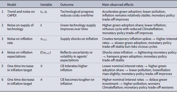
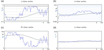
In this section, we analyze the model dynamics under different scenarios (see Table 2 for a summary). For all the simulations, we show the main parameters’ change over the time span and the time series of the green share of firms (
 $x$
), inflation (
 $\pi$
), pollution (
 $P$
) and nominal interest rates (
 $i$
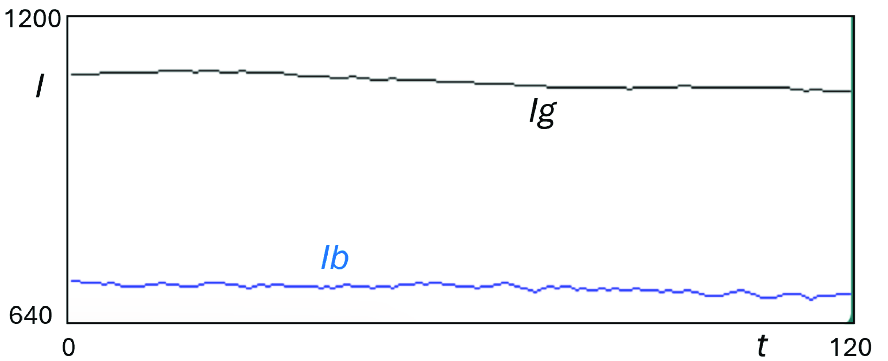
). The time series are shown for 120 quarters as in the deterministic model. In our first stochastic model we endogenize the CAPEX costs as follows:
Summary of the six stochastic models

 \begin{equation*} \begin{array} [c]{l} I_{G,t+1}=I_{G,t}\cdot tr_{G}+\xi _{I_{G}}\\ I_{B,t+1}=I_{B,t}\cdot tr_{B}+\xi _{I_{B}} \end{array} \end{equation*}
where
 $tr_{G}$
and
 $tr_{B}$
can be considered trend component and
 $\xi _{I_{G}}$
and
 $\xi _{I_{B}}$
are additive random noise terms. By interpreting the two CAPEX costs as updating parameters instead of new dynamic variables, we need to update, at each time period, also the equilibrium values of the endogenous variables accordingly.Footnote
33
In particular, we entail a relative reduction in green fixed costs over brown fixed costs by assuming a downward trend
 $tr_{G}=0.9998$
lower than the downward trend
 $tr_{B}=0.9999$
. We also assume the both random noise terms are normally distributed with zero mean, while that standard deviation of the noise term
 $\xi _{I_{G}}$
lower than the standard deviation of the noise term
 $\xi _{I_{B}}$
(1 and 2.5, respectively). The scenario is motivated by expected cost savings for green technologies, and the historical presence of higher variability for brown fixed costs.
Negative trend and noise on CAPEX. Parameters: Table 1.

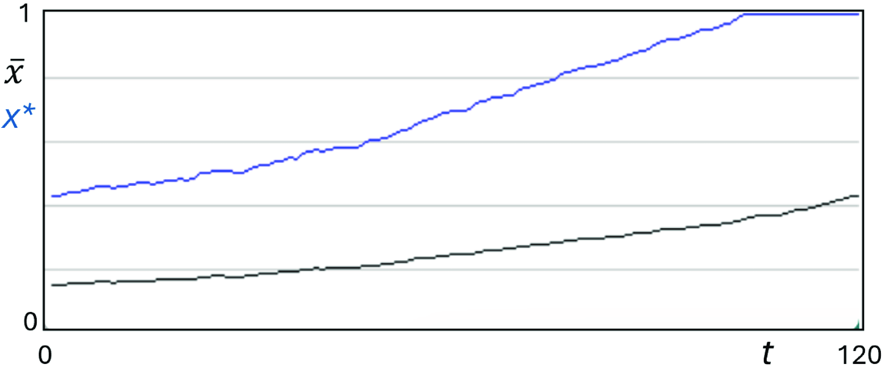
Figure 2 and 3 illustrate actual values (in black) and equilibrium
 $E^*$
values (in blue) for each variable. Actual variables adjust slowly to the equilibrium variables due to the inertia parameters (
 $\gamma$
,
 $\alpha$
). Considering the long-run, the share of green firms is increasing due to the greater trend reduction of the green fixed costs compared to the brown ones (
 $x^* = 0.58$
compared to
 $x^* = 0.43$
of Figure 1). However, CAPEX volatility due to the addition of the random noise leads to short-term variability of the variables. On average, we assist to a larger reduction of the green LCOE vs the brown LCOE that favor the sustainable transition. Pollution, on average, decreases accordingly. Inflation is rather stable after an initial surge due to adjustment toward the equilibrium value. Interest rates show little variations due to the efficacy of their movements in fighting inflation (i.e.,
 $\beta \gt 1$
). There are blue flat areas in the graphs such that the equilibria do not move after reaching one of the two extremes. Those are the equilibrium values where the transcritical bifurcations occur: after reaching the extreme, the interior equilibrium
 $E^*$
is no longer stable while one of the boundary one
 $E_0$
or
 $E_1$
becomes stable. This condition may last until a big enough shock makes the interior equilibrium stable again as it moves away from the extreme. Although the equilibrium value changes in a relevant way, the actual and observable variables (in black) such as the actual firms’ share, inflation rate, etc. moves much more gradually. In general, the simulation shows a negative trend and an additive noise to real variables (the two CAPEX) to reflect the technological advancement in time of the two investment options. Compared to the deterministic model, the trade-off between inflation control and green transition improves when structural costs of green technology decreases more than structural costs of the brown.
Model with negative trend and noise on CAPEX
 $I_G$
and
 $I_B$
.
Note: The time series show the dynamics of green technology share (panel a), inflation (panel b), pollution (panel c), and nominal interest rate (panel d) over 120 quarters. Parameters: Table 1,
 $i.c.$
 $x_0 = 0.15$
,
 $\pi _0 = 0.005$
.

In the second stochastic model we introduce an additive noise term (
 $\xi _{\bar {x}}$
) to the amount of green share of firms that the industry can handle (i.e., in
 $\bar {x}$
) to ensure the avoidance of significant supply-side shortages:
 \begin{equation*} \bar {x}_{t+1}=\bar {x}_{t}+\xi _{\bar {x}} \end{equation*}
In the simulations we consider a normally distributed noise term with positive mean (0.1) to make positive noise more frequent than negative ones. It is not a trend, but in the long run an increasing force on
 $\bar {x}$
should prevail. The standard deviation of the noise term is 0.0002. This implies that the impact on inflation expectations of the Greenflation component is decreasing and may even turn negative (i.e., if
 $x_t - \bar {x} \lt 0$
). The consequence is that as
 $\bar {x}$
increases, the monetary policy trade-off between low inflation and low pollution reduces because the shortage share will become smaller compared to the deterministic model where
 $\bar {x}$
is fixed.
The model is motivated by a growing efficiency in production of green energy technologies that may decrease the bottlenecks due to shortages of rare materials, especially minerals. Economies would eventually learn to decarbonize in a quicker way, hence relaxing the Greenflation constraint and potentially transform it in a positive force for decarbonization (through economies of scale).
Figure 4 and 5 show both actual values (in black) and equilibrium values (in blue) for each variable. Considering the long run, the share of green firms is higher due to the lower shortage share compared to the deterministic model. This causes Greenflation to decrease, or at least not increase, during the transition phase. The reduction in the Greenflation effect increases the long-run share from
 $x^* = 43\%$
of Figure 1 to
 $x^* = 66\%$
, ceteris paribus. This implies lower inflation expectations, hence lower inflation and lower nominal interest rate, that stimulate the adoption of green energy technology. Pollution decreases accordingly and a virtuous cycle starts as Climateflation decreases too. After an initial surge to converge toward the equilibrium value, both actual inflation and equilibrium inflation decrease, improving the monetary trade-off.
There are flat areas in the graphs such that the equilibria do not move after reaching one of the two extremes. Those are the equilibrium values where the transcritical bifurcations occur: after reaching the extreme, the interior equilibrium is no longer stable while the boundary one becomes stable. This happens at the end of the simulation period for
 $x$
and
 $P$
.
Noise on
 $\bar {x}$
. Parameters: Table 1.

Model with noise on supply of technology and materials
 $\bar {x}$
.
Note: The time series show the dynamics of green technology share (panel a), inflation (panel b), pollution (panel c), and nominal interest rate (panel d) over 120 quarters. Parameters: Table 1,
 $i.c.$
 $x_0 = 0.15$
,
 $\pi _0 = 0.005$
.

Our third stochastic model entails an additive random noise on inflation (
 $\xi _{\pi }$
) to capture possible supply-side shocks or other inflationary effects not explicitly considered in our model:
 \begin{equation*} \pi _{t+1}=g(\pi _t,x_t)+\xi _{\pi } \end{equation*}
where
 $g(\pi _t,x_t)$
is the inflation dynamics defined in map (9).
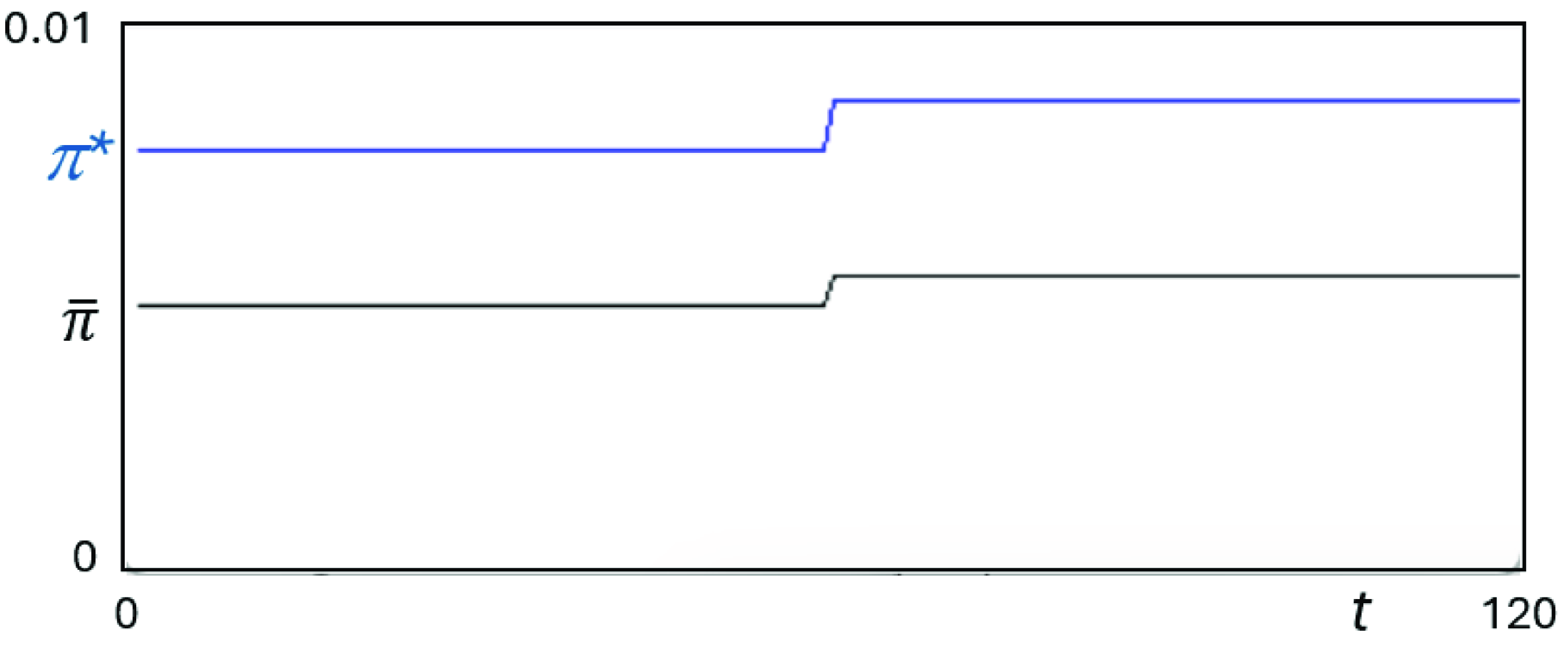
In the simulations, we use a normally distributed random term with zero mean and standard deviation equal to 0.001. Equilibrium values are not affected (they remain the same as the deterministic model of Figure 1) but there is transitory divergence. Indeed, a temporary increase (shock) in inflation spurs an increase in nominal interest rate and thus a decrease in adoption of green energy technologies (i.e., a decrease in
 $x$
). This reduction implies higher pollution levels of the industry, hence higher Climateflation and then inflation, generating a vicious cycle until a big enough countershock hits. The monetary policy trade-off between low inflation and low pollution is stable. The variability of nominal interest rate is higher than the one on inflation due to the efficacy of monetary policy reaction (i.e.,
 $\beta \gt 1$
): deviations of inflation from the target are met by higher deviations of interest rates. Figure 6 shows both actual values (in black) and equilibrium values (in blue) for each variable. The change in the green share and pollution levels of the industry reflects the interest rate movements.
Model with noise on inflation rate
 $\pi _{t+1}$
.
Note: The time series show the dynamics of green technology share (panel a), inflation (panel b), pollution (panel c), and nominal interest rate (panel d) over 120 quarters. Parameters: Table 1,
 $i.c.$
 $x_0 = 0.15$
,
 $\pi _0 = 0.005$
.

Our fourth stochastic model entails an additive random noise on inflation expectations (
 $\xi _{E}$
) to consider the inherent uncertainty of expectations (i.e., it can also be interpreted as the expectation error term):
 \begin{equation*} E(\pi _{t+1}) = \bar {\pi } + \kappa \: P_t + \rho \: (x_t - \bar {x})+\xi _{E} \end{equation*}
In the simulations we use a noise term normally distributed with zero mean and standard deviation equal to 0.001. The overall effect is very similar to the third one. Equilibrium values are not affected but transitory divergences can occur. For example an increase in inflation expectations (shock) positively affects inflation and spurs a tightening in nominal interest rate. The latter leads to a rise in adoption of brown energy technologies. This means higher industry pollution, hence higher Climateflation and inflation, generating a vicious cycle until a big enough countershock hits. Also in the case, the monetary policy trade-off between low inflation and low pollution is stable as equilibrium values are constant. The variability of nominal interest rate is higher than the one on inflation due to the efficacy of monetary policy reaction (i.e.,
 $\beta \gt 1$
): deviations of inflation from the target are met by higher deviations of interest rates.
Figure 7 shows both actual values (in black) and equilibrium values (in blue) for each variable.
Model with noise on inflation expectation
 $E(\pi _{t+1})$
.
Note: The time series show the dynamics of green technology share (panel a), inflation (panel b), pollution (panel c), and nominal interest rate (panel d) over 120 quarters. Parameters: Table 1,
 $i.c.$
 $x_0 = 0.15$
,
 $\pi _0 = 0.005$
.

Our fifth stochastic model entails a one-time positive shock in the inflation target at the 15-year mark (i.e., a one-time increase in
 $\bar {\pi }$
from 0.005 to 0.0055). We interpret this shock on the target level of inflation
 $\bar {\pi }$
as the effect of a permanent increase in past pollution flows that contributes to raising the average level of temperatures and, ultimately, food inflation and headline inflation (Kotz et al., Reference Kotz, Levermann and Wenz2024b). The CB could move toward a more flexible monetary policy framework and reassess its inflation target to better respond to the supply-side shocks that are likely to become more frequent due to climate change (Barmes et al., Reference Barmes, Claeys, Dikau and da Silva2024). In this case, from the 60th semester, the CB inflation target permanently moves from the yearly 2% to a 2.2% (Figure 8). This implies a decrease in the nominal interest rate by the Taylor rule through the inflation gap component
 $\pi _t - \bar {\pi }$
of eq. (4) and an increase in inflation expectations through eq. (8). The overall short-run effect on nominal interest rate is always negative (since
 $\gamma \Delta \bar {\pi }\lt \beta \Delta \bar {\pi }$
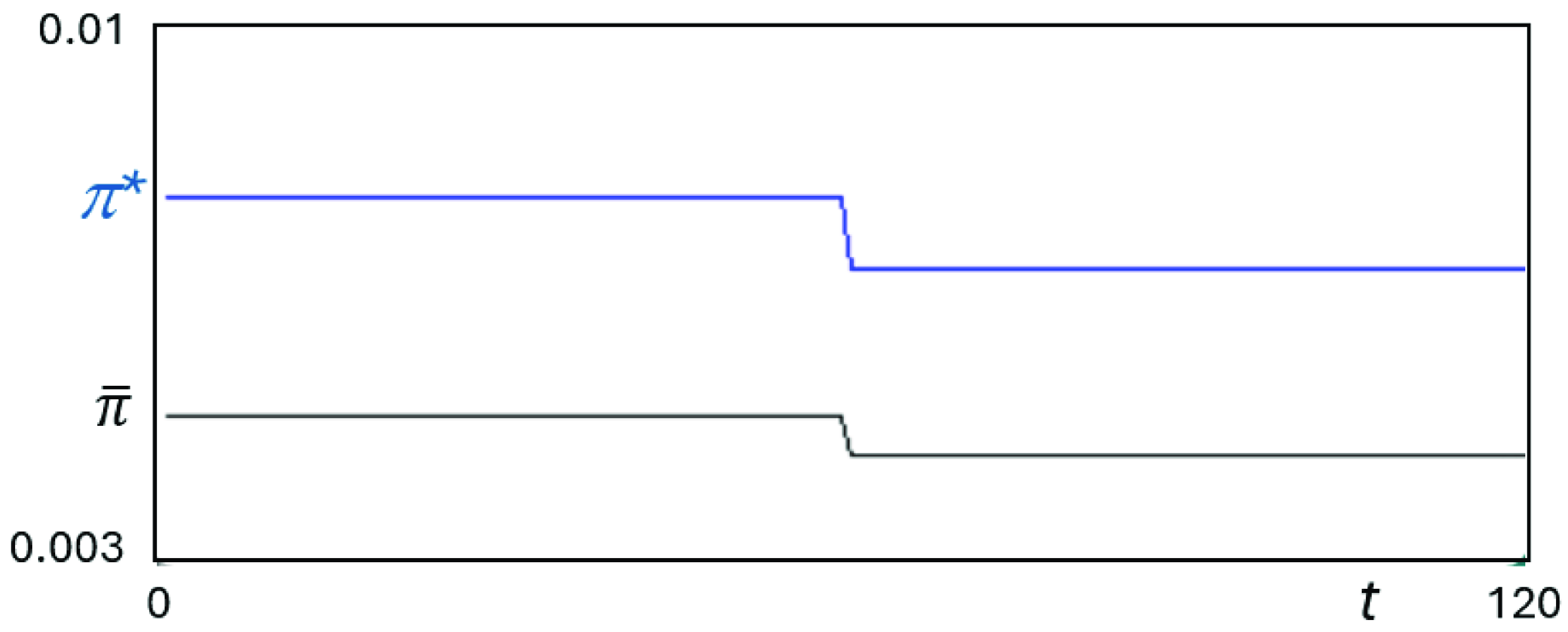
), but then the actual nominal interest rate (in black) slowly increases back to reach its equilibrium value (in blue) at the end of the period. The equilibrium value of the interest rate does not change because it only depends on technological characteristics of the two plants (costs, energy produced and expected lifetime), see eq. (11). Instead, inflation equilibrium is affected. After an initial increase of actual inflation to reach its equilibrium, a second spike at
 $t = 60$
occurs to meet the new higher inflation equilibrium. The effect of a lower actual interest rate (even if only transitory, from
 $t = 60$
to
 $t = 120$
) implies that, in this period, the cost efficiency of the green energy technology increases more than the cost efficiency of the brown technology (i.e.,
 $LCOE_G$
decreases more than
 $LCOE_B$
). This is evident from the vertical increase of equilibrium share
 $x^*$
(in blue) that implies an acceleration in green technology adoption
 $x$
(in black). The share of green firms keeps increasing toward this higher equilibrium, while the pollution decreases more quickly toward the lower equilibrium. Overall, the
 $\bar {\pi }$
one-time increase has a large positive effect on the actual green technology adoption (i.e., at the end of the period
 $x^* = 0.59$
compared with
 $x^* = 0.43$
of Figure 1) and, consequently, a beneficial effect on pollution. This at the expense of a moderate increase in long-run inflation. This happens because, given the parameter set, the monetary policy trade-off between low inflation and low industry pollution slightly improves.
One-time positive shock on
 $\bar {\pi }$
(from 0.005 to 0.0055). Parameters: Table 1.

This scenario can be traced back to the impact of climate change on the natural real interest rate, which can be defined as
 $\bar {r} = \bar {i}-\bar {\pi }$
(Drudi et al., Reference Drudi, Moench, Holthausen, Weber, Ferrucci, Setzer, Adao, Dees, Alogoskoufis and Delgado-Téllez2021). Research shows that the sign of change is uncertain. Lower natural interest rate (shown above) would mean that supply-side effects of climate change are larger than demand side effects: the increase in prices is structural and not counterbalanced by lower demand due to precautionary motives. The opposite would be true in the scenario below.
Model with one-time positive shock in
 $\bar {\pi }$
(from 0.005 to 0.0055).
Note: The time series show the dynamics of green technology share (panel a), inflation (panel b), pollution (panel c), and nominal interest rate (panel d) over 120 quarters. Parameters: Table 1,
 $i.c.$
 $x_0 = 0.15$
,
 $\pi _0 = 0.005$
.

One-time negative shock on
 $\bar {\pi }$
(from 0.005 to 0.0045). Parameters: Table 1.

Our sixth stochastic model entails one-time negative shock in the inflation target at the 15-year mark (i.e., a one-time reduction in
 $\bar {\pi }$
from 0.005 to 0.0045). In this case, from the 60th semester, the CB inflation target permanently moves from the yearly 2% to a 1.8% (Figure 10). It is the symmetric opposite scenario of the fifth model (see Figure 11).
5.3. The effect of climate tipping points
Climate tipping points refer to large-scale discontinuities in the climate system that can trigger abrupt and potentially catastrophic releases of polluting materials, especially CO
 $_{2}$
. Examples include the melting of Arctic or Antarctic ice sheets or the collapse of the North American boreal forest (Lenton et al., Reference Lenton, Rockström, Gaffney, Rahmstorf, Richardson, Steffen and Schellnhuber2019). While some of these events may materialize only in the distant future, others have already been set in motion. Moreover, a growing body of empirical and theoretical research suggests that such tipping points may be reached more rapidly than previously anticipated.Footnote
34
These large-scale shocks may be modeled as temporary increases in the flow of pollution, under the assumption that they do not result in a permanent increase in pollution stock (see Figure 12). If, instead, the tipping event leads to irreversible changes in the climate system, the corresponding shock to pollution flows would also be permanent, thereby generating persistent effects on both climate and economic dynamics (see Figure 13). For the events expected to occur further in the future than the temporary or permanent pollution shocks described above, the most appropriate modeling strategy is to represent them as positive shocks to inflation expectations. This approach is observationally equivalent to a shock to the long-run inflation target
 $\bar {\pi }$
(see Figure 8 and Figure 9).
Model with one-time negative shock in
 $\bar {\pi }$
(from 0.005 to 0.0045).
Note: The time series show the dynamics of green technology share (panel a), inflation (panel b), pollution (panel c), and nominal interest rate (panel d) over 120 quarters. Parameters: Table 1,
 $i.c.$
 $x_0 = 0.15$
,
 $\pi _0 = 0.005$
.

One-time positive shock to
 $P_t$
( +10).
Note: The time series show the dynamics of green technology share (panel a), inflation (panel b), pollution (panel c), and nominal interest rate (panel d) over 120 quarters. Parameters: Table 1,
 $i.c.$
 $x_0 = 0.15$
,
 $\pi _0 = 0.005$
.

Permanent positive shock to
 $P_t$
( +10).
Note: The time series show the dynamics of green technology share (panel a), inflation (panel b), pollution (panel c), and nominal interest rate (panel d) over 120 quarters. Parameters: Table 1,
 $i.c.$
 $x_0 = 0.15$
,
 $\pi _0 = 0.005$
.

6. Conclusion
This paper builds a non-linear discrete-time model to study the interaction between monetary policy and two consequences of climate change, such as climateflation and greenflation. The setup includes a CB following a standard Taylor rule with inflation targeting and a hybrid New Keynesian Phillips curve such that inflation depends on past inflation and inflation expectations. We add a novel monetary policy dilemma arising from the inflation-pollution trade-off via the impact of monetary policy on the relative cost efficiency of energy production technology. This is done by considering the choice of firms between green and brown energy production. This choice affects the overall level of pollution in the economy and its consequences. Indeed, on the one hand, pollution implies climateflation, so the CB implements contractionary monetary policy to reverse it. This leads to lower technology (and higher pollution), hence higher climateflation, creating a vicious circle. On the other hand, an expansionary monetary policy increases green technology adoption (and lower pollution), but implies greenflation because the supply of green technology is fixed in the short run. This creates an incentive for the CB to reverse the expansionary policy in order to return to inflation targeting.
We discuss the equilibria and their stability conditions. The most interesting equilibrium is the interior one. In this equilibrium, inflation is quite standard as it depends on the equilibrium interest rate and the parameters of the Taylor rule. However, the equilibrium interest rate depends on the cost efficiency parameters of the two energy production technologies. In addition, the share of green firms depends on both the equilibrium inflation and the parameters from the climateflation component, the greenflation component and the pollution equation. We carefully calibrate and simulate the model under different scenarios: (i) a trend reduction in fixed costs, which is larger for the green energy than the brown one, (ii) a trend increase in the short-term fixed supply, (iii) a noise on the inflation rate, (iv) a noise on inflation expectations, (v) a one-time positive shock in the inflation target, (vi) a one-time negative shock in the inflation target. These simulations allow us to estimate the timing of the green transition and both the short- and long-run dynamics. Briefly stated, the monetary policy trade-off between inflation and green investment is stable in the third and fourth scenarios, improves in the first, second and fifth, deteriorates in the sixth.
This paper is innovative for two reasons. First, it links directly climateflation and greenflation to inflation expectations and thus to monetary policy decisions, modeling a new source of trade-off for CBs. Second, it models these effects by relating them to the adoption of green technologies based on differential efficiency of energy production.
Further research could explicitly model the relation between stock and flow of pollution, introducing a new dynamical equation to the system, as well as focusing on the potential precautionary savings motive on the demand side (induced by climate change), fiscal policy in the form of incentives for green energy technology, and carbon taxation as a policy tool against climate change.
Competing interests
The authors have no conflicts of interest to declare. All co-authors have seen and agree with the contents of the manuscript and there is no financial interest to report. We certify that the submission is original work and is not under review at any other publication.
A. Appendix. Comparative statics analysis
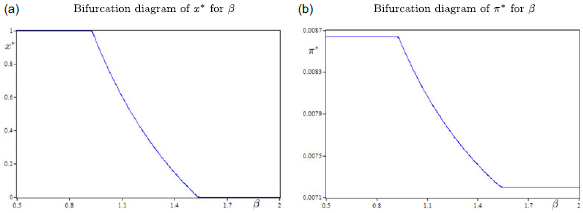
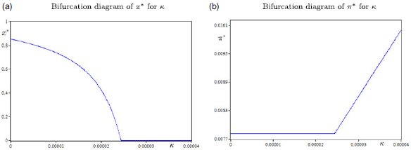
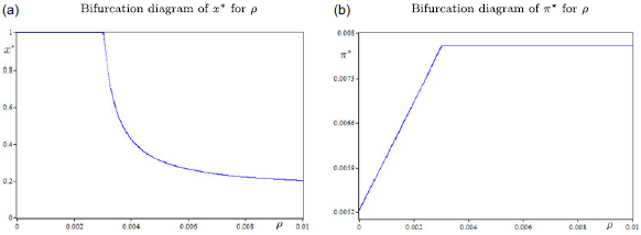
In this section, we let individual parameters vary to perform a comparative analysis on the long-run values at which the system converges. This allows to highlight the parameters thresholds when the transcritical bifurcations occur with the exchange of stability between the boundary equilibria and the interior equilibrium, as demonstrated in Section 3.
In particular, the analysis focuses on structural parameters changes along the range of variation described in Table 1: from the CAPEX and OPEX costs of the two technologies, to the monetary policy response, to the intensity of both Climateflation and Greenflation effects.
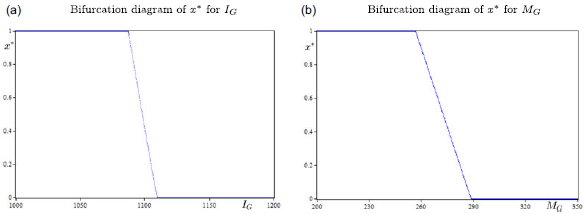
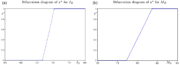
In Figure 14, if both CAPEX and OPEX costs of the renewable energy plant increase, the share of green investment in the industry falls down. The decline of green firms is quick and concentrated in a relatively small range of
 $I_G$
and
 $M_G$
values. This is a consequence of the de facto arbitrage on energy technologies, whereby companies shift (albeit after a long period of time) investments if the relative cost efficiency of green technology is lower than the one for brown technology.
Comparative analysis of green technology costs. Parameters: Table 1.

Comparative analysis of brown technology costs. Parameters: Table 1.

In Figure 15, if both CAPEX and OPEX costs of the fossil-fuel energy plant increase, the share of the alternative green investment in the industry goes up: the increase in green firms share is again swift and concentrated in a relatively small range of
 $I_B$
and
 $M_B$
values. This confirms the strategic relevance of technology cost and the sensitivity of firms to (small) LCOE differential.
In Figure 16, if we increase the response of the CB’s monetary policy to the current inflation gap, it comes a point where the temporary increase in interest rate after a shock is enough strong to make the green energy technology less cost efficient than the brown one, hence all firms choose to implement the brown one (i.e.,
 $x^*=0$
). At the same time, equilibrium inflation decrease accordingly, while equilibrium pollution of the industry is greater: the inflation-pollution trade-off. This, intuitively, means that the CB, if it is tougher at fighting inflation (i.e., greater
 $\beta$
), can reduce long-run inflation, at the expense of a lower share of green investment in equilibrium. On the other hand, if its monetary policy is more accommodating (i.e., lower
 $\beta$
), the sustainable transition will be favored at the cost of higher equilibrium inflation.
In Figure 17, an increase in the Climateflation effect (through an increase in
 $\kappa$
), for the same pollution level the industry generates, leads to greater environmental damage and a rise of inflation in equilibrium. The CB responds, through its Taylor rule, with a restrictive monetary policy. Higher interest rates mean less favorable conditions for green investment (i.e., lower
 $x^*$
).
In Figure 18, an increase in the Greenflation effect (through an increase in
 $\rho$
), for the same scarcity share, increases the equilibrium inflation rate due to the greater prices pressure of the transition. Higher inflation means restrictive monetary policy that favor the green technology, sharply reducing the green firms share in equilibrium. However, as
 $\rho$
increases and
 $x^*$
decreases, reaching the supply constraint threshold
 $\bar {x} = 0.15$
, the pressure on prices stops (for
 $x^* = 0.15$
demand equals supply, the scarcity share is zero, and also Greenflation becomes zero) with equilibrium inflation that from here on remains flat.
Change in monetary policy response. Parameters: Table 1.

Change in the intensity of climateflation. Parameters: Table 1.

Change in the intensity of Greenflation. Parameters: Table 1.