NOMENCLATURE
- API
-
Application programming interface
- BC
-
Boundary Condition
- BIM
-
Building Information Modelling
- CAD
-
Computer-Aided Design
- CAE
-
Computer-Aided Engineering
- CFD
-
Computational Fluid Dynamics
- DND
-
Drag-aNd-Drop
- FEA
-
Finite Element Analysis
- GA
-
General Assembly
- Geom
-
Geometry
- GUI
-
Graphic User Interface
- MCT
-
Mesh Constraint Topology
- LOD
-
Level of detail
- LOA
-
Level of abstraction
- HPC
-
High-pressure Compressor
- VT
-
Virtual Topology
1.0 INTRODUCTION
Thermal-mechanical design is crucial for engine performance analysis because it allows clearances and static deflections in the hot parts to be computed, thereby ensuring that the running configuration of the engine meets its intended performance. It is an iterative process due to the strong coupling between the running configurations and the resulting engine performance. However, performing design iterations between aerodynamic and thermal models for large assemblies is difficult. This is also true even at the engine preliminary design phase, where the most modelling, simulation and analysis tasks can be largely done on reduced models (e.g., from 3D to 2D, and from 2D to 1D or 0D) to cut down the design time and simulation efforts(Reference Robinson, Armstrong and Fairey1-Reference Hun4). The difficulty associated with these iterative design processes is due not only to the presence of a large number of data, but also due to the to-be-solved bottleneck, namely, it is difficult to re-assemble the thermal models with maintained consistency and coherency, during the geometry modification process. Given the initial geometry (Geom.) and thermal Boundary Conditions (BCs) data, the first design cycle produces the first version of the meshing result. Then, the downstream simulation and post-processing process will proceed. This process will reiterate, wherein the post-processing result requests changes towards the geometry will incur further updates to its mesh and simulation results. Within such design workflow, the conventional design tools and design routes failed to convert the geometric model configuration into thermal model BC configuration directly and automatically. In other words, there is a missing link between the geometric and thermal models in the above-mentioned design process, which prevents design automation.
Traditional design processes separate the geometric and physical models (e.g., thermal models). The geometric models are solely made up of groups of geometric primitives, such as points, lines and surfaces, to represent the structure of the engine(Reference Srinivas and Shapiro5-Reference Hoffmann and Juan8). These entities contain neither functional information nor explicit information about design intents. The emergence of feature-based geometrical modelling, on the other hand, enables more physical information and design intent to be carried by the geometric models(Reference Shah and Martti9-Reference Rafael, Eastman and Lee14). However, there is no strict definition of the concept of feature for various feature-based Computer-Aided-Design (CAD) products. A general definition may be drawn from the previous literatures (e.g., Shah and Martti(Reference Shah and Martti9), Hoffman and Hoffman and Joan-Arinyo(Reference Hoffmann and Joan-Arinyo15), Bronsvoort et al(Reference Bronsvoort, Bidarra and Nyirenda12) and Rezayat(Reference Rezayat16)). A feature is generally defined as a region of a part or an assembly mappable to a generic shape which is associated with functional engineering significance. The extra information layer attached to the geometry may include the component semantics, material information, and so on. Regarding gas turbine designs, the information can be of the data pertaining to the aero-thermal performance carried by a component. In this article, we define the feature as an abstract engine assembly entity, which can be associated with geometry and physical data when necessary. This is different from some major CAD systems, wherein features can be recognised as anything, ranging from low-level geometric primitives (e.g., points, lines, fillets) or geometric operation instructions (e.g., extrude or revolve) to geometrically bounded and connected parts and assemblies (e.g., boss and holes).
Using features to carry additional information other than just the geometry per se – e.g., BC data – for engine analysis, is a promising solution to bridge the gap between the geometric and the physical models. This concept is widely applicable to various engineering design sectors, such as civil building construction( Reference Rafael, Eastman and Lee 14 , Reference Ghang, Sacks and Eastman 17 , Reference Cavieres, Russell and Tristan 18 ). For example, the knowledge-based Building Information Modelling (BIM) system proposed by Rafael et al(Reference Rafael, Eastman and Lee14) enabled users to embed design knowledge into a parametric CAD system through features which achieved a fast redesign process by sharing and reusing existing designs. In the aerospace and automotive industry, the concept of “associative geometry”, in which attribute systems (e.g., Feature BCs) are embedded within the geometric model, has been extensively used for some years. For example, the CAD/CAE modeling tool Patran was using associative geometry in the 1990s(Reference Roehl19). Similarly, Abaqus was built around the concept of attaching BCs to geometric model entities. Many of these systems are now fully integrated into the larger CAD systems like CATIA and Siemens NX, both of which are well received in the aerospace industry. These feature-based CAD design tools, to a large degree, indeed alleviated the mismatch between geometric models and simulation models. However, they tend to tackle the problem through lower-level feature primitives e.g., associate the BCs to the edges. One of the shortcomings associated with such approach is that it is ineffective to handle topological changes. For example, assembly fidelity alterations (e.g., adding/removing a feature to/from a part assembly) are likely to result in a disordering of the BCs, or the breaking of the link between the CAD model and the mesh(Reference Foucaulta, Cuillirea, Franoisa and Maranzanac20). Also, the assignments of the BCs to the feature objects, such as finding the insertion position on an edge, are mainly achieved through manual labour and can be cumbersome. Further, the capabilities demonstrated in these commercial software packages are not generic, thus difficult to interface with other simulation tools. For example, some structural analysis tools (e.g., the SC03 proprietary FEA software in a major aero-engine company) require a separate BCs definition file in a specific data format along with its geometric definitions for meshing and analysis, whereas converting data to such formats through the existing CAD tools can be non-trivial. Therefore, a more generic strategy is desired to attach the correct BCs to the feature entities intelligently and effectively.
Some research endeavours have been exerted in the last decades trying to combine the CAD model with the downstream CAE models. These efforts include introducing a common master data structure to contain both geometric and simulation data (such as Lee's CAD-CAE integration approach(Reference Hun4)) and creating an intermediate STEP file to host both the geometric model and additional design intent information(Reference Pratt, Bill and Ranger21,Reference Kim22) . However, apart from the inherent disadvantage these approaches suffered, namely the inevitable need for extra data structure layers prior to the design and meshing, how these reported systems deal with topological changes at engine system level was not clear. In addition, how the adjustments of BC data and constraints are made according to the undertaken geometric transforms were not mentioned. Another attractive solution to address the missing link between the geometry and its simulation models is through the Virtual Topology (VT) technology(Reference Sheffer23,Reference Sheffer24) . This concept has then been significantly developed and advanced by Armstrong et al(Reference Robinson, Armstrong and Fairey1,Reference Nolan25-Reference Tierney27) . The idea of VT is to keep a virtual analysis model topology (the fidelity of which can vary during the design course) along with, but independent from, the actual geometry topology itself. Accompanied by the other two enabling techniques, i.e., Cellular Modelling and Equivalencing, the CAD model is able to undergo arbitrary fidelity changes (through partitioning and merge) to generate various analysis representations, while still maintaining their relationships (through Equivalencing) as per the base geometry throughout the design pathway. The data structure used by Armstrong et al is able to couple with physical models, analysis types and decisions, BCs and other analysis information. These are referred as “simulation intent” to guide the system's automation at the simulation phase. The VT concept, in a way, is similar to the feature-tree concept described in this article. Connected in a tree-like data structure, it can undergo topology changes quickly to adopt fidelity changes, with some degrees of automation, to fit a specific analysis purpose; and at the same time, maintains the consistency and coherency between the CAD model and the analysis models. However, from the up-to-date available literatures, the application domain of such notion is still limited to component level. A large engine system scale application of such method is still yet to be explored. Besides, how the method tackles BCs is not documented and the design pipeline is from complex to simpler design spaces, which is different from the design flow proposed in this article i.e., from abstraction and general features to higher fidelity and specific features. More details are discussed in Section 2.2.
Similar research efforts include the Mesh Constraint Topology (MCT) method, which is able to produce a suitable meshing model for analysis based on the predefined constraints, through modifying the internal topological dependencies of the geometric primitives (e.g., edges and vertex) within a feature component(Reference Foucaulta, Cuillirea, Franoisa and Maranzanac20,Reference Foucault28) . Again, the applicability of which is only demonstrated in the situations where the fidelity changes take place at the component level. It is likely to face major challenges to deal with the scenarios involving cross-component topological changes. Moreover, the MCT method lacks tracking to its original CAD model during each modification operation.
One gap identified the above-mentioned research efforts is the absence of a one-to-one mapping between the feature geometry and the data needed for their physical models. (The physical models in this article are focused on their BC configurations, and the preparation of which is one of the most labour-intensive processes in the post-processing phase.) An issue associated with this is that the dependencies of the pre-defined and pre-assigned BCs will be disturbed or their associativity with the low-level geometric primitives will be destroyed when the design undergoes drastic geometric changes. A solution is proposed in this article is to exploit some geometric properties of the grouping of surfaces induced by BCs to better integrate analysis data and geometry data in a feature-based database; to quickly generate its downstream analysis models, e.g., thermal-mechanical model for thermal-mechanical design. This is the first major contribution of this article. Because the BCs are assigned to each feature entity as internal attributes, rather than to the lower level primitives, the robust reconfiguration of them to accommodate the geometric and topological changes becomes feasible. This will be explained in Section 2.
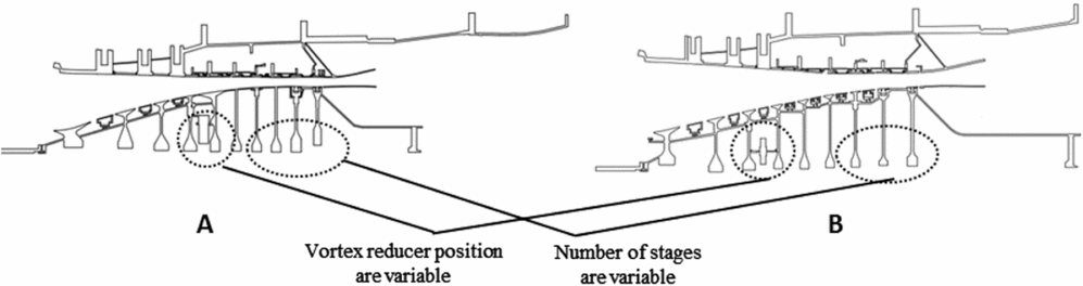
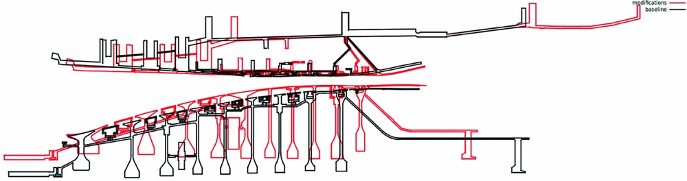
One additional observation is that, at least within the same model family, engine structure designs do not show large variations; rather, broad similarities can be identified. These similarities exhibit in both the geometric and physical models. For individual geometries, such as the blade discs, although differences lie at their lengths and widths, their structural layout (e.g., the shape skeleton) are the same. All discs can be modelled by using its centre-line configuration and its thickness distribution. Furthermore, as shown in Fig. 1, the high-pressure spool for engines A and B demonstrated large similarities although a number of differences in the details can be noticed, e.g., engine A has an extra HPC stage and the locations of the two vortex reducers are different. These observations suggest that at least some degrees of data re-use are possible when modifying the geometric and thermal model from a baseline engine to generate its variations. The second major contribution of this article therefore is to propose a method to enable fast geometry and thermal models regeneration by re-using previous designs. The enabling techniques include BCs parametrisation as well as their association to the geometric features; methods to automatically handle geometric changes and achieve fast data re-use, described in Sections 2 and 3.
The HPCs of engines A and B display large similarities but certain differences.

This article presents an approach that can significantly reduce the time-cost in preliminary thermal-mechanical design, which in nature is highly iterative and involves large number of boundary condition data. The methodology is built upon the feature-based system previously proposed by the authors(Reference Mare, Kulkarni, Wang, Romanov, Ramar and Zachariadis29) and allows sets of BCs to be represented parametrically. The parameterisation of BCs is associated to engine assembly features enabling the establishment of the one-to-one mapping between its geometric model and related thermal-mechanical model. Additionally, some heuristic rules are applied to allow the downstream analysis models to retain logical validity–if not physical accuracy–to accommodate geometric changes. A GUI is also developed to enable fast reuse of the features and their associated data, through the Drag-aNd-Drop (DND) operations conducted from one assembly to another. The capability of the approach is demonstrated by some challenging industrial applications. Although the approach is only represented in 2D, it can be readily extended to 3D gas turbine designs, considering that the geometries in gas turbine are largely axi-symmetric.
This article is organised as follows. Section 2 describes the methodology to build up the linkage between the geometric and thermal models using breakpoints. Section 3 describes how data are quickly re-used through the proposed breakpoints concept. Section 4 demonstrates the capability of the approach through some real industrial challenges. Finally, conclusion remarks are given in Section 5.
2.0 PARAMETRIC BOUNDARY CONDITION REPRESENTATION
2.1 BC configuration for component features
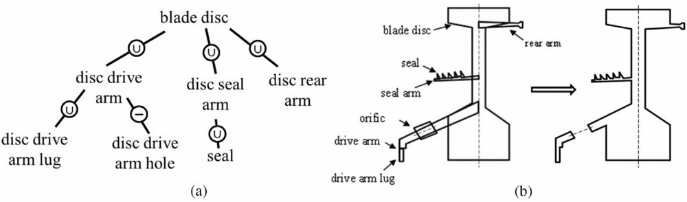
The authors previously presented a feature-based geometric modelling system for the representation of gas turbine assemblies(Reference Mare, Kulkarni, Wang, Romanov, Ramar and Zachariadis29). This system is based on abstraction. Starting from the most abstracted feature, that is the engine feature itself in its virtual form, the entire engine design is evolved by adding more detailed geometric information layers to the previous features as child features. A tree-like feature-based data structure, called a feature-tree is therefore formed. The layout of the feature-tree represents the engine design workflow. The features, although starting off at their abstract forms as building blocks which are devoid of functional information, are meant to be coupled with additional geometric elements at later stages for CAD visualisation and design purpose. Furthermore, they can be associated with physical properties for analysis at the downstream design and analysis phases on ad-hoc basis. The feature-tree is embodied through the General Assemble (GA), which is obtained by performing iterative Boolean operations to traverse the 2D geometric polygons represented by the features entities in the tree. Figure 2 explains how a drive cone, denoted as Ω dc , is assembled using its sub-features in the tree structure. The component is virtually assembled through Ω dc = fs ∪fd ∪fda ∩fo , where fs denotes a seal feature, fsd denotes a disc, fda denotes a drive arm and fo denotes an orifice. The section of the drive cone is formed by performing polygon union (∪) and intersection (∩) operations on the contours of its components. The same process is applied recursively throughout the assembly until the complete GA is formed. From a geometric point of view, the GA is a set of surfaces grouped by geometric primitives. However, this is not the case from the standpoint of physical modelling. For example, for the purpose of thermal analysis, the surfaces of the GA are grouped by BCs. The positions where the boundary groups begin and end are in general independent from the vertices of the GA. An intuitive way of handling this would be to assign BC data directly to each feature as the intrinsic feature parameters related to its geometric contours(Reference Thakur, Gopal and Gupta3,Reference Red, Jensen, Weerakoon, French, Benzley and Merkley30) .
Generation of a blade disc through feature-tree.

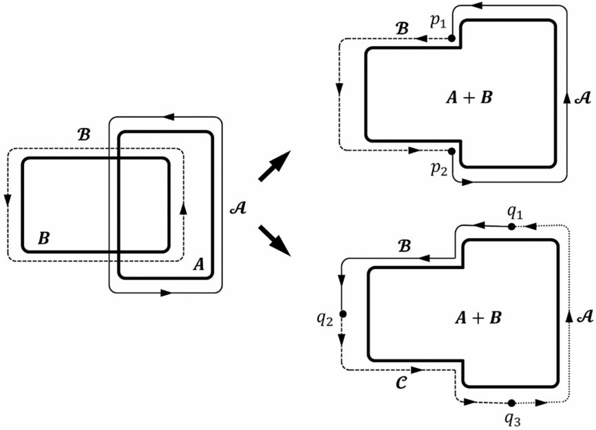
The idea of attaching BCs to the features seems trivial. However, to maintain the consistency and integrity for the BCs while permitting some automatic self-adjustments as per the design changes, particularly the topological changes, is not a straightforward task. Examples are shown in Fig. 3. Let two features (
A
and
B
) carry different sets of BCs which are then merged to form a new feature, where the BCs are labelled with script capitals (e.g.,
 $\mathcal{A}$
), and the features are labelled with Roman capitals (e.g.,
A
). Instinct will tell that if BCs are associated to features without human intervention, the boundary groups on the surface of the new feature should join these two BCs at the intersection points, p
1 and p
2. However, this assumption is not necessarily correct as a designer might wish to modify the positions of the boundary groups to the points q
1, q
2, q
3 instead – e.g., owing to the expected differences in flow patterns and heat transfer conditions. Some elegances need to be in place to guide the BCs’ action when it undergoes geometric modifications. In this article, a solution is proposed to introduce breakpoints along the feature contour in a parametric manner, which should split the feature geometric contours at arbitrary positions in order to achieve BCs’ regrouping. The data structure of the breakpoints and how they operate are elaborated in the next section.
BCs distribution after union of features A and B: with (above) and without (below) manual engineering expertise intervention.

2.2 Breakpoints
On the one hand, design practice in thermal-mechanical design suggests that a breakpoint may exist at an arbitrary position along the polygon contours. On the other hand, the split locations are most likely to be positioned at salient loci along the polygon contours, e.g., sharp corners. Also, the locations of the breakpoints tend to follow certain conventions, e.g., the breakpoints tend to stay at the corner of a feature component regardless of the size and dimension changes during the operating condition changing phase. Thus, the following characteristics should be demonstrated by the breakpoints:
-
• Associated with a specific type of feature;
-
• Mapped parametrically onto a feature, as per its geometric contours;
-
• Permits certain degrees of manual intervention; and,
-
• Associated with BC's information.
The inserting position of the breakpoint Bt (i) depends on the type of feature. This concept is best illustrated by the following two examples. One is a generic feature and the other is a labyrinth seal feature. It is worth mentioning briefly here that to create a full gas-turbine design and simulation suite, a feature taxonomy has been created in this research, where the generic and seal features are two examples in the taxonomy. One ideology we followed to create such feature taxonomy is based on abstraction: from the geometric perspective, the feature definition is substantiated from virtual to 1D, then to 2D and eventually progressing to 3D; and the feature types in the feature taxonomy are from generic to specific. Contrary to the MAT (middle axis transformation) method reported in the literatures( Reference Chong, Senthil Kumar and Lee 2 , Reference Thakur, Gopal and Gupta 3 , Reference Rezayat 16 , Reference Sheffer 31 ), the feature geometry is produced from a completely opposite route, i.e., from lower dimension to higher. By first defining its centre-line configuration, which gives the1D skeletal presentation of the feature, it then adds the thickness attribute to generate its 2D model. Eventually, 3D parameters, such as the distribution configuration of the holes along the engine circumference are specified to complete the geometric definition. The rationale behind this is to build a design-for-analysis CAD-CAE system where the dimensionally reduced or low-fidelity models are exploited to approximate the analysis result, thereby reducing the computational complexity expenses( Reference Robinson, Armstrong and Fairey 1 − Reference Thakur, Gopal and Gupta 3 , Reference Nolan 25 ). Nevertheless, the feature taxonomy falls out of the scope of this article, and it will be presented in our next publication, and hence will not be discussed in detail here.
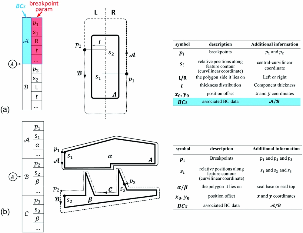
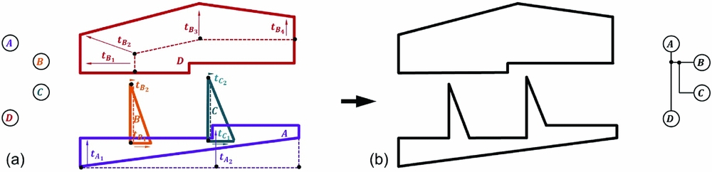
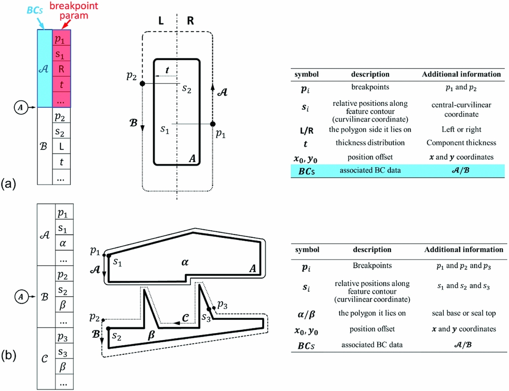
By examining the geometrical drawing of gas-turbine engine cross-sections, one may realise that most of the engine structural components are of the same category: they can be defined by the centre lines (structural skeleton) together with its thickness distributions (as the blade disc shown in Fig. 2). This type of feature is defined as a generic feature. The centre-line is not necessarily a straight segment and it could be a consecutive group of line segments (e.g., the seal abradable layer shown in Fig. 5(a)). The table on the right in Fig. 4(a) shows the properties of the breakpoints for the simplest generic feature. Let s denote the curvilinear coordinates along the centre-line, t denote the thickness of the feature geometry in 2D, L/R determine which side (left or right) the breakpoint is on with respect to the centre line. These parameters will generate a 1D Boundary condition layer creeping along the feature geometry contours. In addition, offset parameter (x 0, y 0) is introduced to offer the BCs an extra degree of freedom in the 2D plane. For example, one may wish to define a constraint at the position which is further away from the corner edge, where its location is not sitting exactly on the feature edge or surface as its 3D equivalent.
(a) Parametric breakpoint located with respect to the curvilinear coordinate of the feature centre line; (b) Parametric breakpoint located with respect to the feature contour.
(a) Sub-components, A : seal base, B and C : fins, and D : abradable layer; (b) Seal feature through union operation.
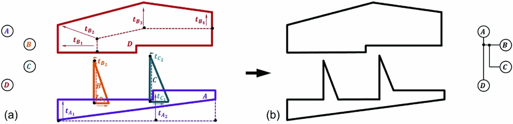
Although some types of features can achieve lower dimensionality through the use of intrinsic constrains and mutual relations among the their geometric primitives, and by decomposing the components into sub-modules, they are difficult to be defined by using the centre-line and thickness distributions. For example, the labyrinth seal shown in Fig. 5(b) is composed by several sub-components shown in Fig. 5(a) i.e., seal base (A), abradable layer (D), and two seal fins (B and C). A more effective solution we used here is to assign them with the BCs by walking through its geometric contours directly, provided that only low-fidelity analysis to the component is required. The insertion position of breakpoint Bt
(i) is defined by the curvilinear coordinate along its 1D contours (see Fig. 4(b)). The two examples,– generic and seal features, are illustrated in Fig. 4. The features are labelled with Roman capitals (e.g., A) and their boundary conditions are differentiated by their line styles and are individually labelled with script capitals (e.g.,
$\mathcal{A}$
). The tables on the left and right illustrate the intrinsic parameters of the breakpoints carried by each feature. The parameters include the breakpoints' identifier (pi
), relative positions (si
), polygon sides ((L/R) (i)) thickness (ti
), position offset ((x
0, y
0)(i)) and their associated BCs data (BC
(i)). For clarification, in the tables shown on the left, the breakpoint parameter section (displayed in red background) is not a subset of the BCs section (displayed in blue background), and both sections are the properties of a breakpoint.
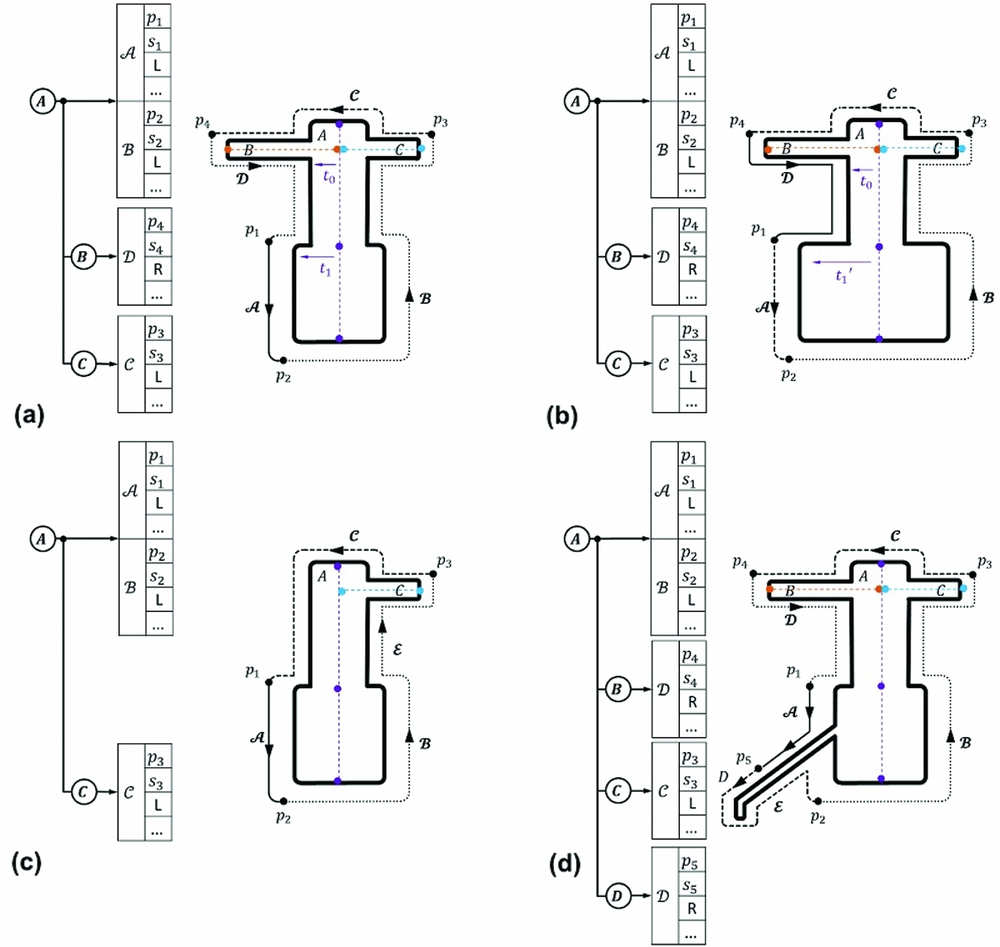
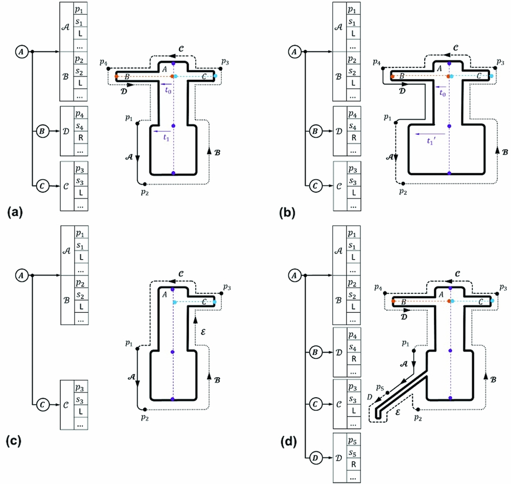
Automatic geometry adjustments according to feature dimensional changes are realized by assigning the parametric breakpoints along the geometry contours using curvilinear coordinates, either with respect to the centre-line for the generic feature, or along the 1D geometry contour boundaries for the complex features. As the two examples shown in Figs 6(a) and (b), while the breakpoint p
2 is located at the left-bottom corner, if the width of the feature is increased (from t
1 to t'1), the location of the breakpoint p
2 will be adjusted accordingly. To accommodate topological changes automatically, two heuristic rules have been implemented to handle feature and breakpoint removal and adding, defined as follows. Let the system collect the breakpoints for BCs intervals in a continuous manner, i.e., clockwise or counter-clockwise, along the closed 1D polygon contour boundaries. For feature removal: Fill the gap created by the deleted feature along the 1D contour boundaries by propagating through the BC configuration defined by its precedent breakpoint until it meets the next remaining breakpoint (compare Figs 6(a) and (c)). For feature insertion: Insert the new BCs carried by the new breakpoints into the existing 1D contour boundary. Starting from the newly inserted breakpoint, the boundary will be covered by the new BCs until it meets the next remaining breakpoint along the 1D contour (compare Figs 6(a) and (d)). Such logic also stands true when breakpoints are being removed/added from/to the features. These processes are referred to as BC healing for feature topological changes to prevent any undesired BC gaps. Besides, boundary sections can also be assigned as void by defining the BCs as void type to state that the covered sections have no specific BC being assigned. In Fig. 6, features are labelled with roman capitals (e.g., A) and boundary conditions are differentiated by their lines’ styles and are labelled with script capitals (e.g.,
$\mathcal{A}$
). The status tables are displayed in a hierarchical manner in line with the topological relations, and hence displaying in a feature-tree structure. Each node in the tree denotes a feature. For more information about the feature-tree, readers can refer to.Ref. Reference Mare, Kulkarni, Wang, Romanov, Ramar and Zachariadis29.
(a) Baseline geometry; (b) Dimensional change; (c) Removal of feature B ; (d) Addition of feature D .
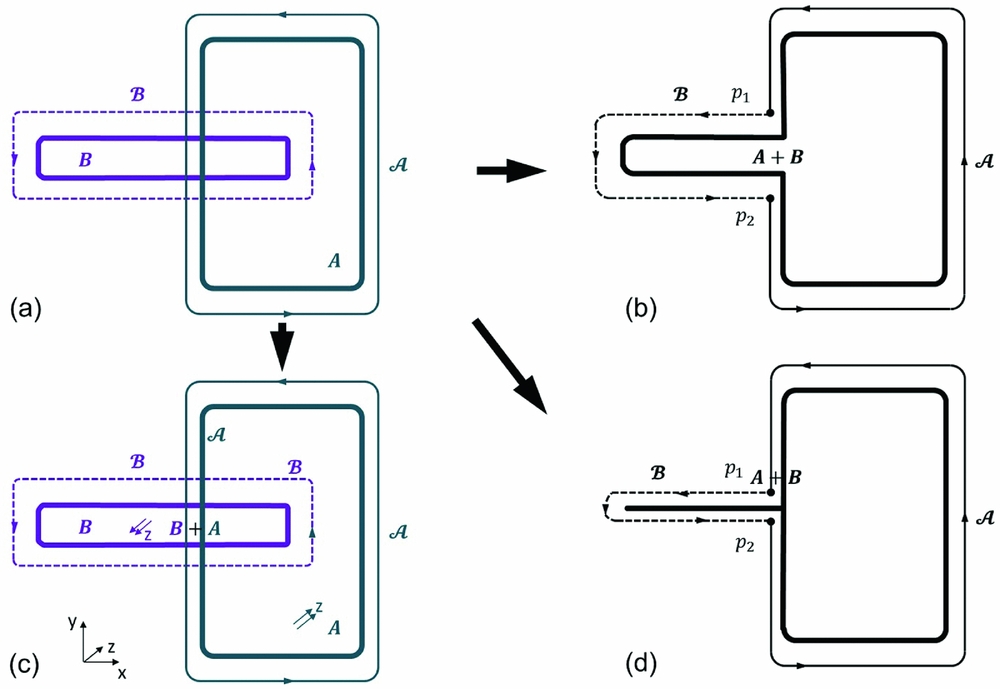
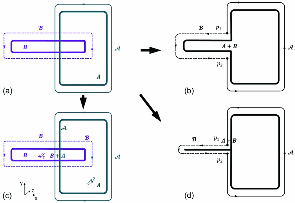
It is worth emphasising that the method is generic and also applicable to the non-manifold design need. Non-manifold design has gained increasingly interests in recent CAD-CAE development community. Some of its benefits are described by Refs. Reference Thakur, Gopal and Gupta3, Reference Hun4 and Reference Nolan25. The method proposed in this article should be able to be wrapped into the non-manifold design environment seamlessly. Figure 7 lists some examples. While Fig. 7(b) shows how the method automatically sews the BCs carried by the two feature entities showing in Fig. 7(a) together when they undertake feature union operation in a normal manifold design setting, Fig. 7(c) and (d) demonstrate that how the method reacts in the non-manifold design cases. Figure 7(c) represents a component which consists of two adjacent volume (two faces in the 2D equivalence) cells, where in the 2D x-y design plane, these two cells are partially overlapped and glued together. In 3D space, one possible configuration of which can be that the two volume cells are facing and extruded at opposite directions, respectively, along the through-plane direction z, where a different thermal-mechanical BC condition is applied to each cell. Although the non-manifold design capability has not yet maturely developed in the commercial available CAD design tools to build a geometric feature entity like this, a quick work-around of reproducing such a case on these CAD platforms is to decompose the feature into two as geometrically coupled child features, A and B , and by turning off the polygon union operation during its assembling process. As such, by assigning the two individual BCs to each child feature, the method described in this article can successfully propagate the BCs throughout the 1D geometric contours separately, representing two different design domains on this joint feature. Furthermore, Fig. 7(d) illustrates a typical multi-dimensional non-manifold design scenario, where the 1D beam feature B represents a sweep-able thin sheet component in 3D. It can be seen that the 1D BC boundary works just as good as on the 2D geometric surface when it is applied on the simplified 1D geometry entity. In 3D, however, the 1D BC boundary should be swept into a surface as appropriate.
(a) Two sample features A and B; (b) Wielding A and B together as one coherent geometric manifold piece; (c) Overlapping two features as two non-manifold geometric piece joint together; (d) Non-manifold multi-dimensionality design environment.
2.3 BC healing to accommodate design fidelity and resolution changes
The method proposed above provides a significant advantage when the geometry undertakes design fidelity and resolution changes, e.g., level of detail (LOD) and level of abstraction (LOA) modifications. Changes of LOD and LOA are the two common practices taking place within the CAD-CAE design pipeline. In a conventional iterative design cycle, on the one hand, the LOD process produces a simplified CAD model for the CAE process, where some geometric details (such as small-sized holes or fillets) are removed to reduce the mesh size. On the other hand, the LOA process is required when a more detailed analysis is to be produced (e.g., study the impact of the additional fillet features to the stress analysis)(Reference Robinson, Armstrong and Fairey1-Reference Thakur, Gopal and Gupta3,Reference Foucaulta, Cuillirea, Franoisa and Maranzanac20,Reference Tierney26,Reference Tierney27,Reference Lee, Armstrong, Price and Lamont33) . To achieve design fidelity and resolution changes, the conventional approaches are usually cumbersome and labour-intensive, and often require considerable engineering expertise. To overcome these challenges, some researchers introduced a common data model as a data bank which hosts all the data required for both the CAD and CAE process( Reference Hun 4 , Reference Gujarathi and Ma 34 , Reference Tierney, Nolan, Robinson and Armstrong 35 ). Such models can generate detailed CAD and simplified CAE models immediately as ad-hoc manner. Other researchers attempted to compile a central data file to establish the link among different models with fidelity variations(Reference Lidong36), where the file acting as an independent data structure for information exchange between geometric design and FE analysis phases. Although these approaches simplified the transition during model fidelity and resolution change phases, they inevitably generated computational overheads by creating and maintaining these common data models and data structures. However, the proposed method in this article bypasses the need of generating an additional model via coupling the BCs through integrating the BC representation with the feature geometry presentation, where the BCs are embedded into the geometric contours as internal parameters. The implemented BC healing rules allow the BCs to be automatically adjusted in response to design fidelity and resolution changes, through the use of geometric properties, e.g., curvilinear coordinates.
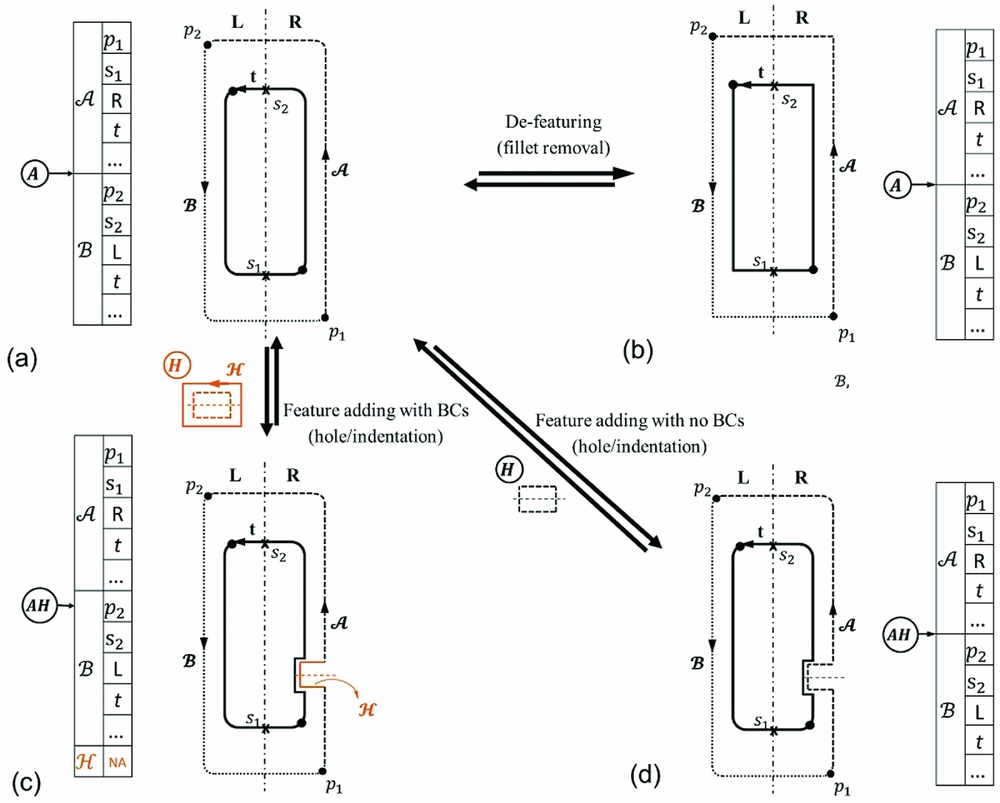
Two examples are selected to demonstrate the proposed approach handling fidelity and resolution changes. In the first example, the feature undergoes design resolution changes, where the fillets of the feature in Fig. 8(a) are removed or added. When the fillets are removed, the BC boundary will be automatically reshaped and updated to accommodate the change to derive the analysis (e.g., thermal-mechanical) model. The 1D BC boundaries will automatically cover the newly generated feature contours by propagating from one breakpoint to another (Fig. 8(b)). In Fig. 8(b), the centre-line is oriented from bottom to top. As a result, breakpoint p
1 lies at the bottom of the feature, where s
1 = 0. R indicates it lies at the right side of the centre line, and t is the thickness.
$\mathcal{A}$
is the BC information carried by the breakpoint p
1. Similarly, p
2 is at the top of the feature, with s
1 = 1, L indicating it lies at the left side of the feature, and
 ${\cal B}$
is the BC it carries.
Illustration of BCs adjusted automatically after modification of geometry fidelity and resolution. (a) Fillet removal/restoration; (b) Adding/removing a void hole feature; (c) Adding/removing a hole feature carrying BC representing flow condition.
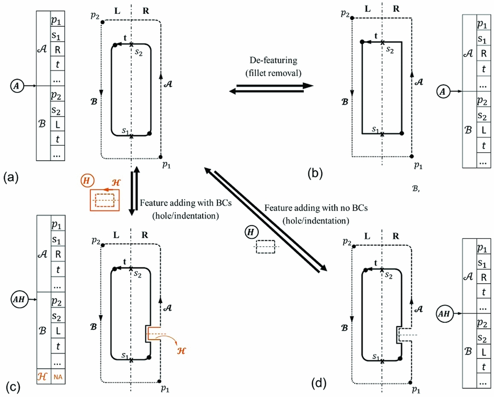
In the second example, the feature undertakes design fidelity changes, where the small-sized feature, an orifice H in this example, is added or removed. The example shows that the method can automatically cover the cut-through area by the BC carried by the precedent breakpoint along the 1D geometric contour (Fig. 8(d)). Please note, these two operation examples shown here are both bi-directional, i.e., from lower fidelity or resolution to higher, and the opposite way. Having demonstrated the effectiveness of the method by these two simple examples, enhanced design automation can be achieved. For example, in the example given in Fig. 8(c), the cut-through area has not specified with any additional BC to separate the flow field from the solid geometry surface (3D equivalence). One alternative way is to assign the orifice H with a specific BC representing its flow condition. As such, the cut-through area will be covered by the new BC
 ${\cal H}$
. These additional design rules can be introduced into the system when necessary. On the one hand, additional design automation may enhance the design efficiency; on the other hand, it may defeat its generality where the design requirements may change from one to another during the design course. Thus, here we keep the rules simple and generic but open to future alterations or improvements for individual design purpose.
3.0 DATA RE-USE
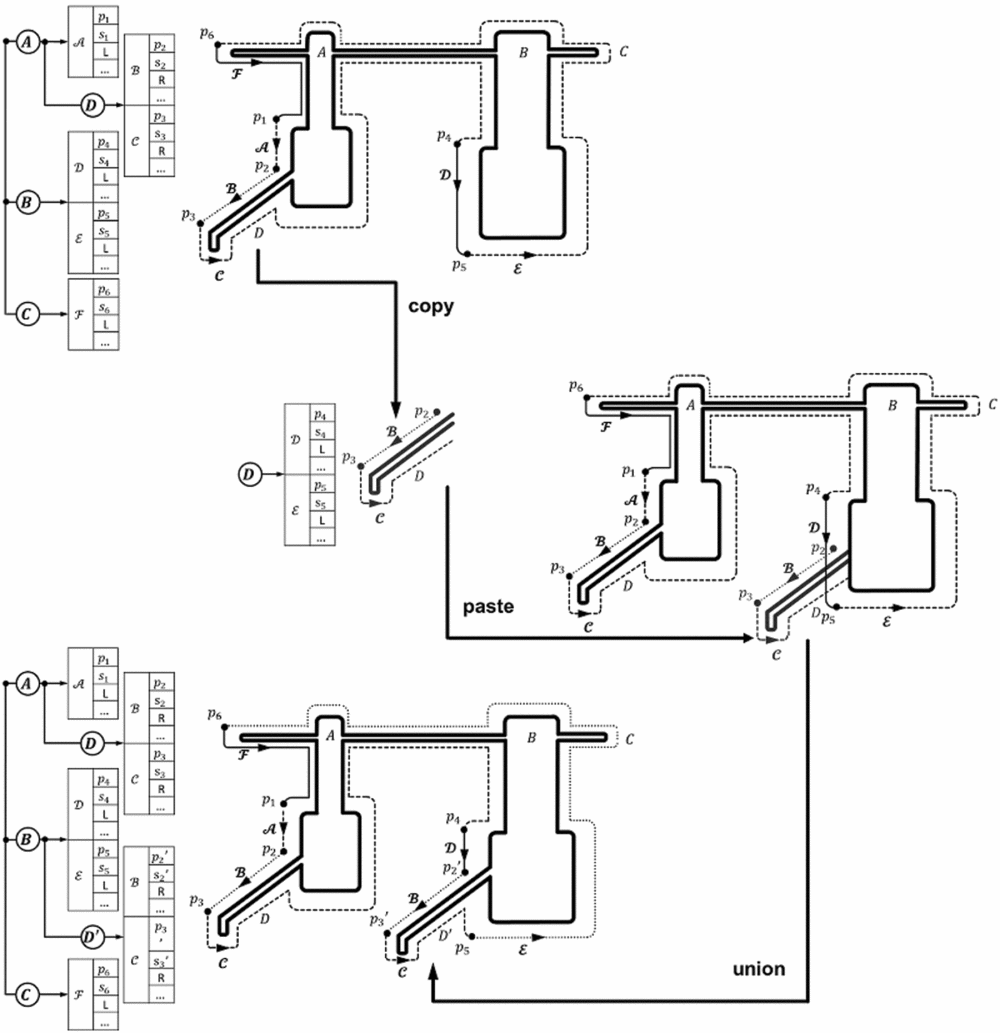
As mentioned in the introduction, much design knowledge should be shared and re-used for similar engineering products. Particularly for thermal-mechanical design and modelling, re-use both the existing geometric data and boundary condition data are favourable. To “insert” existing designs into the current new design and simulation models so as to promptly initiate new analysis loop to evaluate the new design is an attractive design route. The re-use of design and data can be easily achieved herein based on the described feature-tree and breakpoints methodology. Figure 9 illustrates the process of copying a drive-arm feature D from feature A and then pasting it onto feature B . As internal parameters, the breakpoints located on the contour of feature D are kept during the copy and paste process, and merged into the feature tree of feature B as child feature's attributes through feature union. Here we refer to union as Boolean union operation, and whenever the geometric changes are taking place, as soon as the geometry of the features need to be generated, e.g., visualisation purpose, the geometry of the features will be recomputed to produce a new geometry result. From the figure, it can be seen that feature D is copied where its duplication is inserted into the new host feature, feature B . Such operation will produce a new geometric entity where the BCs will be reconfigured automatically. As shown in the feature-tree chart on the left of Fig. 9, for the newly generated geometry, feature B carries the duplicated feature D as a child feature. (a new name D′ is given to avoid confusion).
Illustration of data re-use.

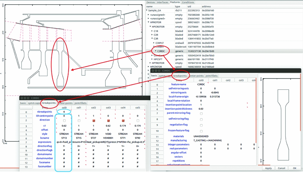
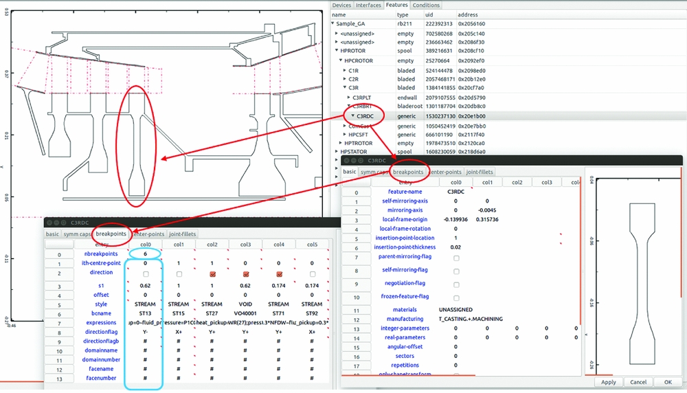
Although the data re-use method proposed in this article is generic and should be able to be realised through interfacing with other standardised CAD APIs, the benefit of this approach herein has been enhanced by a dedicated GUI developed for this research. The structure and topology of the feature-tree can be visualised and manipulated through the GUI. The GUI is developed in C++, utilising GTK design toolkit. As shown in Fig. 10, the GUI contains two panels, where the GA draws on the left, and the feature-tree denoting the topological structure of the feature is shown on the right. Any geometrical modifications to certain features will propagate throughout the feature-tree and will result in automatic updates of the GA drawing on the drawing panel. Each node in the feature tree represents a feature in an engine. The nodes can be accessed by their keyword, i.e., feature name. By clicking a feature node, the relative data associated with such feature, e.g., embedded breakpoints, will be displayed in a pop-up menu. Within the menus, the breakpoints are displayed in a separated tab page. Figure 10 highlights a blade disk which contains six breakpoints along its geometric contour. As shown in tab page 2, the six breakpoints are displayed in columns, with its BCs information listed vertically along each column. From the top to bottom, the thirteen parameters are: number of breakpoints in total associated to this feature, ith index of the centre-line skeleton point the breakpoint is associated to (for example, the p 1 in Fig. 8 will have index 0 and p 2 will have index 1), direction of the breakpoint (L/R), curvilinear coordinate, offset (x 0, y 0), and the rest of the rows are the attached BC information, which include the style, name, expressions – i.e., temperature and rotating speed – two directional flags, domain name and number, face name and number, of the BC. The GUI enables the user to add, remove or perturb the sequence of the feature nodes, whereby the breakpoints will be re-allocated accordingly. To insert a breakpoint, it can be done by increase the number of breakpoint parameter through the GUI, and it will automatically generate an additional column as an extra breakpoint placeholder. The inserted point can be specified based on the position along the feature contour parametrically. Conversely, removing breakpoints will need to decrease the number. Copying or re-locating a feature node from the tree will automatically copy and transfer this same feature together with its child features, including the associated parametric breakpoints, whilst the drop operation is equivalent to paste. By so doing, the previous design, existing in the form of assembled features, are able to be re-used and re-configured quickly, including the attached breakpoints and their BCs.
Demonstration of the GU.
4.0 RESULTS
The capability of the method is demonstrated by a set of industrial applications as follows. Test case 1 shows the reproduction of a simple baseline geometry and its automatically derived thermal model by using the feature-tree and breakpoints described in this article. Test cases 2–4 demonstrate how the BCs in the thermal models are updated automatically as per dimensional changes, feature removal and insertion. Test case 5 presents a challenging case representing a realistic HPC thermal-mechanical model redesign scenario, where a whole HPC is re-designed and the BCs are updated automatically to generate a model ready for meshing and the downstream analysis (e.g., FEA). Test case 6 shows the applicability of the method in the scenario of redesigning a secondary air system (CFD). The original geometric and thermal models are all given by the industrial funding body of this research.
4.1 Reproduce the baseline geometry geometric and thermal model generation
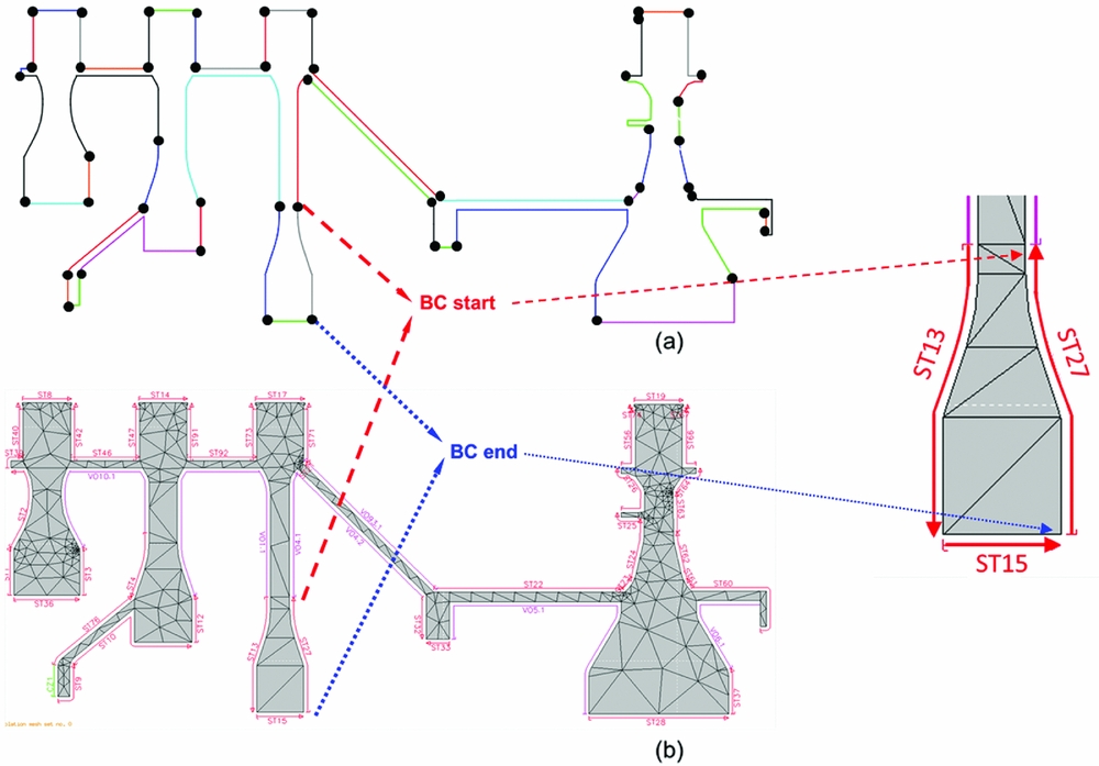
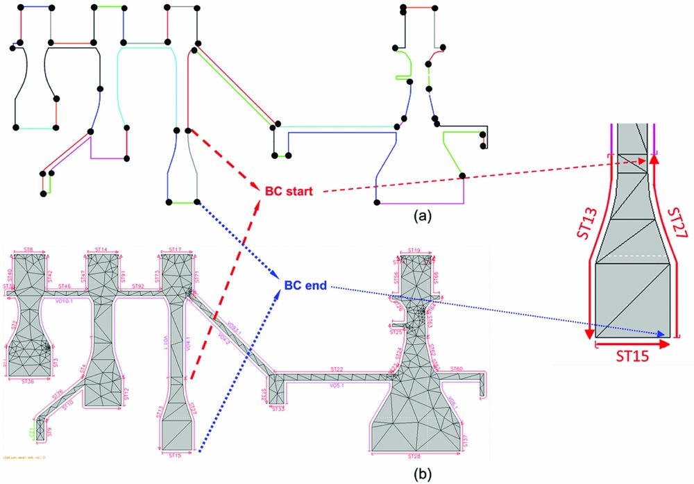
The baseline geometry and its thermal model presented here represent an idealised high-pressure spool in a gas turbine engine (see Fig. 11(a)). The geometry and thermal model have been re-created in our system based on the described feature-tree and breakpoint method. The original baseline GA was created in a commercial CAD software by connecting the vertices through low-level primitives, such as lines and arcs, to form the GA contours, thus neither mechanical nor topological rationale was available. To reproduce the GA and the thermal model, all the geometric assemblies have been dismantled into connected features (assemblies) and are reassembled into as connected features based on their topological and mechanical connectivity according to the described feature-tree method. For example, a blade disc is dismantled into as the features of blade disc, drive arm, drive arm lug, and so on (see Fig. 2). The locations of the breakpoints are re-parameterised as per the feature geometric configuration based on the parametric breakpoint method described in Section 2.2, and are assigned with specific BCs according the original given thermal model. These breakpoints are then mapped onto the features accordingly to reproduce the thermal-mechanical model. In Fig. 11, the breakpoints are highlighted as black dots where every two consecutive breakpoints specify a boundary group interval. The BC groups are displayed in different colours only to distinguish them from their immediate neighbouring groups, and the BC groups displayed with the same colour may not necessarily carry the same BC configuration. Each breakpoint carries the specific BC information needed for the thermal analysis for the segment it leads. Each boundary group is assigned with a unique tag. The tag is in the form of a character string. Representing the type of the BCs, the strings can be Streams (ST) or Conduct Zone (CZ). The string is followed by an integer, which is the index of the boundary section (e.g., ST18). Directional flags are also assigned to each boundary group. The final reconstructed thermal model from the baseline geometry is loaded into a proprietary FEA software which is routinely used in a major aero-engine company. The resulting thermal model is demonstrated in Fig. 11(b). To reproduce the first baseline geometry and thermal model based on the proposed feature-tree and breakpoint methodology is the most time-consuming step in this design flow, and it took a dedicated software engineer 2 man-hours to complete. The system runs on a 64-bit version of Linux GNU Ubuntu 14.10, with Intel Core i7 2.0 GH CPU and 8G RAM. The baseline geometric model is recreated by 82 feature entities, and the thermal model contains 53 BC sections and this turns into 53 breakpoints in total.
Test Case 1. (a) Baseline geometry; (b) Baseline thermal model.
4.2 Geometric and thermal model re-generation through data re-use
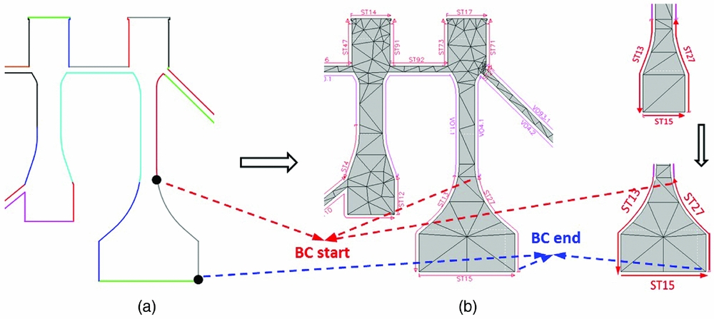
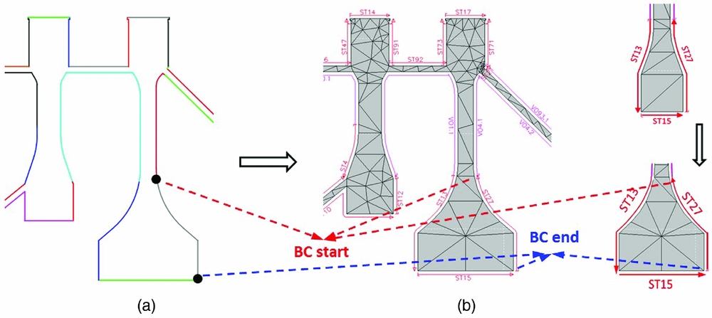
Fig. 12(a) demonstrates how the thermal-mechanical model reacts to the dimensional changes of the geometric model – in this case, increasing the turbine disc width. For traditional design routines, boundary conditions have to be re-configured and re-assigned manually when the geometry undergoes any changes, even for a small correction such as increasing the size of a disc. The elegance of the method demonstrated here in Fig. 12 shows that it can automatically re-shape and re-configure the BCs after the dimensional changes made to the geometry. The computation cost in the BCs update depends on the computational efficiency of the geometry kernel. For the current implementation, it takes 8 seconds to generate the new geometry and thermal models. Besides, current method successfully preserves unaffected BCs and automatically adjusts the rest boundary conditions after this dimensional change. The resulting thermal model with its boundary tags is shown in Fig. 12(b).
Test Case 2. (a) Baseline geometry with expanded 3rd disc; (b) Thermal model.
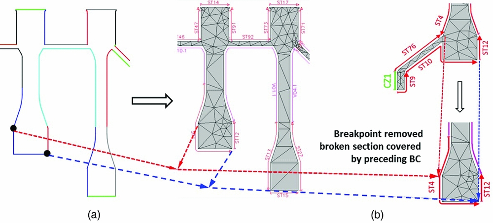
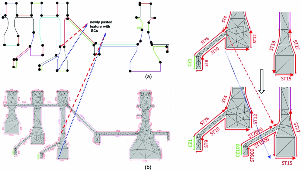
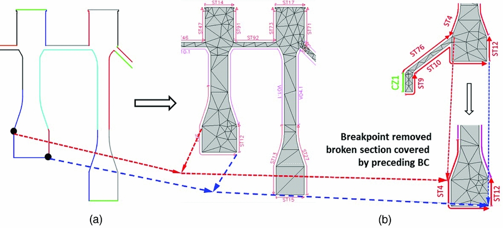
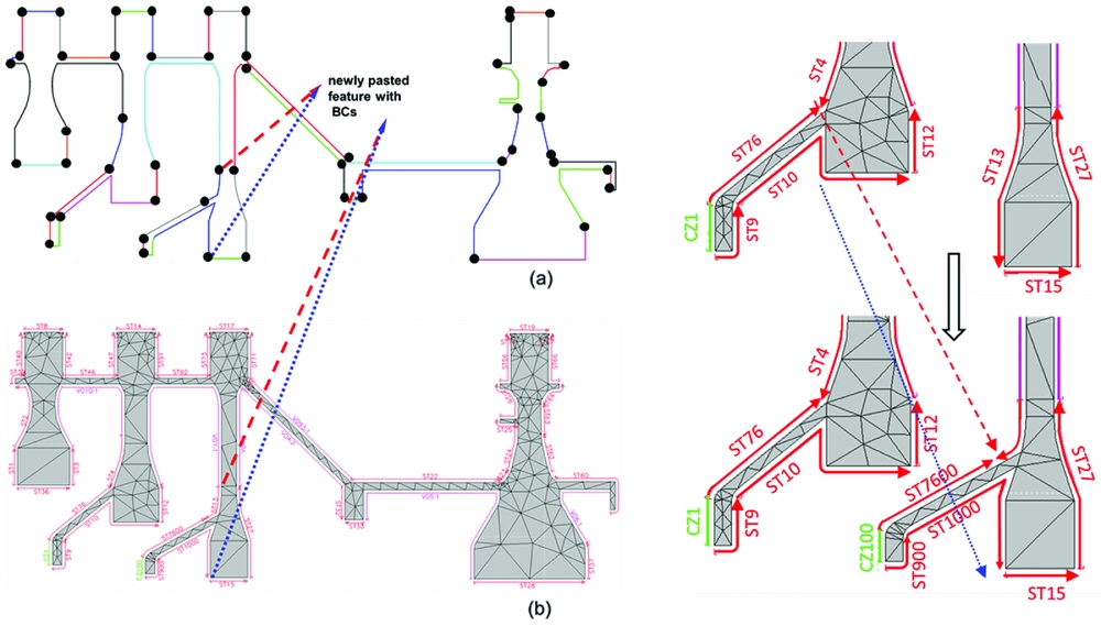
Test cases 3 and 4 demonstrate the BC healing and reconfiguration capability when the geometry undergoes topological alterations (e.g., feature removal and insertion). For the removal operation, as shown in Fig. 13, the drive arm feature has been removed from the second disc (see Fig. 13(a)). This will generate a void gap between the removed section and the next adjacent breakpoint. No boundary condition would be available across this gap. For the traditional design process, engineers have to manually fill in this gap with specified BCs. However, the proposed system heals the void section by covering it with its preceding BC data automatically (see Fig. 13(b)). For feature insertion operation, the drive arm feature is copied from the second bladed disc and pasted onto the third one. As shown in Fig. 14, copying the feature will simultaneously transfer its boundary conditions to the new host feature. The new BCs joined with the existing BCs of the host feature correctly, where the tags of the new BCs are appended with zeros to avoid duplicity. The copy-and-paste operation is accomplished by the dedicated GUI developed for this research. This design cycle takes a dedicated software engineer 10 seconds to complete.
Test Case 3. (a) Baseline geometry with removed drive arm on 2nd disc; (b) Thermal model.
Test Case 4. (a) Baseline geometry with the drive arm feature copied from the 2nd disc onto the 3rd disc; (b) Thermal model.
4.3 Numerical analysis model regeneration based on data re-use
Test case 5 shows the FEA model regeneration based on a more realistic configuration. The baseline and modified configurations are the realistic representations of potential turbofan High-Pressure Compressor (HPC) designs. The annulus dimensions are however distorted to protect proprietary design knowledge.
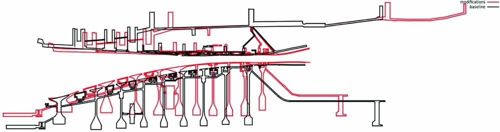
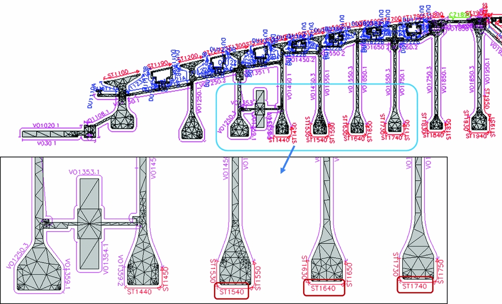
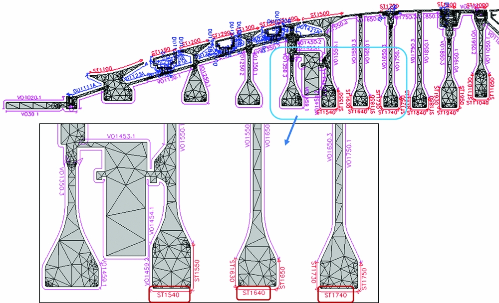
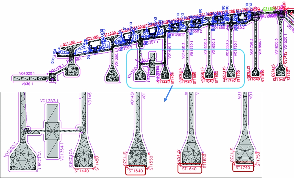
The workflow starts with the re-creation of the baseline geometry and thermal models in our developed system, based on the models supplied by an aero-engine company. As shown in Fig. 16, the reproduced thermal model is in the form of 1D boundary condition sets creeping along the 2D geometry model contours. These thermal boundary condition sets are delimited by breakpoints with their directions are being displayed as the arrows in the plot, and are tagged with specific BC names. The baseline engine is modified and its design configurations are re-used as much as possible to quickly generate a new design of such engine family. The redesign operation involves modification of the annulus lines, insertion of a new stage (stage 10 in Fig. 17), a number of dimensional changes (e.g., increase or reduce blade width, adjust the blade disc height), as well as topological changes on some of the assemblies (e.g., transfer the vortex reducer from stage three to stage four) (compare Figs 16 and 17, as per Fig. 15). The transformation is achieved using the dedicated GUI described in Section 3. Most of the new geometry is generated by copying the components from the original assembly and morphing into the new assembly, where the new engine only contains a set of annulus line detention and no other geometric part in the first place. The re-used components are pieced together following their topological order and are automatically conformed to the shape of the new annulus lines. Although in the process of re-use existing engine configuration, e.g., copy-and-paste from one engine to another, most of the engine model regeneration work is automated, the system permits the user to make adjustments at any time during the process, if necessary. These include the modifications made to the feature geometric parameters, e.g., the thickness, or to the parametric location of the breakpoints and their associated BC data. After both the baseline and modified geometric and thermal-mechanical models are regenerated, they are finally imported into a FEA solver to undertake thermal analysis. The resulting analysis models are shown in Figs 16 and 17.
Test Case 5. Comparison between the baseline and modified engine HPC geometries.
Thermal model of the baseline engine HPC.
Thermal model of the modified engine HPC.
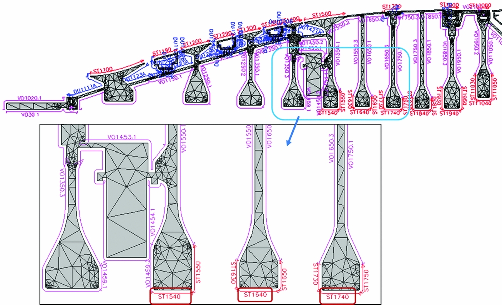
The entire redesign process took 9 man-hours to complete, including 5.5 man-hours to recreate the original GA model as features, 1.5 man-hours to regenerate the breakpoints and BCs using our proposed method, and 10 seconds to generate the GA geometry and its thermal model in the developed system (wherein a formatted data file contains thermal BC configuration for thermal analysis is created), and 2 man-hours to morph the existing models into the new geometry and thermal modes). Please note, such practice conducted by the traditional design paradigm could take several months in a major aero-engine company, taking into account that coordination needs to be in place between the geometric design team and thermal analysis team, as well as the iterative nature of the design cycle. This is due to the large number of geometric entities (geometric component features in this model) and BCs (BCs in the thermal model) in this model. By using the concept of breakpoints, majority parts of the GA and BCs in the baseline model (such as the highlighted ST 1540, ST 1640 and ST 1740 on the blade discs) are recycled, and most of BC intervals are automatically adjusted to adapt to the geometric changes and are mapped onto the new model. The BC groups are differentiated by their BC names: initialed with the BC type, such as stream (ST), and are followed by its numerical identifier, such as 1540 in the figure. In this testing case, the vertex reducer is shifted from stage three onto stage four. The result shows that with its associated BC data recycled, the BC tag is renamed manually from VO1353.1 to VO1453.1 to maintain the naming consistency in accordance to its parent features and its stage number. (VO means the BC type is of void zone).
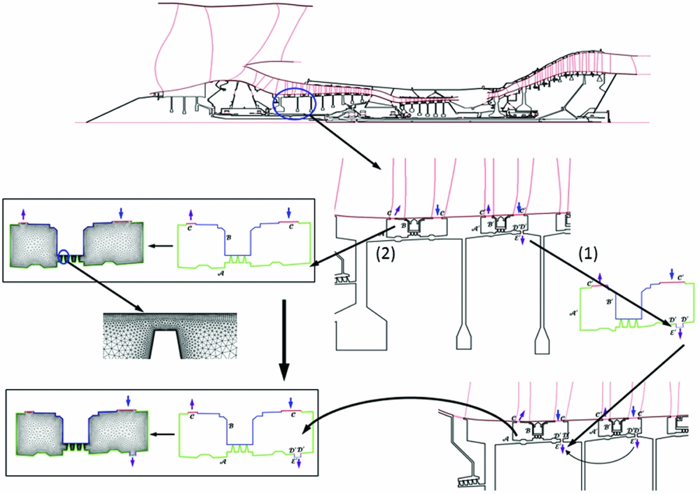
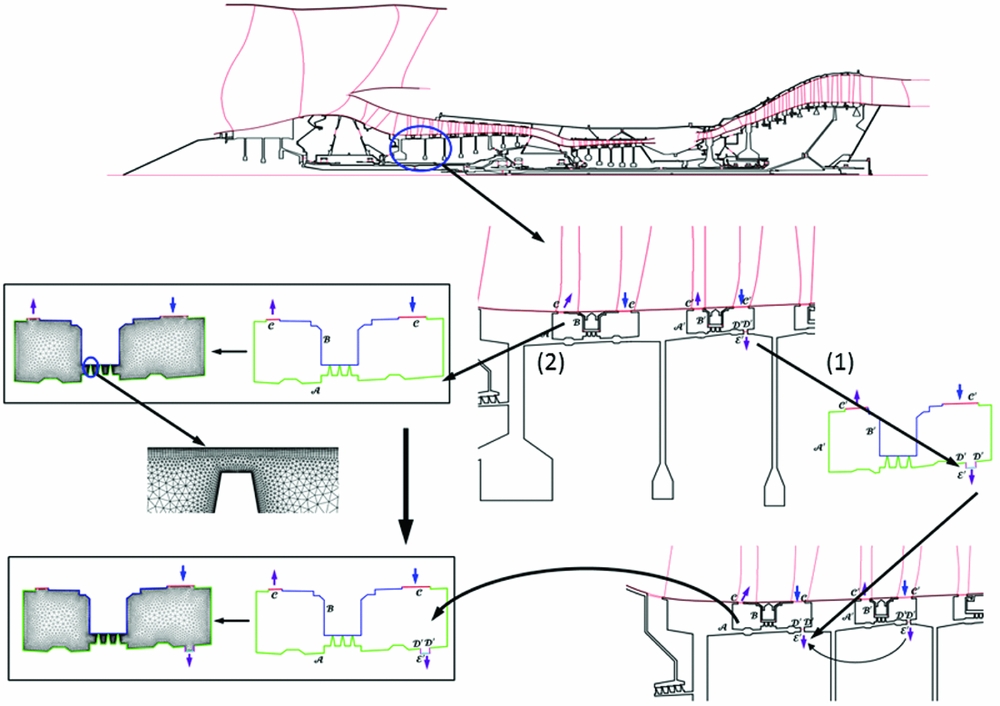
Test case 6 demonstrates the capability of the method being applied in CFD analysis domain, i.e. rapid CFD model generation for the secondary air system. As shown in Fig. 18, compared with the original IP stator cavity, the intended stator cavity added an extra orifice together with its BCs named as D′,
 and D′, where D′ specifies the condition for the walls and
for the air outlet orifice. Within this practice, the designer copied the orifice from the cavity (1) and pasted it onto the cavity (2). The result showed that both the orifice feature geometry, and its BCs are copied onto the cavity (2) correctly and forms a closed-loop BC configuration. The new CFD mesh(Reference Wang and di Mare37) is thus generated automatically and ready to be used for the new CFD simulation cycle.
Test Case 6. Illustration of data reuse in the secondary air system.
4.4 Discussion
From the test cases, it can be seen that, in the proposed design framework, to create (or reproduce) a first baseline model from scratch by using our feature-tree method and to associate the breakpoints with the BCs to generate the thermal model are the most time-expensive design phases in the workflow. The workloads are similar to, or can be even heavier than that of, using conventional CAD design systems. For example, in SolidWorks, a user can first insert all the vertices at the suitable places, and then connect them using lines, splines arcs or the like to form the closed polygons. Such design processes can be quicker than the feature-tree method presented herein. For instance, the GA shown in Fig. 10 can be created in SolidWorks in less than 60 minutes, whereas it took 2 man-hours to reproduce the model using the proposed methodology described here. However, the advantage of the proposed method becomes significantly pronounced in the following iterative design phases. This can be explained by a simplified mathematic model. Let the workload required to create the first initial baseline geometry and thermal model using conventional design tool define as w 0. As a crude approximation, we can also assume the workload of using the proposed approach to be w 0 as well (at least of the same magnitude). Let the number of design iterations be defined as n iter. As for the conventional design flow, each iteration will require a similar workload in the worst case; hence, the total workload W = w 0 + w 0 × n iter grows linearly as per the number of iterations. On the contrary, for the proposed method in this article, the workload can be as low as a constant of W' = w 0 + 0 × n iter = w 0 for the ideal cases, where no extra modification is required (in other words, all features are directly re-used). In the realistic cases, however, the complexity would be W' = w 0 + w 0 × (1 − R) × n iter, where R is the data re-use rate. Thus, a high data re-use rate in an iterative design environment will demonstrate a significant advantage against the traditional design approach
5.0 CONCLUSIONS
This article presents a novel approach which is able to considerably reduce the time-cost in thermal-mechanical design of gas turbine engines. Typical thermal-mechanical models involve large numbers of components with complicated geometries. Due to the missing link between the geometry and its boundary conditions, the re-generation process of suitable downstream analysis models is a cumbersome and formidable task, where the assignment and update of boundary conditions after geometrical change is difficult and time-consuming. This article describes a method to bridge the gap between the feature component geometry and its associated boundary conditions. The method is demonstrated to be able to update the BCs automatically to adopt the geometric modifications. These modifications include both the dimensional and topological changes. Enabling techniques in the proposed approach include feature-tree representation of the engine assembly parts and their topological relationships, BCs assignments to the features through parametric breakpoints, automatic BC healing and re-configuration to adopt geometric changes, and data re-use for new geometric and analysis models generations. The proposed methodology is generic and can be easily realised through standard CAD-CAE package APIs, and it is applicable even to non-manifold and multi-dimensional design environment. Its advantages are demonstrated through our in-house implemented design system with its dedicated GUI interface. The three test cases are: (a) to derive new design configurations from an idealised HPC model, (b) to morph an existing HPC spool into a different configuration, and (c) to re-use part of an IP stator cavity model. The test cases demonstrate that the system is able to adjust the BCs coverage automatically in response to the dimensional changes, and is able to heal the BCs to meet the topological and design fidelity and resolution changes. Further, freedom is given to permit human interventions at any time during the design pathway, which can be gained through the dedicated GUI. The results, particularly for the applications of realistic industrial design cases with iterative design nature, are very encouraging. A rapid thermal-mechanical and CFD model regeneration is achieved, which cuts the design time expense by at least one order of magnitude.
Future direction of this research work will focus on implementing data re-use on the whole engine design and simulation scale and to build a virtual wind tunnel for gas turbine engines. From the proof-of-concept results demonstrated in this article, we argue that to bridge the CAD model and its downstream analysis models through associating parametric breakpoints with the assembly features is a useful strategy to achieve design automation and should be included in the future CAD-CAE design and simulation toolsets. Thus, to test the proposed approach in other commercialised CAD packages and apply it in other design spaces, such as the 3D applications, would be interesting, where the 1D BC boundary and 2D geometry contour should be extended to 2D BC surface and 3D solid or shell or as such, respectively.
ACKNOWLEDGEMENTS
The authors gratefully acknowledge Rolls-Royce plc and the EU Clean Sky programme for funding this work and authorising its publication. The authors also sincerely thank the anonymous reviewers, whose comments have significantly improved this manuscript.