1. INTRODUCTION
The modernisation of Global Navigation Satellite System (GNSS) signal structure plays an important role in the development of GNSS. In the process of Global Positioning System (GPS) signal modernisation, not only new civil signals L1C (Betz et al., Reference Betz, Blanco, Cahn, Dafesh, Hegarty, Hudnut, Kasemsri, Keegan, Kovach, Lenahan, Ma, Rushanan, Sklar, Stansell, Wang and Yi2006), L2C (Fontana et al., Reference Fontana, Cheung, Novak and Stansell2001), and the authorised M code signal (Betz, Reference Betz2000) have been added to the L1 (1575·42MHz) and L2 frequencies (1227·6MHz), but also a new frequency L5 (1176·45MHz) and new L5C signal (Spilker and Van Dierendonck, Reference Spilker and Van Dierendonck1999) have been added. A significant feature of these modernised GNSS signals is that each service signal includes a data component and a pilot component. For example, 75% of power in the L1C signal is allocated to the pilot component (Betz et al., Reference Betz, Blanco, Chan, Dafesh and Hegarty2007). Multiple signal components need to be transmitted at the same frequency, but the power of the satellite payload is limited. In order to maximise the efficiency of the High-Power Amplifier (HPA) and reduce the distortions, it is preferred that the signal envelope is constant (Dafesh and Cahn, Reference Dafesh and Cahn2009). Therefore, single-frequency constant envelope multiplexing methods are proposed, including the Interplex (Butman and Timor, Reference Butman and Timor1972), Majority Vote (Spilker and Richard, Reference Spilker and Richard1998), Coherent Adaptive Subcarrier Modulation (CASM) (Dafesh et al., Reference Dafesh, Nguyen and Lazar1999), Phase-Optimised Constant-Envelope Transmission (POCET) (Dafesh and Cahn, Reference Dafesh and Cahn2009) and quasi-constant envelope multiplexing (Yan et al., Reference Yan, Tang, Wei, Qu and Zhou2015). These methods can meet the demand for single-frequency constant envelope multiplexing of GNSS signals. In order to keep the envelope constant, useless Inter-Modulation (IM) terms are introduced, which causes power loss. Multiplexing efficiency is usually used to evaluate the performance of constant envelope multiplexing methods. The multiplexing efficiency is defined as the ratio of the power sum of useful signal components to total power (Fan et al., Reference Fan, Lin, Wang and Dafesh2008).
With the evolution of GNSS signal structure, GNSS signal design has a need for Dual-frequency Constant Envelope Multiplexing (DCEM). The signal components at two adjacent frequencies are combined into a constant envelope signal. The significant advantage of DCEM is that it can reduce the signal distortions and propagation time instability and reduce the number of amplifiers required (Lestarquit et al., Reference Lestarquit, Artaud and Issler2008). The first DCEM method to be used in GNSS was the Alternative Binary Offset Carrier (AltBOC) modulation of the Galileo E5 signal, which can multiplex two Quadrature Phase Shift Keying (QPSK) signals located at E5a (1176·45MHz) and E5b (1207·14MHz) into a constant envelope signal (Rebeyrol et al., Reference Rebeyrol, Julien, Macabiau, Ries, Delatour and Lestarquit2007). In order to reduce the implementation complexity and power consumption of AltBOC, Time-Multiplexed Offset Carrier (TMOC)-QPSK was proposed by Shivaramaiah and Dempster (Reference Shivaramaiah and Dempster2013), which was suggested as an alternative to AltBOC. Both AltBOC and TMOC-QPSK require that four signal components have the same power.
The signal design of the BeiDou System (BDS) also requires DCEM. The BeiDou regional navigation system began to provide positioning services over the Asia-Pacific region at the end of 2012, and the BeiDou GNSS will be completely established by 2020 (China Satellite Navigation Office, 2013). The B1 frequency of the early BeiDou regional system is 1561·098MHz, and a QPSK(2) signal is transmitted (Liu et al., Reference Liu, Du, Zhan and Zhai2010). However, the B1 frequency for the BeiDou global system is 1575·42MHz. In addition, the BeiDou regional system transmits the B2I and B2Q signals at the B2 frequency (1207·14MHz) (Montenbruck et al., Reference Montenbruck, Hauschild, Steigenberger, Hugentobler, Teunissen and Nakamura2013), but the B2 signal of the global system has a similar frequency as the Galileo E5 signal (Tang et al., Reference Tang, Zhou, Hu, Liu and Zhou2010). To meet the demands of the BeiDou signal design, several DCEM methods have been proposed. These methods that maintain backward compatibility with the BeiDou B1 signal include non-symmetrical AltBOC (Zhu et al., Reference Zhu, Yao, Lu and Feng2012), unbalanced AltBOC (Zhang et al. Reference Zhang, Zhou and Wang2013), dual-QPSK-like (Huang et al., Reference Huang, Zhu and Ou2015a) and Generalised Constant Envelope BOC (GCE-BOC) (Huang et al., Reference Huang, Zhu, Tang, Gong and Ou2015b). For the BeiDou global B2 signal, proposals include Time Division AltBOC (TD-AltBOC) (Tang et al., Reference Tang, Zhou, Wei, Yan and Liu2011), generalised AltBOC (Zhang, Reference Zhang2013), Interlacing General AltBOC (IGAltBOC) (Yan et al. Reference Yan, Wei, Tang and Zhou2016), Asymmetric Constant Envelope BOC (ACE-BOC) (Yao and Lu, Reference Yao and Lu2013), ACE-BOC with Equal length Subcarrier segments (ES ACE-BOC) (Yao et al., Reference Yao, Zhang and Lu2016) and ACE-BOC multiplexing modulation with Bipolar Subcarrier (BS-ACEBOC) (Guo et al., Reference Guo, Yao and Lu2017). Compared with AltBOC, these methods have some significant improvements. For example, generalised AltBOC, ACE-BOC and ES ACE-BOC have more flexibility in terms of power allocation between signal components. GCE-BOC has fewer constraints on the number of signal components and modulation. IGAltBOC and BS-ACEBOC can reduce the implementation complexity at the expense of loss of multiplexing efficiency.
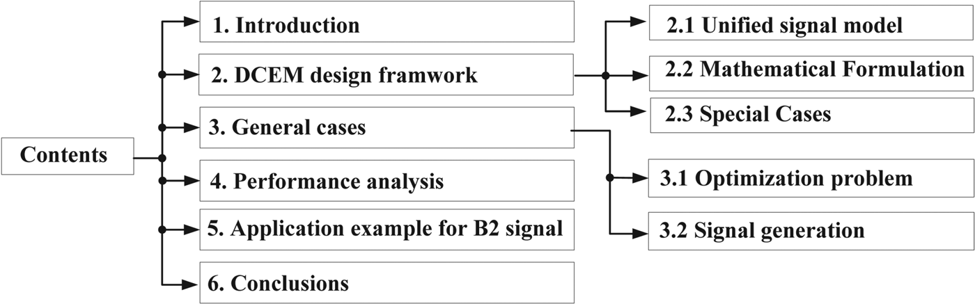
The DCEM methods mentioned above are usually designed for special cases. In this paper, we propose a unified DCEM design framework that allows the unification of existing DCEM methods. The proposed design framework can provide a DCEM scheme for almost all the DCEMs required in GNSS signal design. To be specific, the proposed method converts the DCEM design into an optimisation problem, and thus has no special constraints on the number, power and phase relationship of the signal components. For the desired power and phase relationship, our method can reach higher multiplexing efficiency compared with generalised AltBOC, ACE-BOC and ES ACE-BOC. Figure 1 shows the workflow of this paper. In Section 2, the unified design framework of DCEM is presented, including the signal model and mathematical formulation. ACE-BOC and generalised AltBOC are discussed as special cases of the proposed framework. In Section 3, we analyse the optimisation problem and discuss the signal generation scheme. In Section 4, the performance of the proposed design method is analysed and compared with the existing DCEM methods. In Section 5, we propose a constant envelope multiplexing scheme for the BeiDou B2 signal. Conclusions are summarised in the last section.
The workflow of this paper.

2. DCEM DESIGN FRAMEWORK
DCEM methods can be modelled as a unified framework. AltBOC, ACE-BOC and generalised AltBOC can all be seen as special cases of this unified framework.
2.1. The unified signal model
The proposed unified dual-frequency signal model is as follows. The centre frequency of the lower sideband is −f s, and the centre frequency of the upper sideband is f s. Without loss of generality, we assume that there are L signal components at the lower sideband with L≥0, denoted as vL(t)=[s l,1(t), s l,2(t),···, s l,L(t)]T. There are U signal components at the upper sideband with U≥0, denoted as vU(t)=[s u,1(t), s u,2(t),···, s u,U(t)]T.
Considering that current GNSS signals are usually Binary Phase-Shift Keying (BPSK), BOC or Time-Multiplexed Binary Offset Carrier (TMBOC) modulated signals, all the signal components are binary Pseudo Random Noise (PRN) signals, that is, s l,n(t)∈{1,−1}, 1≤n≤L, s u,m(t)∈{1,−1}, 1≤m≤U, (Yao and Lu, Reference Yao and Lu2013; Guo et al., Reference Guo, Yao and Lu2017). We define  $j=\sqrt{-1}$ as the imaginary unit. P l, n and θl, n are the nominal power and carrier phase of signal component s l, n(t), respectively. P u, m and θu, m are the nominal power and carrier phase of signal component s u, m(t), respectively. S Σ(t) is the direct linear combination of signal components, which is expressed as:
 $$s_{\Sigma} (t) = \sum_{n=1}^L \sqrt{P_{l,n}}e^{j\theta_{l,n}} S_{i,n}(t)e^{-j2\pi f_st} +\sum^U_{m=1} \sqrt{P_{u,m}} e^{j\theta_{u,m}} s_{u,m}(t)e^{j2\pi f_st}$$
The envelope of s Σ(t) is not constant. The purpose of DCEM is to generate a constant envelope composite signal. Moreover, the power, phase and centre frequency of signal components in a DCEM signal should be consistent with those in s Σ(t). In other words, s Σ(t) is the desirable part of the constant envelope composite signal.
Following the method of Huang et al. (Reference Huang, Zhu and Ou2015a; Reference Huang, Zhu, Tang, Gong and Ou2015b), we first exploit the single-frequency constant envelope multiplexing method POCET to separately combine these signal components at the lower sideband and upper sideband into two constant envelope signals. Define s CE, L(t) and s CE, U(t) as the single-frequency constant envelope signals at the lower sideband and upper sideband, respectively. P L and θ L(vL(t)) are the total power and instantaneous phase values of the single-frequency constant envelope signal at the lower sideband, respectively. P U and θ U(vU(t)) are the total power and instantaneous phase values ofthe single-frequency constant envelope signal at the upper sideband, respectively. We have:
 $$s_{{CE},{L}}(t) = \sqrt{P_L}e^{j\theta_L({\bf v}_L(t))}, \quad s_{CE,U}(t) = \sqrt{P_U}e^{j\theta_U({\bf v}_U(t))}$$
It can be seen that a single-frequency constant envelope signal can be equivalent to a phase modulated signal (Dafesh and Cahn, Reference Dafesh and Cahn2009). The phase value is only determined by these values of signal components. Therefore, the different values of θ L(vL(t)) are possibly up to 2L, and the different values of θU are possibly up to 2U. For the sake of simplicity, in the absence of ambiguity, θ L(vL(t)) is denoted as θL, and θ U(vU(t)) is denoted as θU.
Generally speaking, the single-frequency constant envelope composite signal can be written as the sum of the useful signal components and Inter-Modulation (IM) signals (Yan et al., Reference Yan, Tang, Wei, Qu and Zhou2015; Zhang et al., Reference Zhang, Li, Zhou and Wang2012). Define IM L(t) and IM U(t) as the IM terms at the lower sideband and the upper sideband, respectively. Equation (2) is rewritten as:
 $$\eqalign{s_{{CE},{L}}(t) &= \sum_{n=1}^L \sqrt{P_{l,n}}e^{j\theta_{l,n}}s_{l,n}(t)+IM_L(t),\cr s_{{CE},{U}}(t) &= \sum_{m=1}^U \sqrt{P_{u,m}}e^{j\theta_{u,m}}s_{u,m}(t)+IM_U(t)}$$
When L=U=2 and these two signal components at one sideband are orthogonal, we have  $s_{CE,L}(t) = \sqrt{P_{l,1}} s_{l,1}(t) + j \sqrt{P_{l,2}} s_{l,2}(t)$ and
 $s_{CE,U}(t) = \sqrt{P_{u,1}} s_{u,1} (t) + j \sqrt{P_{u,2}} s_{u,2} (t)$. No IM terms are introduced.
Using s CE, L(t) and s CE, U(t) in Equation (2) to replace 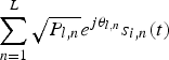 $\sum_{n=1}^{L}\sqrt{P_{l,n}}e^{j\theta_{l,n}}s_{i,n}(t)$ and
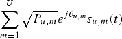 $\sum_{m=1}^{U}\sqrt{P_{u,m}}e^{j\theta_{u,m}}s_{u,m}(t)$ in Equation (1), respectively, the modified linear sum of signal components is written as:
 $$\eqalign{s_{linear}(t) &= s_{CE,L}(t)e^{-j2\pi f_st} + s_{CE,U}(t)e^{j2\pi f_st} = \sqrt{P_L}e^{j\theta_L}e^{-j2\pi f_st} + \sqrt{P_U}e^{j\theta_U}e^{j2\pi f_st} \cr &= \left(\displaystyle{\sqrt{P_L}+\sqrt{P_U} \over 2}\lpar e^{j\theta_L}e^{-j2\pi f_st}+e^{j\theta_U}e^{j2\pi f_st}\rpar \right. \cr &\quad + \left.\displaystyle{\sqrt{P_L}-\sqrt{P_U} \over 2}\lpar e^{j\theta_L}e^{-j2\pi f_st}-e^{j\theta_U}e^{j2\pi f_st}\rpar \right) \cr &=\left(\matrix{\displaystyle{\sqrt{P_U}+\sqrt{P_L} \over 2}e^{j\displaystyle{\theta_U+\theta_L \over 2}}\left(e^{-j\displaystyle{\theta_U+\theta_L \over 2}} e^{-j2\pi f_st}+e^{j\displaystyle{\theta_U-\theta_L \over 2}}e^{j2\pi f_st}\right)\cr -\displaystyle{\sqrt{P_U}+\sqrt{P_L} \over 2}e^{j\displaystyle{\theta_U+\theta_L \over 2}}\left(e^{-j\displaystyle{\theta_U+\theta_L \over 2}} e^{-j2\pi f_st}-e^{j\displaystyle{\theta_U-\theta_L \over 2}}e^{j2\pi f_st}\right)} \right) \cr &=e^{j\displaystyle{\theta_U+\theta_L \over 2}}\left( \matrix{\left(\sqrt{P_U}+\sqrt{P_L}\right)\cos \left(2\pi f_st+\displaystyle{\theta_U-\theta_L \over 2}\right)\cr +j\left(\sqrt{P_U}+\sqrt{P_L}\right)\sin \left(2\pi f_st+\displaystyle{\theta_U-\theta_L \over 2}\right)}\right) \cr &= e^{j\displaystyle{\theta_U+\theta_L \over 2}}s_{linear,0}\left(t+\displaystyle{\theta_U-\theta_L \over 4\pi f_s}\right)}$$
where s linear,0(t) is defined by:
 $$s_{linear,0}(t)=\left(\sqrt{P_U}+\sqrt{P_L}\right)\cos (2\pi f_st)+j\left(\sqrt{P_U}+\sqrt{P_L}\right)\sin (2\pi f_st)$$
When P L=P U, the trajectory of s linear,0(t) is a line in the complex plane. When P L≠P U, the trajectory of s linear,0(t) is an ellipse with the semi-major axis 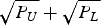 $\sqrt{P_{U}}+\sqrt{P_{L}}$ and eccentricity
 $2\,{^{4}\!\!\!\sqrt{P_{L}P_{U}}}/(P_{U}+P_{L})$. For different combinations of θL and θU, the trajectory of s linear(t) only rotates (θ U+θ L)/2 degrees along the counter clockwise direction, and the initial time changes to (θ U−θ L)/(4πf s).
2.2. Mathematical formulation
In Equation (5), s linear,0(t) is a periodic signal with period T s=1/f s. However, the envelope of s linear,0(t) is not constant. To achieve constant envelope multiplexing, we reconstruct a constant envelope periodic signal sc(t) with period T s. Each period of sc(t) is sub-divided in M equal sub-periods, M is an even number. Then sc(t) is expressed as:
 $$sc(t)=A\sum_{i=0}^{M-1} e^{j\varphi_i} p\left(t-\displaystyle{iT_s \over M}\right),\quad 0 \leq t \lt T_s$$
where p(t) is the rectangular function which is unity from 0≤t<T s/M and zero elsewhere. Considering that the real part of s linear,0(t) is an even function, and the imaginary part of s linear,0(t) is an odd function, we let φi=−φM−i−1, 0≤i<M. Only M/2 phase values are required. In Section 3, for a certain M, A and {φi} can be solved by the optimisation process to reach the optimal multiplexing efficiency. Therefore, sc(t) is uniquely determined by M.
We expand the real part and imaginary part of sc(t) into the Fourier series expression and define a p, cos as the pth order Fourier coefficients of cosine terms. a q, sin is the qth order Fourier coefficients of sine terms. The Fourier series expression of sc(t) is:
 $$sc(t) = A\sum_{p=0}^{\infty} a_{p,\cos} \cos (2\pi pf_s t) + j\sum_{q=1}^{\infty} a_{q,\sin} \sin (2\pi qf_s t)$$
where the coefficients of the Fourier series can be calculated by:
 $$\eqalign{a_{0,\cos} &= \displaystyle{1 \over T_s} \int^{T_s}_0 \hbox{Re}(sc(t))dt = A\sum^{M-1}_{i = 0}\cos \varphi_i \cr a_{p,\cos} &=\displaystyle{2 \over T_s} \int^{T_s}_0 \hbox{Re}(sc(t)) \cos (2p\pi f_s t)dt, p \gt 0 \cr a_{q,\sin} &= \displaystyle{2 \over T_s}\int^{T_s}_0 \hbox{Im}(sc(t))\sin(2q\pi f_st)dt, q \gt 0}$$
In order to maintain an unchanged power and phase relationship between signal components, neglecting the high-order harmonic components of sc(t), the fundamental frequency components of sc(t) have to be fully equal to s linear,0(t). Comparing Equation (7) with Equation (5), we have
 $$\eqalign{a_{0,\cos} &= \sum^{M-1}_{i=0} \cos \theta_i = 0 \cr a_{1,\cos} &= \sum^{M-1}_{i = 0}\displaystyle{2A\cos \theta_i \over \pi} \sin \displaystyle{\pi \over M} \cos \displaystyle{2\pi i + \pi \over M} = \sqrt{P_U} + \sqrt{P_L} \cr a_{1,\sin} &= \sum^{M-1}_{i = 0} \displaystyle{2A \sin \theta_i \over \pi} \sin \displaystyle{\pi \over M} \sin \displaystyle{2\pi i + \pi \over M} = \sqrt{P_U} - \sqrt{P_L}}$$
We define H(t) as the sum of high-order harmonic components in sc(t), that is,
 $$H(t)= \sum_{p=2}^{\infty} \lpar a_{p,\cos} \cos(2\pi pf_s t)\rpar + j\sum_{q=2}^{\infty} \lpar a_{q,\sin} \sin(2\pi qf_s t)\rpar $$
Thus, sc(t)=s linear,0(t)+H(t). Define s CE(t) as the DCEM signal. Using the s CE(t) and sc(t) to replace s linear(t) and s linear,0(t) in Equation (4), respectively, we have:
 $$\eqalign{s_{CE}(t)&=e^{j\displaystyle{\theta_L+\theta_U \over 2}}sc\left(t+\displaystyle{\theta_U-\theta_L \over 4\pi f_s}\right) =e^{j\displaystyle{\theta_L+\theta_U \over 2}}\left(s_{linear,0}\left(t+\displaystyle{\theta_U-\theta_L \over 4\pi f_s}\right)+H\left(t+\displaystyle{\theta_U-\theta_L \over 4\pi f_s}\right)\right) \cr &=e^{j\displaystyle{\theta_L+\theta_U \over 2}}s_{linear,0}\left(t+\displaystyle{\theta_U-\theta_L \over 4\pi f_s}\right) +e^{j\displaystyle{\theta_L+\theta_U \over 2}}H\left(t+\displaystyle{\theta_U-\theta_L \over 4\pi f_s}\right) \cr &=s_{linear}(t)+e^{j\displaystyle{\theta_L+\theta_U \over 2}}H\left(t+\displaystyle{\theta_U-\theta_L \over 4\pi f_s}\right)}$$
Substituting Equations (3) and (4) into Equation (10), we can obtain:
 $$\eqalign{s_{CE}(t)&=s_{CE,L}(t)e^{-j2\pi f_{s}t}+s_{CE,U}e^{j2\pi f_{s}t}+e^{j\displaystyle{\theta_{L}+\theta_{U} \over 2}}H\left(t+\displaystyle{\theta_{U}-\theta_{L} \over 4\pi f_{s}}\right) \cr &=\left(\sum_{n=1}^{L}\sqrt{P_{l,n}}e^{j\theta_{l,n}}s_{l,n}+IM_{L}(t)\right)e^{-j2z\pi f_{s}t}+\left(\sum_{m=1}^{U}\sqrt{P_{u,m}}e^{j\theta_{u,m}}s_{u,m}+IM_{U}(t)\right)e^{j2\pi f_{s}t}\cr &\quad +e^{j\displaystyle{\theta_{L}+\theta_{U} \over 2}}H\left(t+\displaystyle{\theta_{U}-\theta_{L} \over 4\pi f_{s}}\right) \cr &=s_{\Sigma}(t)+IM_{L}(t)e^{-j2\pi f_{s}t}+IM_{U}(t)e^{j2\pi f_{s}t}+\overline{H}(t)}$$
where  $\overline{H}(t)$ denotes the high-order harmonic components in s CE(t), which is given by:
 $$\overline{H}(t)=e^{j\displaystyle{\theta_{L}+\theta_{U} \over 2}}H\left(t + \displaystyle{\theta_{U} - \theta_{L} \over 4\pi f_{s}} \right)$$
Equation (11) shows that s CE(t) is composed of the linear combination of useful signal components, IM terms and high-order harmonic components.
2.3. Special cases
Theoretically, we can generate different reconstructed signals sc(t) to satisfy Equation (9). In fact, AltBOC, generalised AltBOC and ACE-BOC can be seen as the special cases of the proposed unified DCEM method. They are applied for the following case.
 $$\matrix{L = 2, U = 2 \cr \theta_{l,1} = 0, \theta_{l,2} = \displaystyle{\pi \over 2}, \theta_{u,1} = 0, \theta_{u,2} = \displaystyle{\pi \over 2}}$$
In ACE-BOC, these four signal components can have arbitrary power allocation. AltBOC is a special case of ACE-BOC in which four signal components have equal power. ACE-BOC is obtained by (Yao and Lu, Reference Yao and Lu2013):
 $$s_{ACE-BOC} (t) = \hbox{sign}(\hbox{Re}(s_{\Sigma}(t))) + j\hbox{sign} (\hbox{Im}(s_{\Sigma}(t)))$$
where sign(·) is the signum function. Re(x) represents the real part of x, and Im(x) is the imaginary part of x. Thus, the reconstructed signal in ACE-BOC is calculated by:
 $$\eqalign{sc_{ACE-BOC}(t) &=\hbox{sign}(\hbox{Re}(s_{linear,0}(t)))+j\hbox{sign}(\hbox{Im}(s_{linear,0}(t))) \cr &=\left(\sqrt{P_{U}}+\sqrt{P_{L}}\right)\hbox{sign}(\cos(2\pi f_{s}t))+j\left(\sqrt{P_{U}}-\sqrt{P_{L}}\right)\hbox{sign}(\sin(2\pi f_{s}t))}$$
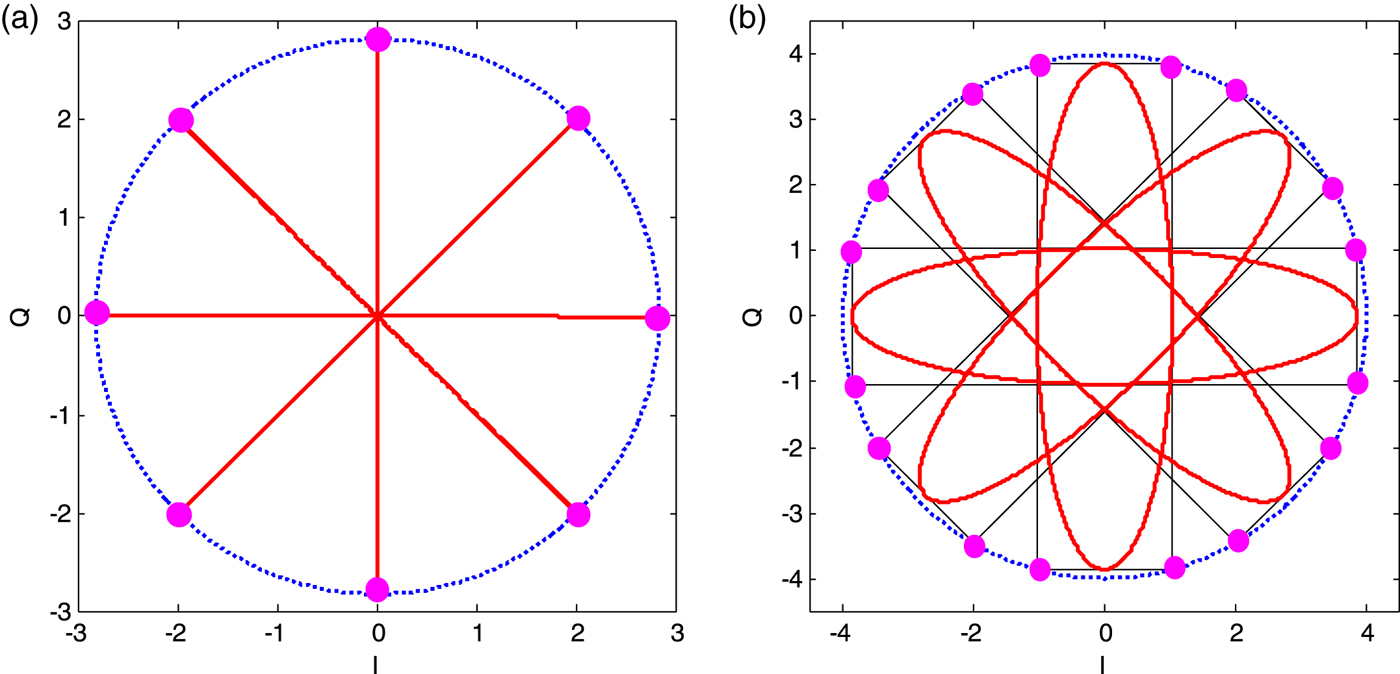
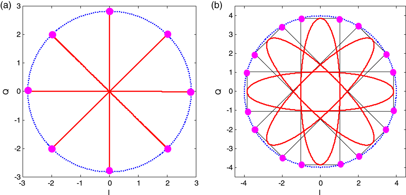
Each period of sc ACE−BOC(t) in ACE-BOC is sub-divided in four equal sub-periods. Figure 2 shows how to reconstruct the linear sum s linear(t) into a constant envelope signal in ACE-BOC. The trajectory and modulation constellation of AltBOC and ACE-BOC are presented in detail. In Figure 2(b), the power ratio of four signal components P l,1, P l,2, P u,1 and P u, 2 is 1: 1:3:3.
The trajectory and modulation constellation. (a) AltBOC (b) ACE-BOC.
In generalised AltBOC, the power of four signal components P l,1, P l,2, P u,1 and P u, 2 satisfy the following requirements, that is, P l,2=P l,1, P u,2=P u,1 and P u,1/P l,1=β 2. The expression of generalised AltBOC is given by:
 $$s_{{\rm generalised\ AltBOC}}(t)= \left(\matrix{(s_{l,1}(t)+js_{l,2}(t))e^{-j^{\displaystyle{\pi \over 8}k_{s}(t)}}+\beta(s_{u,1}(t)+js_{u,2}(t))e^{j^{\displaystyle{\pi \over 8}k_{s}(t)}}\cr +b(s_{aI}(t)+js_{aQ}(t))e^{j^{\displaystyle{\pi \over 8}k_{p}(t)}}+a(s_{bI}(t)+js_{bQ}(t))e^{-j\displaystyle{\pi \over 8}k_{p}(t)}}\right)$$
where s aI(t)=s l,2 (t) s u,1 (t) s u,2 (t), s aQ(t)=s l,2(t)s u,1(t)s u,2(t), s bI (t)=s l,1 (t)s l,2 (t)s u,2 (t) and s bQ(t)=s l,1(t)s l,2(t)s u,1(t). k s(t) and k p(t) are listed in Table 1. Parameters a and b depend on the value of β, and their relationship has been derived by Zhang et al. (Reference Zhang, Zhou and Wang2013).
The values of k s(t) and k p(t).

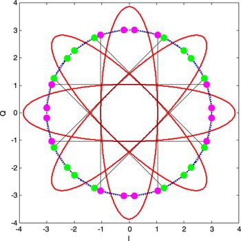
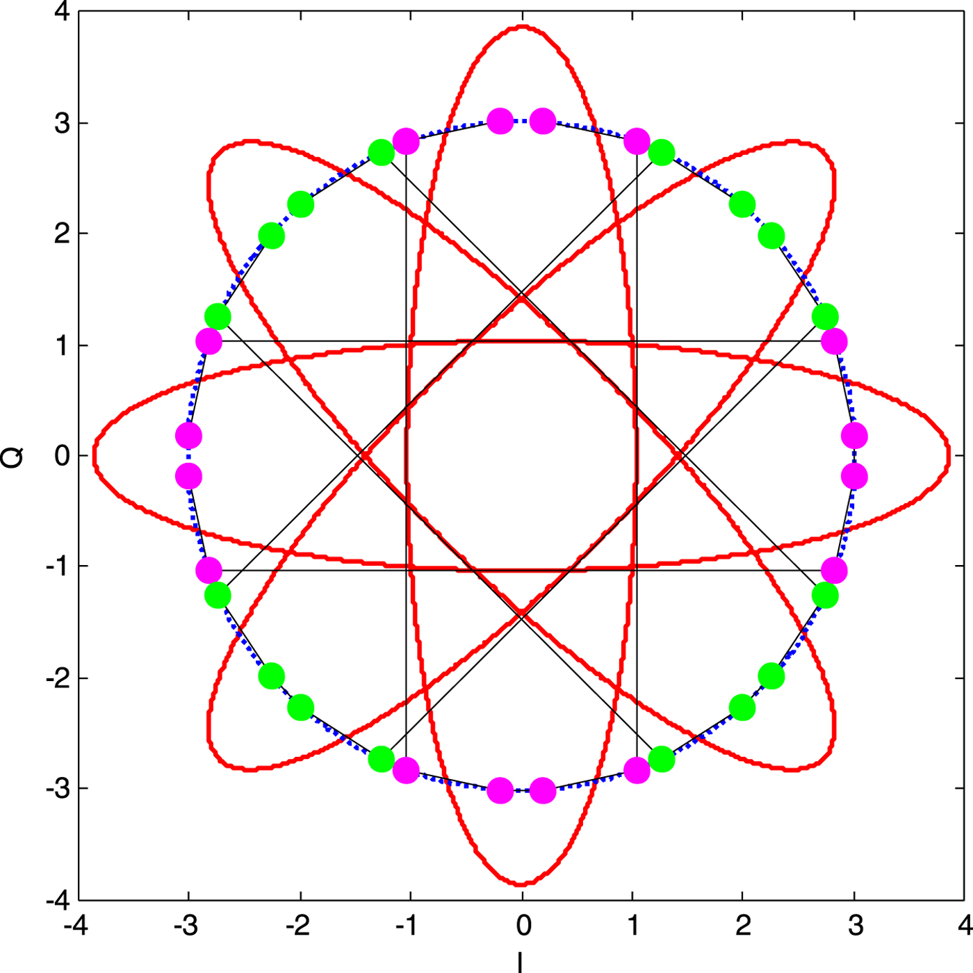
Each subcarrier period is sub-divided in M=8 equal sub-periods in generalised AltBOC. As shown in Figure 3, for different combinations of θU and θL, each ellipse is mapped to eight phase points in one circle. In Figures 2 and 3, the radius of the circle represents the envelope value A. The total transmission power is A 2. The multiplexing efficiency is defined by the ratio between the power of all the useful signal components and the total transmission power (Fan et al., Reference Fan, Lin, Wang and Dafesh2008). The configurations in Figure 3 and Figure 2(b) have the same power as all the useful signal components. However, the required total transmission power of generalised AltBOC is obviously less than that of ACE-BOC, which implies that the multiplexing efficiency of generalised AltBOC is higher than that of ACE-BOC.
The trajectory and modulation constellation of generalised AltBOC with β2=3.
3. THE GENERAL CASE
For the general case, the reconstructed signal sc(t) can be obtained by solving Equation (9). Among these solutions, it is expected that the multiplexing efficiency is as high as possible. The design of DCEM can now be converted into an optimisation problem.
3.1. The optimisation problem
The multiplexing efficiency is the ratio between the power of all the useful signal components and the total transmission power. Defining 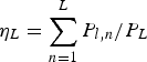 $\eta_{L}=\sum_{n=1}^{L}P_{l,n}/P_{L}$ and
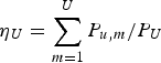 $\eta_{U}=\sum_{m=1}^{U}P_{u,m}/P_{U}$ as the single-frequency constant envelope multiplexing efficiency of the lower sideband and upper sideband, respectively, then η is the total multiplexing efficiency of the DCEM signal. For the unified DCEM signal model, the multiplexing efficiency η is given by:
 $$\eta = \displaystyle{\sum_{n=1}^{L}P_{l,n}+\sum_{m=1}^{U}P_{u,m} \over A^{2}}=\displaystyle{P_{L}\cdot\eta_{L}+P_{U}\cdot\eta_{U} \over A^{2}}$$
To maximise η is equivalent to minimising the envelope value A. For a certain M, Equation (9) shows the constraint conditions. The nonlinear optimisation problem is expressed as:
 $$\eqalign{&\quad \min \quad A^2 \hfill \cr & s.t.\left\{\matrix{\varphi_i = -\varphi_{M-1-i} \hfill \cr \sum\limits_{i=0}^{M-1}\displaystyle{2A\cos\varphi_i \over \pi}\sin\displaystyle{\pi \over M}\cos\displaystyle{2\pi i+\pi \over M}=\sqrt{P_U}+\sqrt{P_L} \hfill \cr \sum\limits_{i=0}^{M-1}\displaystyle{2A\sin\varphi_i \over \pi}\sin\displaystyle{\pi \over M}\sin\displaystyle{2\pi i+\pi \over M}=\sqrt{P_U}-\sqrt{P_L} \hfill \cr \sum\limits_{i=0}^{M-1}\cos \varphi_i=0 \hfill}\right.}$$
The values of A and {φi, 0≤i<M} can be obtained by solving Equation (18). For certain values of P U and P L, these values depend only on M. It is difficult to solve the analytical solution of Equation (18). We can obtain the optimal solution based on a numerical optimisation algorithm for general cases. Equation (18) is a constrained nonlinear optimisation problem. Usually, Equation (18) can be equivalent to an unconstrained optimisation problem by using the positive penalty function method (Dafesh and Cahn, Reference Dafesh and Cahn2009; Yan et al., Reference Yan, Wei, Tang and Zhou2016), that is:
 $$\min \ A^{2} + \mu_{a} \left(\matrix{\left(\sum\limits_{i=0}^{M-1}\displaystyle{2A\cos\varphi_{i} \over \pi}\sin\displaystyle{\pi \over M}\cos\displaystyle{2\pi i+\pi \over M} - \left(\sqrt{P_{U}}+\sqrt{P_{L}}\right)\right)^{2} \hfill \cr +\left(\sum\limits_{i=0}^{M-1}\displaystyle{2A\sin\varphi_{i} \over \pi}\sin\displaystyle{\pi \over M}\sin\displaystyle{2\pi i+\pi \over M} - \left(\sqrt{P_{U}}-\sqrt{P_{L}}\right)\right)^{2} \hfill \cr +\left(\sum\limits_{i=0}^{M-1}\cos\varphi_{i}\right)^{2} \hfill}\right)$$
where μa is the positive penalty factor. Then the optimal numerical solution can be found through some existing optimisation algorithms, such as the quasi-Newton method (Jasbir Reference Jasbir2004). Considering φi=−φM−1−i, there are only M/2 phases needing to be determined.
For some special cases, it is possible to derive an analytical solution of Equation (18). For example, when P U=P L, we have 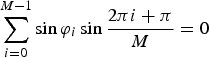 $\sum_{i = 0}^{M - 1} \sin \varphi_{i} \sin \displaystyle{2\pi i + \pi \over M} = 0$ according to Equation (18). In this case, in order to simplify Equation (18), we consider an unnecessary and sufficient condition, such as, sinφi=0 for all i. Note here that we use a stronger constraint, and intentionally narrow the range of possible solutions. Then we derive that
 $\varphi_{i}\in \{0,\ \pi\}$, and cosφi∈{1,−1}. It is thus easy to verify that the third constraint condition in Equation (18) is established.
According to the second constraint condition in Equation (18), the envelope A is expressed as:
 $$A = \displaystyle{\sqrt{P_{U}}+\sqrt{P_{L}} \over \sum_{i=0}^{M-1}\displaystyle{2\cos\varphi_{i} \over \pi}\sin\displaystyle{\pi \over M}\cos\displaystyle{2\pi i+\pi \over M}}=\displaystyle{\sqrt{P_{U}}+\sqrt{P_{L}} \over \displaystyle{2 \over \pi}\sin\displaystyle{\pi \over M}\sum_{i=0}^{M-1}\cos\varphi_{i}\cos\displaystyle{2\pi i+\pi \over M}}$$
The objective minimising A 2 is equivalent to maximising 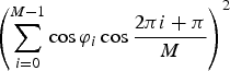 $\left(\sum_{i=0}^{M-1} \cos \varphi_{i} \cos \displaystyle{2\pi i+\pi \over M}\right)^{2}$. Equation (18) is rewritten as:
 $$\eqalign{\max &\left(\sum_{i = 0}^{M-1} \cos \varphi_{i} \cos \displaystyle{2\pi i+\pi \over M}\right)^{2}\cr s.t. &\left\{\matrix{\cos\varphi_{i}=\cos\varphi_{M-1-i} \hfill \cr \sum_{i=0}^{M-1}\cos\varphi_{i}=0 \hfill \cr \cos\varphi_{i}\in \{1,-1\} \hfill}\right.}$$
Since cosφi∈{1,−1}, thus  $\sum_{i=0}^{M-1}\cos\varphi_{i}\cos\displaystyle{2\pi i+\pi \over M}\leq\sum_{i=0}^{M-1}\vert \cos\varphi_{i}\vert \left\vert \cos\displaystyle{2\pi i+\pi \over M}\right\vert = \sum_{i=0}^{M-1} \left\vert \cos\displaystyle{2\pi i+\pi \over M}\right\vert$. The equality can hold only when the following condition is satisfied:
 $$\cos \varphi_{i} = \hbox{sign}\left(\cos \displaystyle{2\pi i+\pi \over M} \right) \hbox{for all} i$$
Equation (20) requires that M should be a multiple of four. Then we can obtain a special solution Equation (18) for P U=P L, that is:
 $$\eqalign{\varphi_{i}&=\arccos \left(\hbox{sign}\left(\cos\displaystyle{2\pi i+\pi \over M}\right)\right),i=0,1,\hbox{L},M-1\cr A&=\displaystyle{\sqrt{P_{U}}+\sqrt{P_{L}} \over \sum_{i=0}^{M-1}\displaystyle{2\cos\varphi_{i} \over \pi}\sin\displaystyle{\pi \over M}\cos\displaystyle{2\pi i+\pi \over M}} = \displaystyle{\pi\left(\sqrt{P_{U}}+\sqrt{P_{L}}\right) \over 2\sin\displaystyle{\pi \over M}\sum_{i=0}^{M-1} \left\vert \cos\displaystyle{2\pi i+\pi \over M}\right\vert }\cr &=\displaystyle{\pi \left(\sqrt{P_{U}}+\sqrt{P_{L}}\right) \over 8\sin\displaystyle{\pi \over M}\sum_{i=0}^{M/4-1}\cos\displaystyle{2\pi i+\pi \over M}} = \displaystyle{\pi\left(\sqrt{P_{U}}+\sqrt{P_{L}}\right) \over 4} = \displaystyle{\pi \over 2}\sqrt{P_{U}}}$$
When M is a multiple of four, the above solution can achieve the optimal multiplexing efficiency in the case of P U=P L. According to Equation (17), the multiplexing efficiencyis  $\eta = \displaystyle{P_{L}\cdot \eta_{L} + P_{U}\cdot \eta_{U} \over A^{2}} = \displaystyle{4(\eta_{L}+\eta_{U}) \over \pi^{2}P_{U}}P_{U} = \displaystyle{\eta_{L}+\eta_{U} \over 2}\times 81{\cdot}06\%$. In fact, the optimalsolution is exactly ACE-BOC and GCE-BOC (Huang et al., Reference Huang, Zhu and Ou2015a; Reference Huang, Zhu, Tang, Gong and Ou2015b) in this case. We should keep in mind that Equation (19) still has solutions when M is not a multiple of four. However, the multiplexing efficiency would be relatively lower.
3.2. Signal generation
After solving for A and {φi}, we can generate sc(t). According to Equation (10), the DCEM signal is expressed as:
 $$s_{CE}(t)=e^{j\displaystyle{\theta_{L}+\theta_{U} \over 2}}sc\left(t+\displaystyle{\theta_{U}-\theta_{L} \over 4\pi f_{s}}\right) = Ae^{j\theta_{CE}(t)}$$
where θ CE(t) is the instantaneous phase of s CE(t), which is expressed as:
 $$\theta_{CE}(t) = \displaystyle{\theta_{U}({\bf v}_{U}(t))+\theta_{L}({\bf v}_{L}(t)) \over 2} + \varphi\left\lfloor \hbox{mod} \left(\left\lfloor \displaystyle{Mt \over T_{s}}+\displaystyle{M(\theta_{U}({\bf v}_{U}(t))-\theta_{L}({\bf v}_{L}(t))) \over 4\pi}\right\rfloor, M \right)\right\rfloor$$
where  $\lfloor \cdot \rfloor$ is the floor integral function. θ U(vU(t)) has at most 2U values, θ L(vL(t)) has at most 2L values and {φi} has M phase values. Therefore, θ CE(t) has at most M×2L+U values.
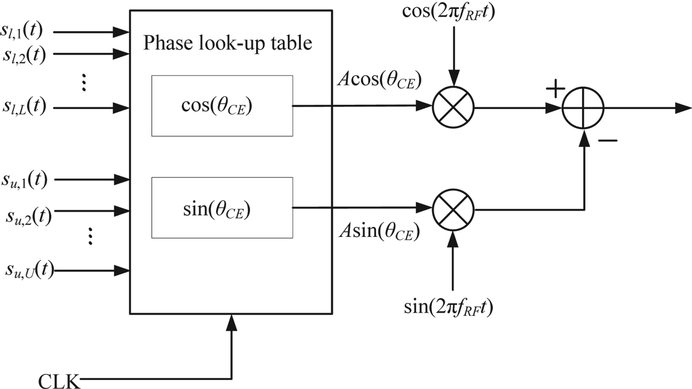
The DCEM signal s CE(t) can be generated based on a pre-stored two-dimensional phase Look-Up Table (LUT) according to Equation (22), which is similar to the AltBOC signal (OS SIS ICD, 2016). Figure 4 shows the generation scheme of the proposed DCEM signal. In Figure 4, f RF denotes the carrier frequency and CLK represents the sampling clock. Time t can be determined by the clock rate f CLK.
Implementation of the proposed DCEM signal.

In a real situation, the clock rate f CLK should be limited. We can derive the minimum clock rate to generate s CE(t) according to Equation (22). Assume that there are in total K possible values for θ U(vU(t))−θ L(vL(t))≠0, 0<K≤2L+U. For these K values, we denote:
 $$\left\vert \displaystyle{\theta_{U}({\bf v}_{U}(t)) - \theta_{L}({\bf v}_{L}(t)) \over 4\pi}\right\vert = \displaystyle{q_{k} \over r_{k}}, k = 1,2, \cdots\, K$$
where 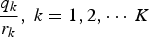 $\displaystyle{q_{k} \over r_{k}},\ k = 1,2, \cdots\, K$ are the fractions in lowest terms, that is, the greatest common divisor of r k and q k is one. Denote the minimum common multiple of M and {r k, k=1, 2,···K} is M min. Then the required minimum clock rate f CLK=M minf s. Clearly, f CLK≥Mf s.
When the clock rate  $f_{CLK} = M_{min}f_{s}, \theta_{CE}(t)$ is constant during any time interval t mod T s∈[iT s/M min, (i+1)T s/M min), i=0, 1,···M min−1. Then the DCEM signal can be generated using the pre-stored M min×2L+U two-dimensional phase LUT. It is easy to verify that if for any values of θ L(vL(t)) and θ U(vU(t)), M(θ U−θ L)/(4π) is an integer, the minimum clock rate would be f CLK=Mf s.
For clarity, considering the previous example, that is, L=2, U=2, θ l,1=0,  $\theta_{l,2} = \displaystyle{\pi \over 2}$. θ u,1=0,
 $\theta_{u,2}=\displaystyle{\pi \over 2}$, P l,2=P l,1=1, P u,2=P u,1=3. We have
 $\theta_{U}({\bf v}_{U}(t))\in \left\{\displaystyle{\pi \over 4}, \displaystyle{3\pi \over 4},\displaystyle{5\pi \over 4},\displaystyle{7\pi \over 4}\right\}$ and
 $\theta_{L}({\bf v}_{L}(t))\in \left\{\displaystyle{\pi \over 4}, \displaystyle{3\pi \over 4},\displaystyle{5\pi \over 4},\displaystyle{7\pi \over 4}\right\}$. Thus,
 $\left\vert \displaystyle{\theta_{U}({\bf v}_{U}(t))-\theta_{L}({\bf v}_{L}(t)) \over 4\pi}\right\vert \in \left\{\displaystyle{1 \over 8}, \displaystyle{1 \over 4}, \displaystyle{3 \over 8}\right\}$ when
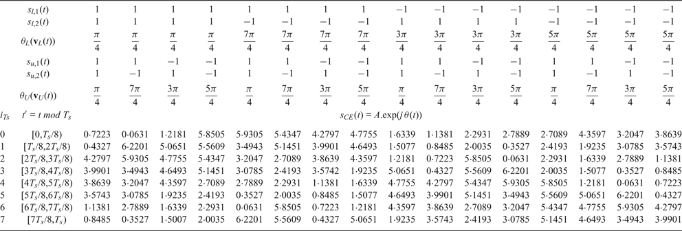
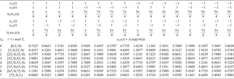
 $\theta_{U}({\bf v}_{U}(t))-\theta_{L}({\bf v}_{L}(t))\ \ne 0$. Set M=8, then the required minimum clock rate f CLK=8f s. The size of the two-dimensional phase LUT is 8×16. Based on the Matlab platform, the quasi-Newton method can be achieved to solve Equation (18), then we have:
 $$\eqalign{\varphi_{0} &= -0.0631,\varphi_{1} = -0.3572,\varphi_{1}=3.4943,\varphi_{4}=3.2047\cr \varphi_{5}&=-3.2047,\varphi_{6}=-3.4943,\varphi_{7}=0.3572,\varphi_{8}=0.0631\cr A &= 2.1883}$$
Substituting the values of {φi, i=0, 1, 2,···, 7} into Equation (22), the phase values in the two-dimensional phase LUT can be obtained, as shown in Table 2. In fact, this example is equivalent to generalised AltBOC. The modulation constellation can be found in Figure 3.
Example of two-dimensional phase LUT.
4. PERFORMANCE ANALYSIS
The DCEM signal in a GNSS is mainly a dual-frequency case with four signal components, such as AltBOC (Lestarquit et al., Reference Lestarquit, Artaud and Issler2008), generalised AltBOC (Zhang et al., Reference Zhang, Zhou and Wang2013), ACE-BOC (Yao and Lu, Reference Yao and Lu2013) and ES ACE-BOC (Yao et al., Reference Yao, Zhang and Lu2016). In this section, several typical power allocation schemes proposed in Yao et al. (Reference Yao, Zhang and Lu2016) are used to analyse the performance. Here, we have
 $$\eqalign{s_{CE,L}(t) &= \sqrt{P_{l,1}}s_{l,1}(t)+j\sqrt{P_{l,2}}s_{l,2}(t),\eta_{L} = 1 \cr s_{CE,U}(t) &= \sqrt{P_{u,1}}s_{u,1}(t) + j\sqrt{P_{u,2}}s_{u,2}(t), \eta_{U} = 1}$$
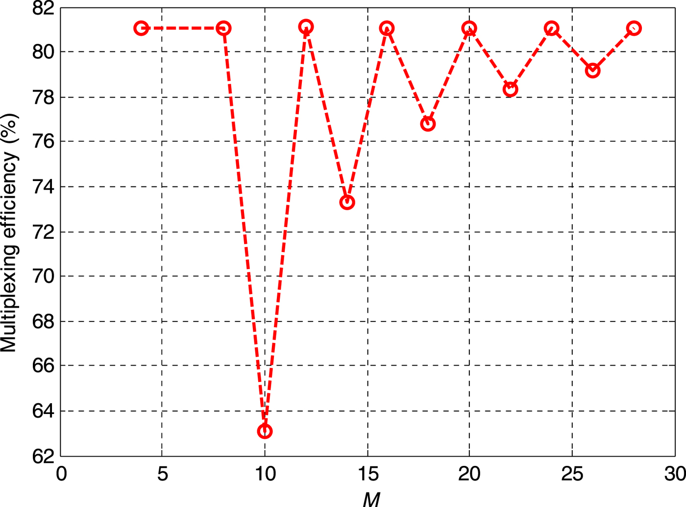
The first power allocation scheme is P u,2=P l,2=β 2P u,1=β 2P l,1. In this case, the lower sideband and upper sideband have equal power, that is, P U=P L. Figure 5 shows the optimal multiplexing efficiency by solving Equation (18) for different M.
Multiplexing efficiency versus M with P U=P L.
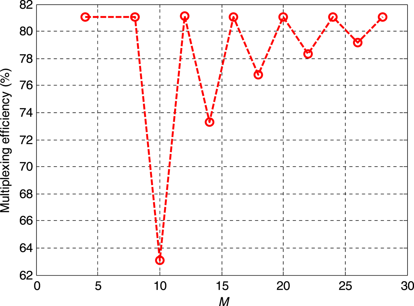
It can be seen that the optimal multiplexing efficiency is 81·06% when M is the integer times four, which is consistent with the previous analysis.
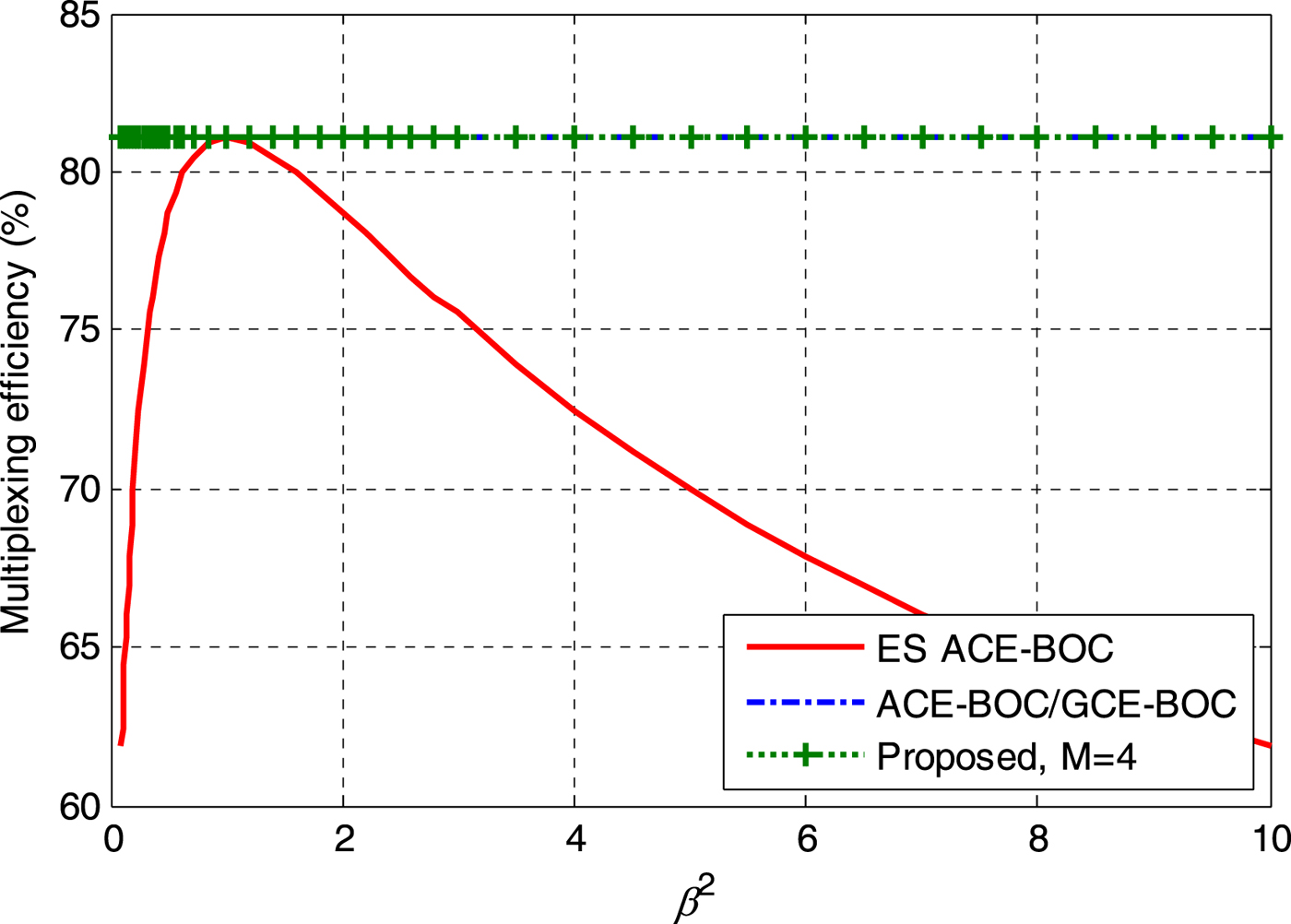
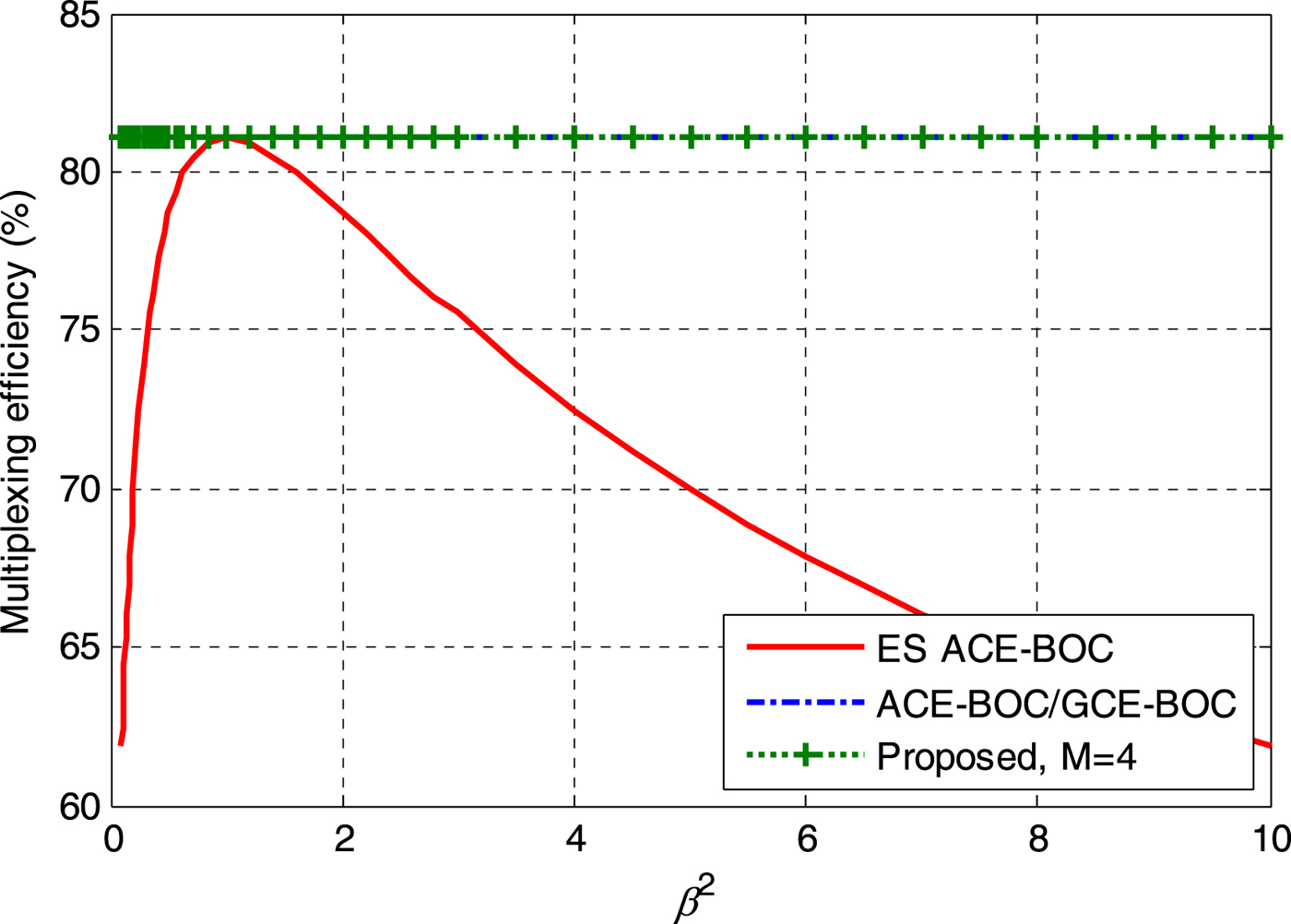
Figure 6 shows the multiplexing efficiencies of ES ACE-BOC, ACE-BOC and the proposed method (M=4) for different β2. Due to ηL=1 and ηU=1, for a certain M, the multiplexing efficiency of the proposed method is unchanged with β, which is the same as ACE-BOC, and higher than ES ACE-BOC. It can be noted that ACE-BOC can be seen as a special case of GCE-BOC, and they have the same multiplexing efficiency for this case.
Multiplexing efficiency versus β2.
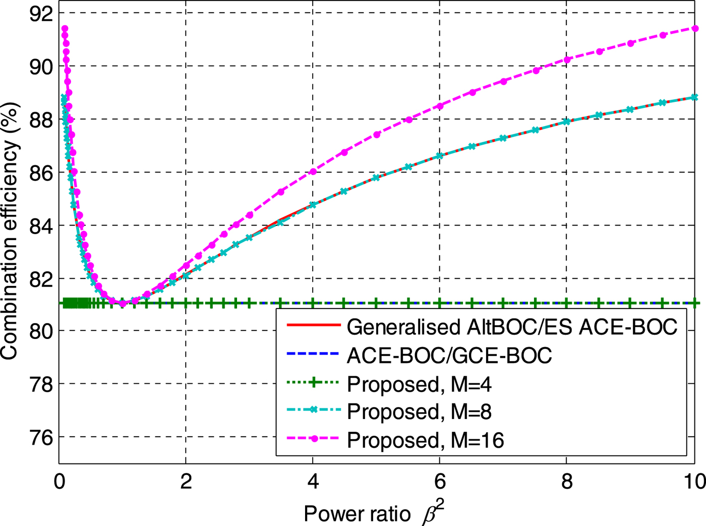
The second power allocation scheme is P u,2=P u,1=β 2P l,2=β 2P l,1, that is, P U/P L=β 2. Figure 7 presents the multiplexing efficiencies in this case for different β2. It can be observed that the multiplexing efficiency of the proposed method is the same as that of ACE-BOC when M=4. When M=8, the multiplexing efficiency of the proposed method is the same as that of generalised AltBOC and ES ACE-BOC. When M increases to 16, the proposed method can reach a higher multiplexing efficiency than that of other methods. Moreover, it should be noted that when M=8 and 16, the greater the power difference between P U and P L, the higher the multiplexing efficiency.
Multiplexing efficiency versus P U/P L.
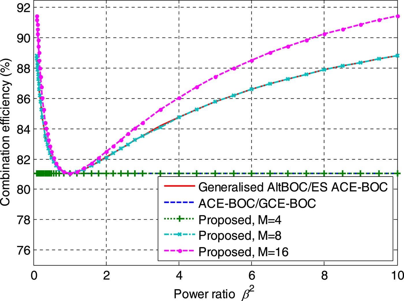
It can be seen from the above analysis that the proposed method can reach higher multiplexing efficiency compared with generalised AltBOC, ACE-BOC (GCE-BOC) and ES ACE-BOC. Moreover, when M=4, ACE-BOC can be obtained with the proposed method. When M=8, the generalised AltBOC can be obtained with the proposed method.
The total transmission power of a constant envelope multiplexing signal is limited. The multiplex efficiency has a significant impact on the effective power of each signal component. Higher multiplexing efficiency means more useful power for each signal component, and the code tracking accuracy can thus be improved. In particular, when the multiplexing efficiency is increased by 10% (for example, from 71·06% to 81·06%), the useful power of each signal component has an improvement of 0·57dB (10lg (81·06/71·06)). Table 3 lists the code tracking error of a BPSK(10) signal with different multiplexing efficiencies. C/N 0 denotes the carrier-to-noise-density ratio with multiplexing efficiency 71·06%. The expression of code tracking error has been provided by Sleewaegen and Wilde (Reference Sleewaegen and Wilde2004). In the calculation, the correlator spacing is one chip, the code loop noise bandwidth is 1 Hz, and the coherent integration time is 1 ms. It can be seen that when C/N 0=25dB-Hz, the code tracking accuracy would have an improvement of 0·37 m when the multiplexing efficiency increases to 81·06%.
Code tracking error with different multiplexing efficiencies.

5. APPLICATION EXAMPLE FOR B2 SIGNAL
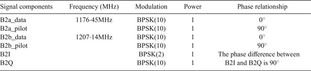
There exist B2I and B2Q signals at the B2 frequency in the BeiDou regional system, which are a QPSK modulation (Montenbruck et al., Reference Montenbruck, Hauschild, Steigenberger, Hugentobler, Teunissen and Nakamura2013). For the BeiDou global system, there are two open service signals, B2a and B2b. Both B2a and B2b include a data component and a pilot component (Tang et al., Reference Tang, Zhou, Hu, Liu and Zhou2010), which form a QPSK(10) modulation. Based on the proposed method, we provide a scheme to combine the regional and global signals at the B2 frequency into a constant envelope signal. The signal parameters of B2 signal are listed in Table 4.
The signal parameters of the B2 signal.

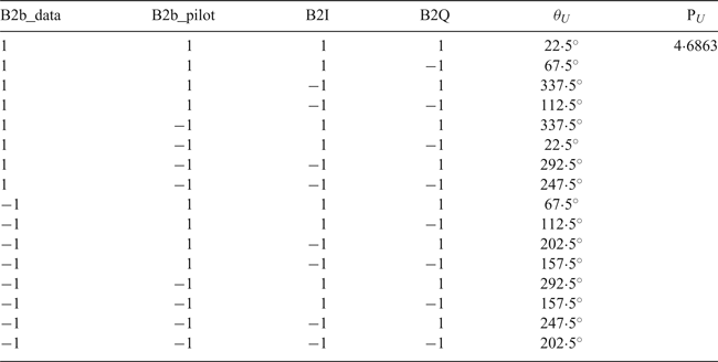
In this case, the subcarrier frequency f s=15·345 MHz. Firstly, the signal components at each sideband are combined separately into two constant envelope signals using single-frequency constant envelope multiplexing. Tables 5 and 6 give the LUTs of the lower and upper sideband, respectively. Here, P L=2, ηL=1, P U=4·6863, η U=85·3553%. The phase values of B2b_data, B2b_pilot, B2I and B2Q are 0°, 90°, 45° and 135°.
The LUT for the constant envelope signal at lower sideband.

The LUT for the constant envelope signal at lower sideband.

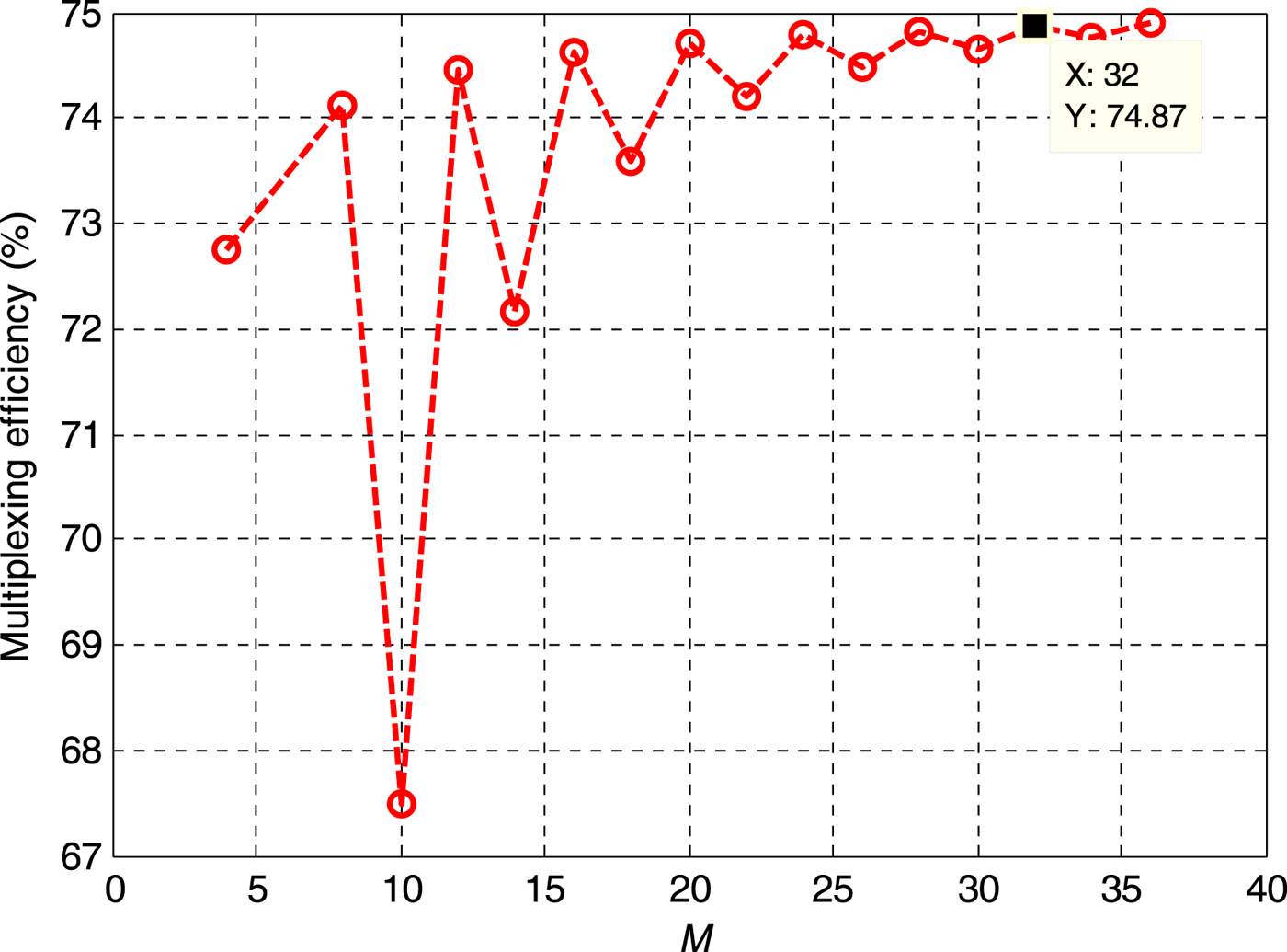
For different values of M, by solving Equation (18), the envelope value A of the dual-frequency constant envelope signal can be obtained. Then the multiplexing efficiency can be calculated by Equation (17). Figure 8 shows the multiplexing efficiency of the B2 signal with the proposed method. Similar to the results in Figure 5, when M is the integer times four, the multiplexing efficiency is relatively higher.
Multiplexing efficiency versus M for B2 signal.
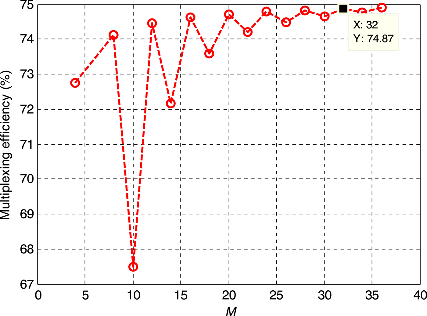
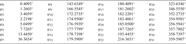
When M=32, the multiplexing efficiency is 74·87%. The required minimum clock rate f CLK=32f s=491·04MHz, which is higher than that of AltBOC. The size of the two-dimensional phase LUT is 32×64. {φi, i=0, 1,···, 31} can be obtained by solving Equation (18), and the results are listed in Table 7.
The optimised results of#lcub;φi} when M=32.

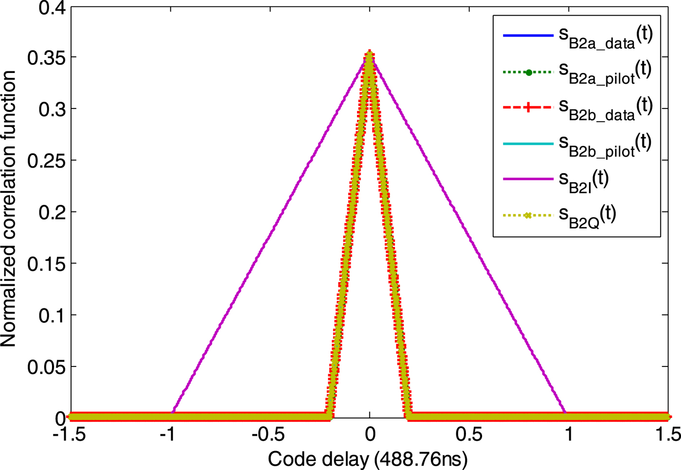
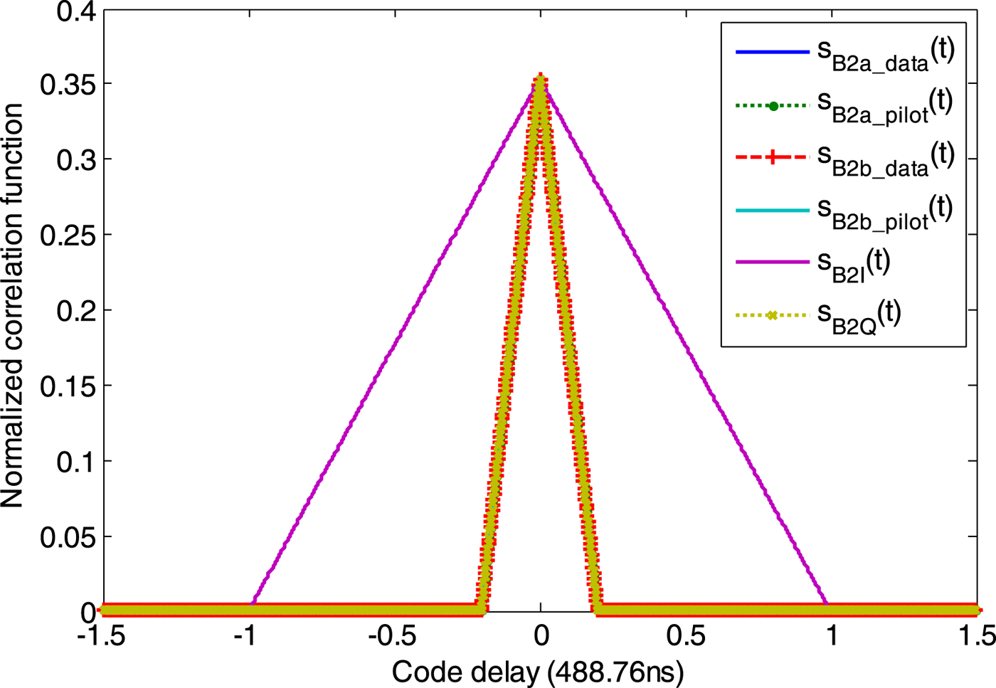
To verify the correctness and effectiveness of the proposed method, the method of Zhang et al. (Reference Zhang, Zhou and Wang2013) is adopted. The correlation functions and Power Spectrum Density (PSD) of the proposed signal with M=32 are obtained by simulation. In simulation, all the signal components use different random PRN codes. These correlation functions shown in Figure 9 are averaged using 1,000 pairs of different random PRN codes. We can see that B2a_data, B2a_pilot, B2b_data, B2b_pilot, B2I and B2Q have almost equal correlation peaks, which are 0·3533, 0·3533, 0·3529, 0·3536, 0·3532 and 0·3532, respectively. The shape of these correlation functions of B2a_data, B2a_pilot, B2b_data, B2b_pilot and B2Q is the auto-correlation function of BPSK(10), and the shape of the correlation function of B2I is the auto-correlation function of BPSK(2).
The simulated correlation functions.
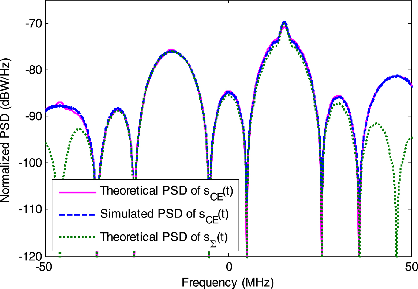
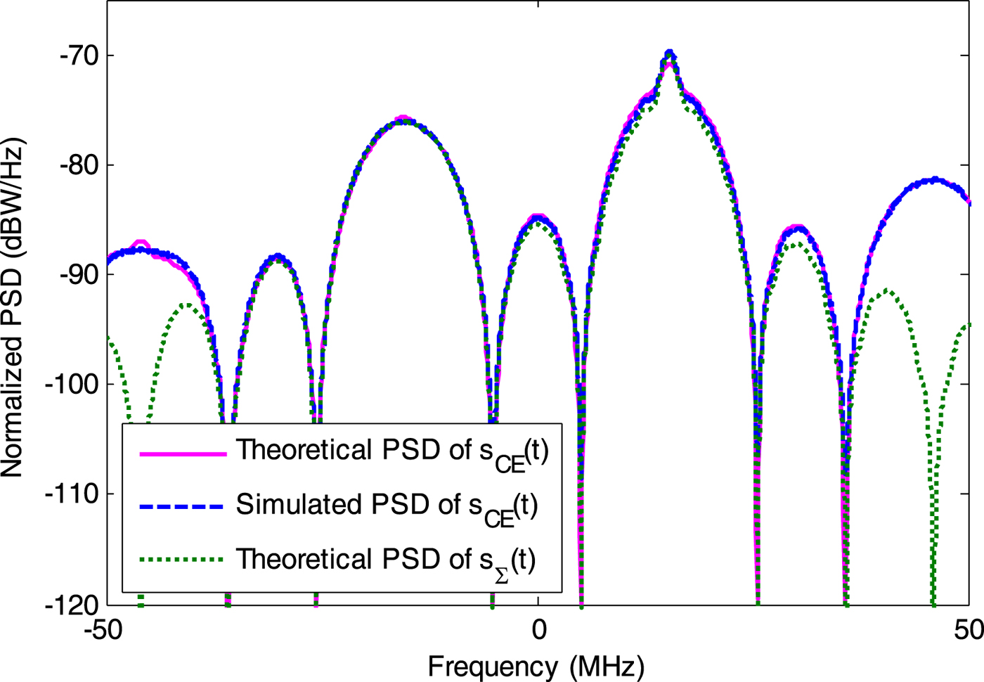
To analyse the PSD of the proposed B2 signal, the theoretical PSD can be calculated following the derivation of Yao et al. (Reference Yao, Zhang and Lu2016). Figure 10 shows the simulated and theoretical PSDs of the proposed B2 signal. For comparison, the theoretical PSD of the linear combination of useful signal components is also provided. It can be seen that the simulated and theoretical PSDs agree well on the whole but there is still a slight deviation between the simulated and theoretical PSDs. Parts of these differences come from numerical errors, such as truncation and rounding errors. The other parts of these differences result from the finite sampling rate and non-ideal PRN codes. The shapes of the main lobes in the simulated PSD are basically the same as those in the theoretical PSD of S Σ(t), which demonstrates that the proposed design method is efficient. It can be noted that the PSD difference between s CE(t) and S Σ(t) results from the inter-modulation terms and high-order harmonic components.
The simulated PSD.
The simulation results above show that the proposed design method can achieve DCEM efficiently and modulate each signal component to the designed frequency.
6. CONCLUSIONS
The DCEM method is currently a popular topic in GNSS signal design research. New DCEM methods, such as generalised AltBOC, ACE-BOC, ES ACE-BOC and BS-ACEBOC have been proposed. Compared with AltBOC, these emerging DCEM methods have a significant improvement in flexibility. However, results show that these existing DCEM methods can reach optimal performance only for some special cases. This paper proposes a unified DCEM design framework for GNSS signals. The existing DCEM methods can be unified in our framework. The proposed design method has no special constraints on the phase relationship and power allocation of signal components. The performance analysis results show that the proposed method can reach higher multiplexing efficiency compared with generalised AltBOC, ACE-BOC and ES ACE-BOC. In addition, the proposed method can satisfy the requirement of backward compatibility in GNSS signal design. As an example, we propose a DCEM scheme for the BDS B2 signal. The theory and simulation results verify the correctness and effectiveness of the proposed method. In summary, the proposed unified DCEM design framework has significant potential.
ACKNOWLEDGEMENT
This work is supported by the National Natural Science Foundation of China (NSFC), Grant 61627817.