1 Introduction
It is known that the no-motion state of a thin film heated from below is subject to two kinds of monotonic Marangoni instability, the Pearson (Pearson Reference Pearson1958) and deformational (Scriven & Sternling Reference Scriven and Sternling1964; Smith Reference Smith1966) ones. Pearson’s mode develops when no surface deformation occurs, i.e. surface tension is high or the gravity is strong. This instability is typically short-wave with the finite critical wavenumber
 $q$
, but in the case of small Biot number,
 $Bi$
, the critical wavenumber is small,
 $q\sim Bi^{1/4}$
. The deformational mode is a long-wave one with zero critical wavenumber, it occurs in very thin layers or under reduced gravity. Recently, Shklyaev, Khenner & Alabuzhev (Reference Shklyaev, Khenner and Alabuzhev2012) showed that coupling of both modes creates an oscillatory mode, which can be critical in the case of a substrate of low heat conductivity.
It is important to be able to control convection from the point of view of both technology and fundamental science. For engineering applications, the long-wavelength mode of instability can be harmful for many processes because of its tendency to rupture the film. For fundamental science, the ability to stabilize the otherwise unstable states promotes deeper understanding of the mechanisms of instabilities.
To stabilize the no-motion state of a thin film heated from below we apply feedback control. Instead of ‘open-loop’ control (vibrations, modulation of parameters, etc), the feedback control is less invasive and almost vanishes when the desired state of the system is achieved. The feedback control has been successfully applied for the suppression of instabilities in large-aspect-ratio systems in the case of the Rayleigh–Bénard convection, both theoretically (Tang & Bau Reference Tang and Bau1994) and in experiments (Howle Reference Howle1997; Tang & Bau Reference Tang and Bau1998); a survey can be found in Shklyaev & Nepomnyashchy (Reference Shklyaev and Nepomnyashchy2017).
We use proportional linear feedback control, the principle of which is that we feed information about the instability back into the dynamics by changing the heat flux through the substrate that can affect the instability. Strategy (I) uses the interfacial deflection from the mean position as the criterion of instability onset (as in Or et al. Reference Or, Kelly, Cortelezzi and Speyer1999). Within strategy (II) the variable that describes the instability is the deviation of the measured temperatures from the desired, conductive values (as in Bau Reference Bau1999).
The present paper is devoted to finding the most effective control strategy among the two mentioned above to delay the onset of instability. We perform two types of calculation. The first is the linear analysis of the long-wave amplitude equations. We derive these nonlinear equations using the lubrication approximation, which is a simplification of the problem, but at the same time a very powerful and frequently used approach (Oron, Davis & Bankoff Reference Oron, Davis and Bankoff1997; Craster & Matar Reference Craster and Matar2009). The second is the linear stability analysis that is carried out within the full Bénard–Marangoni problem for arbitrary wavelengths.
The analysis is carried out under some simplifying assumptions. Following Bau (Reference Bau1999), we assume that the sensors and actuators are continuously distributed. Also, we disregard the heat dynamics transfer inside the solid substrate (recently studied by Batson et al. Reference Batson, Cummings, Shirokoff and Kondic2019) and assume that we can directly modify the heat flux at the boundary between the liquid film and solid substrate at any point.
The paper is organized as follows. We start with the mathematical formulation of the uncontrolled convection in § 2. The control strategies are described in detail in § 3. In § 4 we derive, using the lubrication approximation, a set of amplitude equations which govern the coupled evolution of the layer thickness and the characteristic temperature. There we perform the linear stability analysis within different control strategies. The neutral stability curves for monotonic and oscillatory modes are provided. In § 5 we perform the linear stability analysis within the Marangoni problem for arbitrary wavelengths. The comparison of the results for different control strategies is presented. The paper is finalized with a summary in § 6.
2 Mathematical model of convection
We consider a horizontal liquid layer confined between a deformable free upper surface and a solid bottom wall. The layer is heated from below; the thermal conductivity of the liquid
 $\unicode[STIX]{x1D705}$
is assumed to be large in comparison with that of the substrate, so that the vertical component of the heat flux
 $\unicode[STIX]{x1D705}A$
is fixed. The unperturbed layer thickness
 $H$
is considered sufficiently small, so that the influence of buoyancy is negligible and the free surface deformation is important. The surface tension decreases linearly with the temperature:
 $\unicode[STIX]{x1D6FC}=\unicode[STIX]{x1D6FC}_{0}-\unicode[STIX]{x1D6FC}_{T}T$
, where
 $T$
is the deviation of temperature from a reference one, which is the temperature of the gas above the liquid layer. The heat flux from the free surface is governed by Newton’s law of cooling. The Cartesian reference frame is chosen in such a way that the x- and y-axes are in the substrate plane and the z-axis is normal to the substrate.
The uncontrolled surface-tension-driven convection in this layer is governed by the following system of dimensionless equations and boundary conditions (Nepomnyashchy, Simanovskii & Legros Reference Nepomnyashchy, Simanovskii and Legros2012):
 $$\begin{eqnarray}\frac{1}{Pr}\left(\frac{\unicode[STIX]{x2202}\boldsymbol{v}}{\unicode[STIX]{x2202}t}+\boldsymbol{v}\boldsymbol{\cdot }\unicode[STIX]{x1D735}\boldsymbol{v}\right)=-\unicode[STIX]{x1D735}p+\unicode[STIX]{x1D6FB}^{2}\boldsymbol{v}-Ga\boldsymbol{k},\quad \frac{\unicode[STIX]{x2202}T}{\unicode[STIX]{x2202}t}+\boldsymbol{v}\boldsymbol{\cdot }\unicode[STIX]{x1D735}T=\unicode[STIX]{x1D6FB}^{2}T,\quad \unicode[STIX]{x1D735}\boldsymbol{\cdot }\boldsymbol{v}=0,\end{eqnarray}$$
 $$\begin{eqnarray}z=0:\boldsymbol{v}=0,\quad \frac{\unicode[STIX]{x2202}T}{\unicode[STIX]{x2202}z}=-1,\end{eqnarray}$$
 $$\begin{eqnarray}z=h(x,y,t):\frac{\unicode[STIX]{x2202}h}{\unicode[STIX]{x2202}t}=w-\boldsymbol{u}\boldsymbol{\cdot }\unicode[STIX]{x1D735}h,\quad \unicode[STIX]{x1D749}^{(i)}\boldsymbol{\cdot }\unicode[STIX]{x1D748}\boldsymbol{\cdot }\boldsymbol{n}=-Ma\unicode[STIX]{x1D749}^{(i)}\boldsymbol{\cdot }\unicode[STIX]{x1D735}(T|_{z=h}),\end{eqnarray}$$
 $$\begin{eqnarray}\boldsymbol{n}\boldsymbol{\cdot }\unicode[STIX]{x1D748}\boldsymbol{\cdot }\boldsymbol{n}=p-CaK,\quad \frac{\unicode[STIX]{x2202}T}{\unicode[STIX]{x2202}n}=-BiT,\end{eqnarray}$$
where
 $\boldsymbol{v}=(\boldsymbol{u},w)$
is the velocity field (where
 $\boldsymbol{u}$
is the velocity in the
 $(x,y)$
-plane and
 $w$
is the
 $z$
component),
 $T$
is the temperature,
 $p$
is the pressure in the liquid (measured from the atmospheric pressure),
 $\unicode[STIX]{x1D748}$
is the viscous stress tensor,
 $\boldsymbol{k}$
is the upward unit vector,
 $h$
is the local layer thickness,
 $\boldsymbol{n}$
is the normal unit vector at the free surface,
 $K$
is the curvature of the free surface
 $$\begin{eqnarray}K=-\left(\unicode[STIX]{x1D6FB}^{2}h+\frac{\unicode[STIX]{x2202}^{2}h}{\unicode[STIX]{x2202}x^{2}}\left(\frac{\unicode[STIX]{x2202}h}{\unicode[STIX]{x2202}y}\right)^{2}+\frac{\unicode[STIX]{x2202}^{2}h}{\unicode[STIX]{x2202}y^{2}}\left(\frac{\unicode[STIX]{x2202}h}{\unicode[STIX]{x2202}x}\right)^{2}\right)(1+(\unicode[STIX]{x1D735}h)^{2})^{-3/2},\end{eqnarray}$$
and
 $\unicode[STIX]{x1D749}^{(i)},i=1,2$
are orthonormal tangent vectors to the free surface. We use the following scalings:
 $H$
for the length,
 $H^{2}/\unicode[STIX]{x1D712}$
for the time,
 $\unicode[STIX]{x1D712}/H$
for the velocity,
 $\unicode[STIX]{x1D70C}\unicode[STIX]{x1D708}\unicode[STIX]{x1D712}/H^{2}$
for the pressure,
 $AH$
for the temperature (here
 $\unicode[STIX]{x1D712}$
is the thermal diffusivity,
 $\unicode[STIX]{x1D70C}$
is the density and
 $\unicode[STIX]{x1D708}$
is the kinematic viscosity). The problem is characterized by the following dimensionless parameters:
 $$\begin{eqnarray}Ca=\frac{\unicode[STIX]{x1D6FC}_{0}H}{\unicode[STIX]{x1D70C}\unicode[STIX]{x1D708}\unicode[STIX]{x1D712}},\quad Ma=\frac{\unicode[STIX]{x1D6FC}_{T}AH^{2}}{\unicode[STIX]{x1D70C}\unicode[STIX]{x1D708}\unicode[STIX]{x1D712}},\quad Ga=\frac{g_{0}H^{3}}{\unicode[STIX]{x1D708}\unicode[STIX]{x1D712}},\quad Pr=\frac{\unicode[STIX]{x1D708}}{\unicode[STIX]{x1D712}},\quad Bi=\frac{QH}{\unicode[STIX]{x1D705}},\end{eqnarray}$$
which are the capillary, Marangoni, Galileo, Prandtl and Biot numbers, respectively;
 $Q$
is the heat transfer coefficient.
The conductive state of this system is given by the following expressions:
 $$\begin{eqnarray}\boldsymbol{v}^{(0)}=0,\quad p^{(0)}=Ga(1-z),\quad T^{(0)}=1-z+\frac{1}{Bi},\quad h^{(0)}=1,\end{eqnarray}$$
that correspond to the hydrostatic pressure and linear temperature distribution in a motionless liquid with a planar free surface.
The linear stability of the conductive state provides the critical Marangoni number
 $Ma_{c}$
. Above that value, solution (2.7) becomes unstable. In this paper we investigate control strategies to maintain a stable no-motion state under conditions in which such a state would otherwise be unstable.
3 Control strategies
The physical mechanism of control is based on the suppression of the surface-tension-induced flow. When fluid starts to rise during the convective motion the controllers detect this and direct the actuator to lower the heat flux. In turn the rising fluid will carry less excess temperature than without control. As a result the surface-tension-induced currents will be weaker, allowing ample time for heat dissipation to equalize the surface temperature and restore the no-motion state.
In this paper we consider two types of detector. The first one is capable of detecting the level of the free surface (control strategy (I)). The second one measures the departure of the fluid temperature from its conductive value (control strategy (II)). Both strategies can be carried out optically and non-intrusively, also they are relatively easy to implement (Howle Reference Howle1997; Benz et al. Reference Benz, Hintz, Riley and Neitzel1998).
The actuator modifies the heat flux through the substrate according to the rules
 $$\begin{eqnarray}\displaystyle \text{(I)}:\quad \left.\frac{\unicode[STIX]{x2202}T}{\unicode[STIX]{x2202}z}\right|_{z=0}=-1-K_{s}(h-1),\quad \text{or} & & \displaystyle\end{eqnarray}$$
 $$\begin{eqnarray}\displaystyle \text{(IIa)}:\quad \left.\frac{\unicode[STIX]{x2202}T}{\unicode[STIX]{x2202}z}\right|_{z=0}=-1-K_{T}(T-T^{(0)})|_{z=1/2},\quad \text{or} & & \displaystyle\end{eqnarray}$$
 $$\begin{eqnarray}\displaystyle \text{(IIb)}:\quad \left.\frac{\unicode[STIX]{x2202}T}{\unicode[STIX]{x2202}z}\right|_{z=0}=-1-K_{Ts}(T|_{z=h}-T^{(0)}|_{z=1}), & & \displaystyle\end{eqnarray}$$
where
 $K_{s}$
,
 $K_{T}$
and
 $K_{Ts}$
are non-dimensional scalar control gains. It should be noted that
 $K_{s}>0$
and
 $K_{T,Ts}<0$
correspond to a reduced heat flux at the lower wall for a positive temperature perturbation and vice versa.
Note that strategy (II) is applied in two ways. Recall that in the case of a non-deformable free surface Tang & Bau (Reference Tang and Bau1994) applied the feedback control law as
 $$\begin{eqnarray}\left.\frac{\unicode[STIX]{x2202}T}{\unicode[STIX]{x2202}z}\right|_{z=0}=-1-K_{T}(T-T^{(0)})|_{z=1},\end{eqnarray}$$
i.e. the deviation of the interior temperature from its conductive value is measured by detectors that are placed at the
 $z=1$
. This control strategy should be modified in the case of deformable surface. Indeed, let us assume that convective motion results in such a deflection of free surface that it becomes below its mean value at a particular point. In this situation the measurements of the detectors attached to the position
 $z=1$
are no longer adequate. That difficulty can be resolved by measuring the temperature in the middle of the layer (Tang & Bau Reference Tang and Bau1998), which corresponds to control strategy (IIa).
Alternatively, the detectors can be designed in such a way that they measure temperature at the free deformable surface, then the control strategy (IIb) can be applied. In this paper we use both versions of strategy (II).
It is worth noting that (2.7) is a solution for each of the control techniques. Hence, the control does not disturb the conductive state. In § 4 we study the stability of this solution with respect to long-wave perturbations and the evolution of the large-scale perturbations to the conductive state. In § 5 we extend our linear analysis to finite wavelengths.
4 Amplitude equations
4.1 Lubrication approximation
To study the evolution of large-scale flows, we rescale the coordinates, the time and the velocity according to the relations (Shklyaev et al. Reference Shklyaev, Khenner and Alabuzhev2012)
 $$\begin{eqnarray}X=\unicode[STIX]{x1D700}x,\quad Y=\unicode[STIX]{x1D700}y,\quad Z=z,\quad \unicode[STIX]{x1D70F}=\unicode[STIX]{x1D700}^{2}t,\quad \boldsymbol{U}=\unicode[STIX]{x1D700}^{-1}\boldsymbol{u},\quad W=\unicode[STIX]{x1D700}^{-2}w,\end{eqnarray}$$
where
 $\unicode[STIX]{x1D700}\ll 1$
can be thought of as the ratio of
 $H$
to a typical horizontal length scale.
Then we expand all the fields in power series with respect to
 $\unicode[STIX]{x1D700}^{2}$
 $$\begin{eqnarray}\left.\begin{array}{@{}c@{}}\boldsymbol{U}=\boldsymbol{U}_{0}+\unicode[STIX]{x1D700}^{2}\boldsymbol{U}_{1}+\cdots \,,\quad W=W_{0}+\unicode[STIX]{x1D700}^{2}W_{1}+\cdots \,,\\ p=p_{0}+\unicode[STIX]{x1D700}^{2}p_{1}+\cdots \,,\quad T=-z+{\displaystyle \frac{1}{Bi}}+T_{0}+\unicode[STIX]{x1D700}^{2}T_{1}+\cdots \end{array}\right\}.\end{eqnarray}$$
We do not write an expansion for
 $h$
for the sake of brevity. The perturbations of the local layer thickness, temperature and pressure are not required to be small; however, the perturbation gradients must be small. Also, we do not remove the equilibrium fields from
 $T$
and
 $p$
; it is clear that the base conductive state corresponds to
 $T_{0}=1$
,
 $p_{0}=p^{(0)}$
.
We apply the same scaling as in Shklyaev et al. (Reference Shklyaev, Khenner and Alabuzhev2012) as we focus on the novel oscillatory mode. This mode emerges at large values of Ca, small Biot number and finite Galileo number
 $$\begin{eqnarray}Ca=\unicode[STIX]{x1D700}^{-2}C,\quad Bi=\unicode[STIX]{x1D700}^{2}\unicode[STIX]{x1D6FD},\quad Ga=O(1).\end{eqnarray}$$
We also assume the following scaling for the feedback control gain
 $$\begin{eqnarray}K_{T,s}=\unicode[STIX]{x1D700}^{2}\unicode[STIX]{x1D718}_{T,s}.\end{eqnarray}$$
Substituting equations (4.1)–(4.4) into (2.1)–(2.4) and using one of the control laws (3.1), (3.2) or (3.3), we obtain at the zeroth order the boundary-value problem
 $$\begin{eqnarray}\frac{\unicode[STIX]{x2202}W_{0}}{\unicode[STIX]{x2202}Z}=-\unicode[STIX]{x1D735}_{2}\boldsymbol{\cdot }\boldsymbol{U}_{0},\quad \frac{\unicode[STIX]{x2202}p_{0}}{\unicode[STIX]{x2202}Z}=-Ga,\quad \frac{\unicode[STIX]{x2202}^{2}\boldsymbol{U}_{0}}{\unicode[STIX]{x2202}Z^{2}}=\unicode[STIX]{x1D735}_{2}p_{0},\quad \frac{\unicode[STIX]{x2202}^{2}T_{0}}{\unicode[STIX]{x2202}Z^{2}}=0,\end{eqnarray}$$
 $$\begin{eqnarray}z=0:\boldsymbol{U}_{0}=W_{0}=\frac{\unicode[STIX]{x2202}T_{0}}{\unicode[STIX]{x2202}Z}=0,\end{eqnarray}$$
 $$\begin{eqnarray}z=h:\frac{\unicode[STIX]{x2202}h}{\unicode[STIX]{x2202}\unicode[STIX]{x1D70F}}=-\boldsymbol{U}_{0}\unicode[STIX]{x1D735}h+W_{0},\quad p_{0}=-C\unicode[STIX]{x1D735}_{2}^{2}h,\quad \frac{\unicode[STIX]{x2202}\boldsymbol{U}_{0}}{\unicode[STIX]{x2202}Z}=-Ma\unicode[STIX]{x1D735}_{2}(T_{0}-h),\quad \frac{\unicode[STIX]{x2202}T_{0}}{\unicode[STIX]{x2202}z}=0,\end{eqnarray}$$
which is identical to the uncontrolled one as expected. Hereinafter
 $\unicode[STIX]{x1D735}_{2}=(\unicode[STIX]{x2202}/\unicode[STIX]{x2202}X,\unicode[STIX]{x2202}/\unicode[STIX]{x2202}Y,0)$
.
The evolution of the layer thickness is governed by the well-known condition
 $\unicode[STIX]{x2202}h/\unicode[STIX]{x2202}\unicode[STIX]{x1D70F}=-\unicode[STIX]{x1D735}_{2}\boldsymbol{\cdot }\int _{0}^{h}\boldsymbol{U}_{0}\,\text{d}Z$
. As the control terms do not appear at the zeroth order, the first amplitude equation remains the same as in Shklyaev et al. (Reference Shklyaev, Khenner and Alabuzhev2012).
 $$\begin{eqnarray}\frac{\unicode[STIX]{x2202}h}{\unicode[STIX]{x2202}\unicode[STIX]{x1D70F}}=\unicode[STIX]{x1D735}_{2}\boldsymbol{\cdot }\left(\frac{h^{3}}{3}\unicode[STIX]{x1D735}_{2}P+Ma\frac{h^{2}}{2}\unicode[STIX]{x1D735}_{2}\,f\right)\equiv \unicode[STIX]{x1D735}_{2}\boldsymbol{\cdot }\boldsymbol{j},\end{eqnarray}$$
where
 $P=Gah-C\unicode[STIX]{x1D735}_{2}^{2}h$
,
 $f=\unicode[STIX]{x0398}-h$
,
 $T_{0}=\unicode[STIX]{x0398}(X,Y,\unicode[STIX]{x1D70F})$
. The vector
 $-\boldsymbol{j}$
has the meaning of the longitudinal flux of a liquid averaged across the layer.
The second amplitude equation is obtained from the first order of the expansion where we need only the equations that describe heat transfer in the liquid. The partial differential equation that describes the heat transfer through the layer remains the same as in the uncontrolled case
 $$\begin{eqnarray}\frac{\unicode[STIX]{x2202}^{2}T_{1}}{\unicode[STIX]{x2202}Z^{2}}=\frac{\unicode[STIX]{x2202}\unicode[STIX]{x0398}}{\unicode[STIX]{x2202}\unicode[STIX]{x1D70F}}-\unicode[STIX]{x1D6FB}_{2}^{2}\unicode[STIX]{x0398}+\boldsymbol{U}_{0}\boldsymbol{\cdot }\unicode[STIX]{x1D735}_{2}\unicode[STIX]{x0398}-W_{0},\end{eqnarray}$$
as well as the boundary condition at the free surface
 $$\begin{eqnarray}\left.\frac{\unicode[STIX]{x2202}T_{1}}{\unicode[STIX]{x2202}Z}\right|_{Z=h}=\unicode[STIX]{x1D735}_{2}\unicode[STIX]{x0398}\boldsymbol{\cdot }\unicode[STIX]{x1D735}_{2}h-\frac{1}{2}(\unicode[STIX]{x1D735}_{2}h)^{2}-\unicode[STIX]{x1D6FD}f.\end{eqnarray}$$
However, the heat flux condition at the substrate depends on the feedback control law. The solvability condition of the latter problem provides the second amplitude equation. Below we derive this amplitude equation for different control strategies and compare it with the uncontrolled case.
4.2 Uncontrolled convection
The amplitude equations for uncontrolled convection were derived and investigated by Shklyaev et al. (Reference Shklyaev, Khenner and Alabuzhev2012). For reader convenience, we briefly present the results of the cited paper.
The solvability condition of (4.9) with the boundary conditions (4.10) and
 $\unicode[STIX]{x2202}T_{1}/\unicode[STIX]{x2202}Z|_{Z=0}=0$
results in
 $$\begin{eqnarray}h\frac{\unicode[STIX]{x2202}\unicode[STIX]{x0398}}{\unicode[STIX]{x2202}\unicode[STIX]{x1D70F}}=\unicode[STIX]{x1D735}_{2}\boldsymbol{\cdot }(h\unicode[STIX]{x1D735}_{2}\unicode[STIX]{x0398})-\frac{1}{2}(\unicode[STIX]{x1D735}_{2}h)^{2}-\unicode[STIX]{x1D6FD}f+\boldsymbol{j}\boldsymbol{\cdot }\unicode[STIX]{x1D735}_{2}\,f+\unicode[STIX]{x1D735}\boldsymbol{\cdot }\left(\frac{h^{4}}{8}\unicode[STIX]{x1D735}_{2}P+\frac{h^{3}}{6}Ma\unicode[STIX]{x1D735}_{2}\,f\right).\end{eqnarray}$$
Equations (4.8) and (4.11) form a closed set of amplitude equations, which governs the nonlinear dynamics of long-wave perturbations. These equations include the following effects: on the right-hand side of (4.8), damping of the surface deflection due to gravity and surface tension, and the influence of the thermocapillary flow on the layer thickness; on the right-hand side of (4.11), heat conductivity in the longitudinal directions (the first term), heat losses from the free surface [the second and third terms, where the second term describes the effect originating from the increase of the surface area (at constant volume)], and advective heat transfer by the flow (the fourth and fifth terms).
The base state, corresponding to a motionless fluid and gas with a constant heat flux maintained through the layers, is given by
 $h=1$
and
 $\unicode[STIX]{x0398}=1$
.
Linear stability analysis of amplitude equations (4.8), (4.11) for normal perturbations proportional to
 $\exp (\unicode[STIX]{x1D706}\unicode[STIX]{x1D70F}+\text{i}(k_{X}X+k_{Y}Y))$
provides a system of two algebraic equations that gives the relation between the amplitudes of the perturbations, see appendix A. The solvability condition of this system results in the neutral stability curves for the monotonic (
 $Ma^{m}$
) and the oscillatory (
 $Ma^{o}$
) modes
 $$\begin{eqnarray}Ma^{m}=\frac{48(\unicode[STIX]{x1D6FD}+k^{2})(Ga+Ck^{2})}{k^{2}(72+Ga+Ck^{2})},\quad Ma^{o}=3+Ga+Ck^{2}+\frac{3\unicode[STIX]{x1D6FD}}{k^{2}},\end{eqnarray}$$
where
 $k^{2}=k_{X}^{2}+k_{Y}^{2}$
. This wavenumber
 $k$
is connected with the unscaled wavenumber
 $q$
as
 $$\begin{eqnarray}q=\unicode[STIX]{x1D700}k,\end{eqnarray}$$
which implies the scaling
 $q\sim Bi^{1/2}$
in accordance with (4.3). In fact, this means that we deal with smaller values of the wavenumber than those implied by the usual scaling
 $q\sim Bi^{1/4}$
.
Note that the monotonic neutral curve has a minimum at finite values of
 $k$
only if
 $\unicode[STIX]{x1D6FD}C<72$
, otherwise the short-wave mode is critical: the minimum
 $Ma_{\ast }^{m}=48$
is achieved in the limit
 $k\rightarrow \infty$
. Recall that
 $Ma=48$
represents the minimum of the Pearson monotonic mode for a non-deformable surface for
 $Bi=0$
. Thus, the ‘short-wave mode’ corresponds in fact to small wavenumbers
 $Bi^{1/2}\ll q\ll Bi^{1/4}\ll 1$
.
The imaginary part of the growth rate (frequency) for neutral oscillatory perturbations is
 $$\begin{eqnarray}\unicode[STIX]{x1D714}=\frac{k^{2}}{12}\sqrt{(72+Ga+Ck^{2})(Ma^{m}-Ma^{o})}.\end{eqnarray}$$
It is clear that the oscillatory mode is present only if
 $Ma^{m}>Ma^{o}$
.
Below we investigate how the feedback control affects the onset of this long-wave instability.
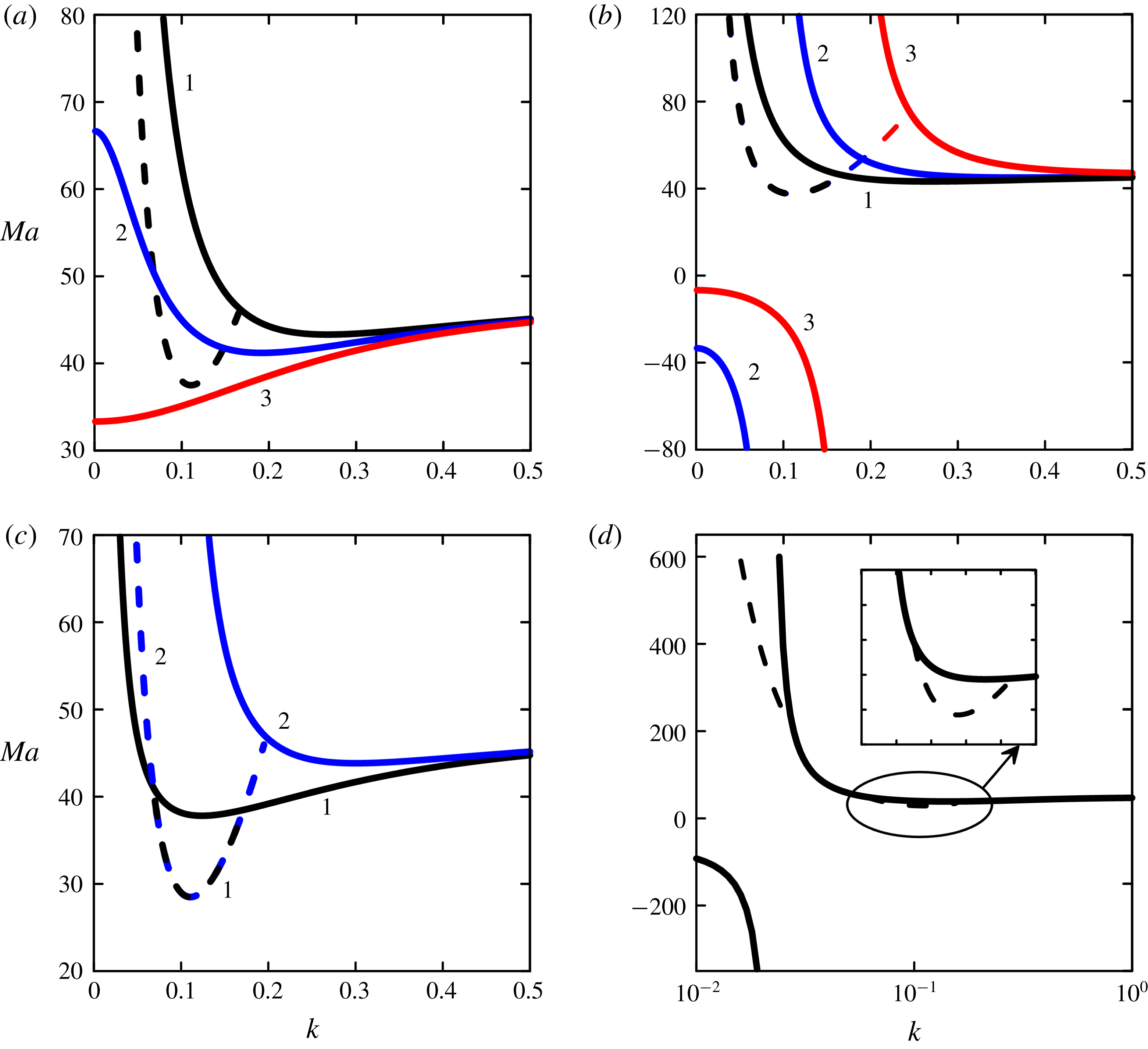
Neutral stability curves for the monotonic (solid lines) and the oscillatory (dashed lines) long-wave modes for control strategy (I).
 $Pr=1$
,
 $C=1000$
,
 $\unicode[STIX]{x1D6FD}=0.05$
. Panels (a,b) correspond to
 $Ga=10$
. Lines 1, 2 and 3 correspond to (a)
 $\unicode[STIX]{x1D718}_{s}=0$
,
 $\unicode[STIX]{x1D718}_{s}=-0.005$
and
 $\unicode[STIX]{x1D718}_{s}=-0.01$
; (b)
 $\unicode[STIX]{x1D718}_{s}=0$
,
 $\unicode[STIX]{x1D718}_{s}=0.01$
and
 $\unicode[STIX]{x1D718}_{s}=0.05$
, respectively. Panels (c,d) correspond to
 $Ga=1$
. Lines 1 and 2 correspond to
 $\unicode[STIX]{x1D718}_{s}=0$
and
 $\unicode[STIX]{x1D718}_{s}=0.01$
, respectively (c). Panel (d) depicts
 $\unicode[STIX]{x1D718}_{s}=0.0005$
.

4.3 Control strategy (I)
As we focus on the instability which is significantly determined by the free surface deformation, it looks reasonable to apply the control by the deflection of the free surface from planarity.
Control law (3.1) with the scaling (4.4) in the first order of expansion becomes
 $$\begin{eqnarray}\left.\frac{\unicode[STIX]{x2202}T_{1}}{\unicode[STIX]{x2202}Z}\right|_{Z=0}=-\unicode[STIX]{x1D718}_{s}(h-1).\end{eqnarray}$$
The second amplitude equation for this control strategy is
 $$\begin{eqnarray}h\frac{\unicode[STIX]{x2202}\unicode[STIX]{x0398}}{\unicode[STIX]{x2202}\unicode[STIX]{x1D70F}}=\unicode[STIX]{x1D735}_{2}\boldsymbol{\cdot }(h\unicode[STIX]{x1D735}_{2}\unicode[STIX]{x0398})-\frac{1}{2}(\unicode[STIX]{x1D735}_{2}h)^{2}-\unicode[STIX]{x1D6FD}f+\unicode[STIX]{x1D718}_{s}(h-1)+\boldsymbol{j}\boldsymbol{\cdot }\unicode[STIX]{x1D735}_{2}f+\unicode[STIX]{x1D735}_{2}\boldsymbol{\cdot }\!\left(\frac{h^{4}}{8}\unicode[STIX]{x1D735}_{2}P+\frac{h^{3}}{6}Ma\unicode[STIX]{x1D735}_{2}\,f\right)\!.\end{eqnarray}$$
In comparison with the uncontrolled equation (4.11) the additional linear term concerned with the free surface deflection appears here. The linear stability analysis of (4.11) and (4.16) with respect to the normal perturbations gives the neutral curves and the dispersion relation
 $$\begin{eqnarray}Ma^{m}=\frac{48(Ga+Ck^{2})(k^{2}+\unicode[STIX]{x1D6FD})}{k^{2}(72+Ga+Ck^{2})-72\unicode[STIX]{x1D718}_{s}},\quad Ma^{o}=3+Ga+Ck^{2}+\frac{3\unicode[STIX]{x1D6FD}}{k^{2}},\end{eqnarray}$$
 $$\begin{eqnarray}\unicode[STIX]{x1D714}=\frac{k^{2}}{12}\sqrt{\left(72+Ga+Ck^{2}-72\frac{\unicode[STIX]{x1D718}_{s}}{k^{2}}\right)(Ma^{m}-Ma^{o})}.\end{eqnarray}$$
Surprisingly, this control strategy does not affect the oscillatory neutral curve (only the frequency of perturbations is changed). On the contrary, the neutral curves of the monotonic mode change significantly compared with the uncontrolled situation. For example, now the neutral curve has a finite limit of
 $Ma^{m}$
at
 $k\rightarrow 0$
 $$\begin{eqnarray}Ma_{0}^{m}=-\frac{2Ga}{3\unicode[STIX]{x1D6FD}\unicode[STIX]{x1D718}_{s}}.\end{eqnarray}$$
The influence of the linear feedback control (I) on the monotonic mode of the Marangoni instability is presented in figure 1. In the case
 $\unicode[STIX]{x1D718}_{s}<0$
the neutral curves have a finite Ma at
 $k=0$
; the minimum of the neutral curve goes down with increasing control, see solid lines in figure 1(a). At
 $\unicode[STIX]{x1D718}_{s}=-Ga\unicode[STIX]{x1D6FD}(72+Ga)/72(C\unicode[STIX]{x1D6FD}+Ga)$
the critical perturbations become monotonic and long-wave, the minimum of the neutral curve is defined by (4.19). Thus, in that case the system is destabilized with respect to the monotonic mode. In the case
 $\unicode[STIX]{x1D718}_{s}>0$
the increase in the control gain results in the delay of the onset of the monotonic mode, see figure 1(b). Note, that for positive
 $\unicode[STIX]{x1D718}_{s}$
the additional monotonic branch emerges at values
 $Ma<0$
. As this branch corresponds to the opposite sign of the thermocapillary effect, it does not become critical by heating from below. The right branch of the monotonic neutral curve is shifted to the short-wave region with increase of the control gain. This results in enhancement of the region of oscillatory instability. Note, that in the interval of wavenumbers where
 $Ma^{m}<0$
, we have
 $Ma^{o}>0>Ma^{m}$
. This is possible because the first factor under the root in (4.18) becomes negative in this region.
It is noteworthy that in some cases the neutral curve for the oscillatory mode has two points of connection to the monotonic neutral curve, see figure 1(c). As mentioned above, the monotonic neutral curve is shifted to the right with the increase of positive control gain, thus the left connection point of the oscillatory neutral curve goes to infinity. However, at very small positive control gain, the oscillatory neutral curve consists of two separate parts, see figure 1(d). With further increase of the control gain, the monotonic neutral curve moves rightward and these two parts of the oscillatory neutral curve merge into one.
Thus, the control strategy (I) with scaling (4.4) is not efficient for stabilization of the system, if there exists an oscillatory instability.
4.4 Control strategy (IIa)
Let us apply now the control strategy where the instability is detected by the departure of the interior fluid temperature from the conductive state.
Substituting the scaling (4.4) into control law (3.2) one obtains at the first order of expansion
 $$\begin{eqnarray}\left.\frac{\unicode[STIX]{x2202}T_{1}}{\unicode[STIX]{x2202}Z}\right|_{Z=0}=-\unicode[STIX]{x1D718}_{T}(\unicode[STIX]{x0398}-1).\end{eqnarray}$$
The solvability condition of (4.9) with boundary conditions (4.10), (4.20) provides us with the following second amplitude equation
 $$\begin{eqnarray}\displaystyle h\frac{\unicode[STIX]{x2202}\unicode[STIX]{x0398}}{\unicode[STIX]{x2202}\unicode[STIX]{x1D70F}} & = & \displaystyle \unicode[STIX]{x1D735}_{2}\boldsymbol{\cdot }(h\unicode[STIX]{x1D735}\unicode[STIX]{x0398})-\frac{1}{2}(\unicode[STIX]{x1D735}_{2}h)^{2}-\unicode[STIX]{x1D6FD}f+\unicode[STIX]{x1D718}_{T}(\unicode[STIX]{x0398}-1)\nonumber\\ \displaystyle & & \displaystyle +\;\boldsymbol{j}\boldsymbol{\cdot }\unicode[STIX]{x1D735}_{2}\,f+\unicode[STIX]{x1D735}_{2}\boldsymbol{\cdot }\left(\frac{h^{4}}{8}\unicode[STIX]{x1D735}_{2}P+\frac{h^{3}}{6}Ma\unicode[STIX]{x1D735}_{2}\,f\right).\end{eqnarray}$$
An additional linear term, that corresponds to the increased (or reduced) average temperature, appears in this amplitude equation in comparison with the uncontrolled equation (4.11). The linear stability analysis of (4.11) and (4.21) with respect to the normal perturbations gives the neutral curves and the dispersion relation
 $$\begin{eqnarray}Ma^{m}=\frac{48(Ga+Ck^{2})(k^{2}+\unicode[STIX]{x1D6FD}-\unicode[STIX]{x1D718}_{T})}{k^{2}(72+Ga+Ck^{2})-72\unicode[STIX]{x1D718}_{T}},\quad Ma^{o}=3+Ga+Ck^{2}+\frac{3(\unicode[STIX]{x1D6FD}-\unicode[STIX]{x1D718}_{T})}{k^{2}},\end{eqnarray}$$
 $$\begin{eqnarray}\unicode[STIX]{x1D714}=\frac{k^{2}}{12}\sqrt{\left(72+Ga+Ck^{2}-72\frac{\unicode[STIX]{x1D718}_{T}}{k^{2}}\right)(Ma^{m}-Ma^{o})}.\end{eqnarray}$$
Note, that instead of the uncontrolled case, the neutral curve of the monotonic instability now has a finite limit
 $Ma^{m}(k\rightarrow 0)$
 $$\begin{eqnarray}Ma_{0}^{m}=\frac{2}{3}\frac{Ga(\unicode[STIX]{x1D718}_{T}-\unicode[STIX]{x1D6FD})}{\unicode[STIX]{x1D718}_{T}}.\end{eqnarray}$$
The change of the neutral stability curve for the oscillatory mode can be described as a variation of the Biot number: parameter
 $\unicode[STIX]{x1D6FD}$
is replaced with
 $\tilde{\unicode[STIX]{x1D6FD}}=\unicode[STIX]{x1D6FD}-\unicode[STIX]{x1D718}_{T}$
. Thus, one needs to use the feedback control with negative control gain,
 $\unicode[STIX]{x1D718}_{T}<0$
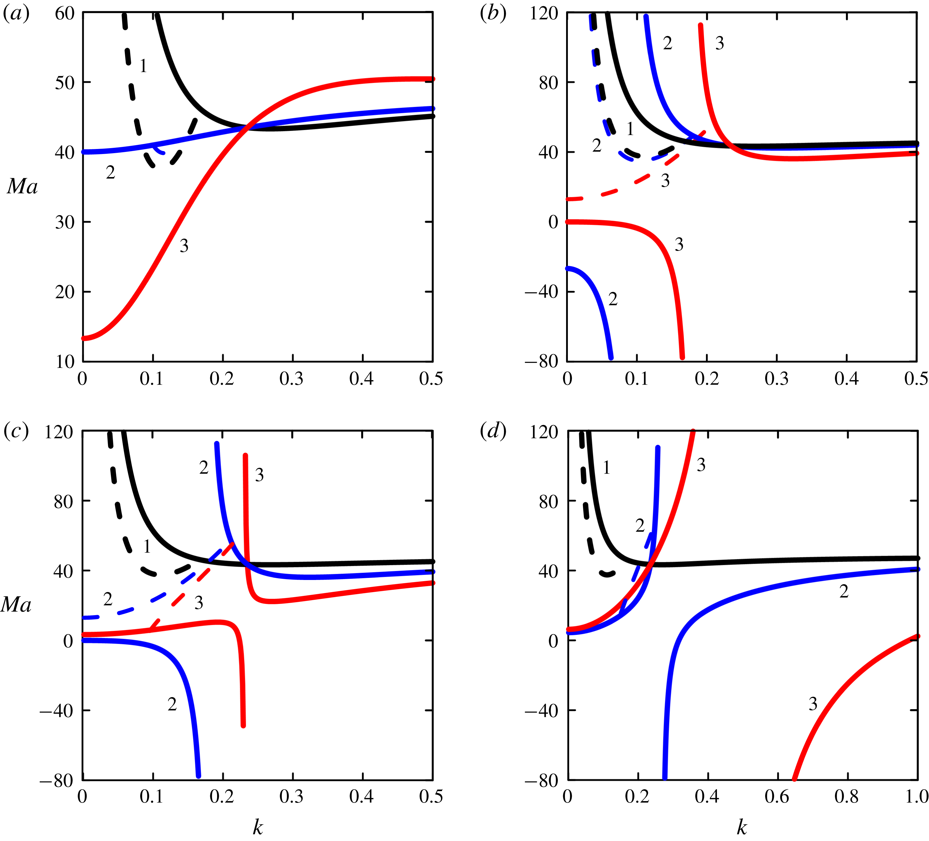
, to suppress the oscillatory mode. However, for the monotonic mode negative control gain results in destabilization of the conductive state, see figure 2(a). Therefore, the given control strategy does not seem appropriate to suppress the instability under consideration.
In figure 2 the influence of the feedback control on the neutral curves of the monotonic (solid lines) and oscillatory (dashed lines) instability is presented. In the case of negative
 $\unicode[STIX]{x1D718}_{T}$
the critical perturbations become monotonic and long-wave with the value of
 $Ma_{c}^{m}$
defined by (4.24). In the case of positive
 $\unicode[STIX]{x1D718}_{T}$
the neutral curves demonstrate a rather interesting variation of their form with the growth of the control gain. While
 $\unicode[STIX]{x1D718}_{T}<\unicode[STIX]{x1D6FD}$
the feedback control slightly destabilizes both the oscillatory and the monotonic modes; wherein the neutral curve for monotonic mode has an additional long-wave branch at
 $Ma<0$
, see figure 2(b).
Neutral stability curves for the monotonic (solid lines) and the oscillatory (dashed lines) long-wave modes for control strategy (IIa).
 $Pr=1$
,
 $Ga=10$
,
 $C=1000$
,
 $\unicode[STIX]{x1D6FD}=0.05$
.
 $\unicode[STIX]{x1D718}_{T}=0$
. Lines 1, 2 and 3 correspond to (a)
 $\unicode[STIX]{x1D718}_{s}=0$
,
 $\unicode[STIX]{x1D718}_{s}=-0.01$
and
 $\unicode[STIX]{x1D718}_{s}=-0.05$
; (b)
 $\unicode[STIX]{x1D718}_{s}=0$
,
 $\unicode[STIX]{x1D718}_{s}=0.01$
and
 $\unicode[STIX]{x1D718}_{s}=0.05$
; (c)
 $\unicode[STIX]{x1D718}_{s}=0$
,
 $\unicode[STIX]{x1D718}_{s}=0.05$
and
 $\unicode[STIX]{x1D718}_{s}=0.1$
; (d)
 $\unicode[STIX]{x1D718}_{s}=0$
,
 $\unicode[STIX]{x1D718}_{s}=0.15$
and
 $\unicode[STIX]{x1D718}_{s}=1$
, respectively.

At
 $\unicode[STIX]{x1D718}_{T}=\unicode[STIX]{x1D6FD}$
the neutral curve for the oscillatory mode becomes a quadratic parabola that starts from
 $Ma_{c}^{o}=3+Ga$
at
 $k=0$
. However, oscillatory mode is not critical as the long-wave branch of the monotonic neutral curve arrives at
 $Ma=0$
. When
 $\unicode[STIX]{x1D718}_{T}>\unicode[STIX]{x1D6FD}$
the neutral curve for the monotonic mode consists of two branches in the area of positive
 $Ma$
, see figure 2(c). The extrema of the right and the left branches (hydrodynamic instability mode and thermal instability mode, respectively) approach each other with the increase of the control gain, whereas the neutral curve for the oscillatory mode becomes the line that connects two monotonic branches.
With further increase in the value of
 $\unicode[STIX]{x1D718}_{T}$
two branches of the monotonic neutral curve reconnect as
 $$\begin{eqnarray}\unicode[STIX]{x1D718}_{T}^{\ast }=\unicode[STIX]{x1D6FD}+\frac{Ga}{2C}\left(\sqrt{\frac{288\unicode[STIX]{x1D6FD}C}{Ga^{2}}+1}-1\right).\end{eqnarray}$$
At
 $\unicode[STIX]{x1D718}_{T}>\unicode[STIX]{x1D718}_{T}^{\ast }$
the left branch of the monotonic neutral curve has the minimum
 $Ma_{0}^{m}$
at
 $k=0$
(see (4.24)), the right branch has the maximum
 $Ma^{m}=48$
in the limit
 $k\rightarrow \infty$
, see figure 2(d). The oscillatory neutral curve is located above the long-wave branch of the monotonic neutral curve. As seen from figure 2(d), the oscillatory mode disappears, and the branches of the monotonic mode move away from each other with the growth of the control gain.
It is noteworthy that within the given control technique special monotonic perturbations exist, which are characterized by the following wavenumber
 $$\begin{eqnarray}k_{\ast }^{2}=\frac{Ga}{2C}\left(\sqrt{\frac{288\unicode[STIX]{x1D6FD}C}{Ga^{2}}+1}-1\right).\end{eqnarray}$$
All monotonic neutral curves intersect at this point, as is seen from figure 2. The perturbations with this particular wavenumber are distinguished by the fact that the temperature perturbation
 $\unicode[STIX]{x0398}$
is absent at any value of control gain. However, such perturbations do not become critical. It is obvious now that the given control technique is not appropriate to suppress the instability under consideration.
4.5 Control strategy (IIb)
Within the considered instability the deformation of the free surface can significantly change the average temperature. Therefore, detecting the departure of the free surface temperature from the conductive state is probably a more appropriate control strategy.
Substituting the scaling (4.4) into control law (3.1) we obtain at the first order of expansion
 $$\begin{eqnarray}\left.\frac{\unicode[STIX]{x2202}T_{1}}{\unicode[STIX]{x2202}Z}\right|_{Z=0}=-\unicode[STIX]{x1D718}_{Ts}(\unicode[STIX]{x0398}-h).\end{eqnarray}$$
The second amplitude equation takes the following form
 $$\begin{eqnarray}h\frac{\unicode[STIX]{x2202}\unicode[STIX]{x0398}}{\unicode[STIX]{x2202}\unicode[STIX]{x1D70F}}=\unicode[STIX]{x1D735}_{2}\boldsymbol{\cdot }(h\unicode[STIX]{x1D735}_{2}\unicode[STIX]{x0398})-\frac{1}{2}(\unicode[STIX]{x1D735}_{2}h)^{2}-(\unicode[STIX]{x1D6FD}-\unicode[STIX]{x1D718}_{Ts})f+\boldsymbol{j}\boldsymbol{\cdot }\unicode[STIX]{x1D735}_{2}\,f+\unicode[STIX]{x1D735}_{2}\boldsymbol{\cdot }\!\left(\frac{h^{4}}{8}\unicode[STIX]{x1D735}_{2}P+\frac{h^{3}}{6}Ma\unicode[STIX]{x1D735}_{2}\,f\right)\!.\end{eqnarray}$$
This equation differs from (4.11) only in the linear term that corresponds to the heat flux through the free surface. Thus, within the given control strategy the instability is suppressed by the mean of the variation of the heat losses from the free surface. Consequently, the feedback control with
 $\unicode[STIX]{x1D718}_{Ts}<0$
suppresses both the monotonic and the oscillatory modes of instability. This is confirmed by the neutral stability curves for the monotonic and oscillatory modes
 $$\begin{eqnarray}Ma^{m}=\frac{48(\unicode[STIX]{x1D6FD}-\unicode[STIX]{x1D718}_{Ts}+k^{2})(Ga+Ck^{2})}{k^{2}(72+Ga+Ck^{2})},\quad Ma^{o}=3+Ga+Ck^{2}+\frac{3(\unicode[STIX]{x1D6FD}-\unicode[STIX]{x1D718}_{Ts})}{k^{2}}.\end{eqnarray}$$
The frequency of the oscillatory perturbations is defined by (4.14).
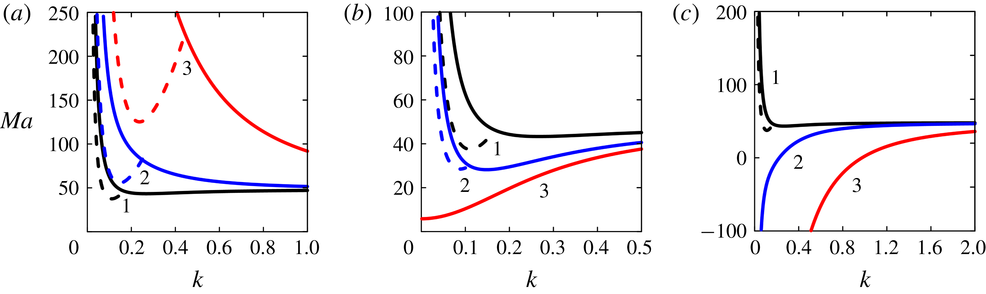
In figure 3 the variations of the neutral curves for the oscillatory (dashed lines) and the monotonic (solid lines) modes with the feedback control gain
 $\unicode[STIX]{x1D718}_{Ts}$
are presented. As expected, strong stabilization of the oscillatory and monotonic modes is observed at any negative value of
 $\unicode[STIX]{x1D718}_{Ts}$
, see figure 3(a). However, at large
 $|\unicode[STIX]{x1D718}_{Ts}|$
our scaling
 $q\sim \sqrt{Bi}$
is no longer adequate, as the minimum of the monotonic neutral curve achieves the short-wave Pearson limit
 $Ma_{c}^{m}=48$
at
 $k\rightarrow \infty$
.
At positive values of the control gain the neutral stability curves go down from the uncontrolled curve. With the increase of
 $\unicode[STIX]{x1D718}_{Ts}$
the oscillatory mode vanishes and the minimum of the monotonic neutral curve moves to the long-wave area, where it achieves the long-wave limit
 $Ma_{c}^{m}=48Ga/(72+Ga)$
at
 $\unicode[STIX]{x1D718}_{Ts}=\unicode[STIX]{x1D6FD}$
, see figure 3(b).
When
 $\unicode[STIX]{x1D718}_{Ts}>\unicode[STIX]{x1D6FD}$
, the conductive state becomes absolutely unstable, because the system receives more heat from the bottom than it is able to release through the free surface. The neutral curves for this case are depicted in the figure 3(c).
Neutral stability curves for the monotonic (solid lines) and the oscillatory (dashed lines) long-wave modes for control strategy (IIb).
 $Pr=1$
,
 $Ga=10$
,
 $C=1000$
,
 $\unicode[STIX]{x1D6FD}=0.05$
. Lines 1, 2 and 3 correspond to (a)
 $\unicode[STIX]{x1D718}_{s}=0$
,
 $\unicode[STIX]{x1D718}_{s}=-0.1$
and
 $\unicode[STIX]{x1D718}_{s}=-1$
; (b)
 $\unicode[STIX]{x1D718}_{s}=0$
,
 $\unicode[STIX]{x1D718}_{s}=0.03$
and
 $\unicode[STIX]{x1D718}_{s}=0.05$
; (c)
 $\unicode[STIX]{x1D718}_{s}=0$
,
 $\unicode[STIX]{x1D718}_{s}=0.1$
and
 $\unicode[STIX]{x1D718}_{s}=1$
, respectively.

Thus, we conclude that within scaling (4.4), the feedback control strategy by the deviation of the free surface temperature from the conductive state is the only effective strategy to suppress the Marangoni instability in a thin film heated from below under conditions where both monotonic and oscillatory instabilities are present.
Although the analysis given above is formally valid only in the limit case of asymptotically small Biot number
 $Bi=O(\unicode[STIX]{x1D700}^{2})$
and large capillary number
 $Ca=O(\unicode[STIX]{x1D700}^{-2})$
, as well as asymptotically small control gain
 $K_{s,T,Ts}=O(\unicode[STIX]{x1D700}^{2})$
, the obtained results are very useful for understanding the control action at finite values of the parameters, which is considered in the next section.
Note, that results stated above have a severe restriction: neither control gain can delay the instability onset above
 $Ma^{m}=48$
, which is achieved at
 $k\rightarrow \infty$
. In the next section, we show that this limitation is relaxed in the case of finite wavenumbers and control gain.
5 Linear stability analysis for arbitrary wavelengths
Let us study the stability of the steady state given by (2.7) with respect to infinitesimal perturbations with an arbitrary wavenumber. Substituting the perturbed fields
 $\boldsymbol{v}^{\prime }=(\boldsymbol{u}^{\prime },w^{\prime }),T=T^{(0)}+T^{\prime }$
and
 $h=1+\unicode[STIX]{x1D701}$
into (2.1)–(2.4) and linearizing the equations with respect to the small disturbances we arrive at
 $$\begin{eqnarray}\frac{1}{Pr}\frac{\unicode[STIX]{x2202}}{\unicode[STIX]{x2202}t}\unicode[STIX]{x0394}w^{\prime }=\unicode[STIX]{x1D6E5}^{2}w^{\prime },\quad \frac{\unicode[STIX]{x2202}T^{\prime }}{\unicode[STIX]{x2202}t}=\unicode[STIX]{x0394}T^{\prime }+w^{\prime },\end{eqnarray}$$
 $$\begin{eqnarray}z=0:\boldsymbol{v}^{\prime }=0,\quad \frac{\unicode[STIX]{x2202}T^{\prime }}{\unicode[STIX]{x2202}z}=F_{c},\end{eqnarray}$$
 $$\begin{eqnarray}z=1:\frac{\unicode[STIX]{x2202}\unicode[STIX]{x1D701}}{\unicode[STIX]{x2202}t}=w^{\prime },\quad \left(\frac{1}{Pr}\frac{\unicode[STIX]{x2202}}{\unicode[STIX]{x2202}t}-\frac{\unicode[STIX]{x2202}^{2}}{\unicode[STIX]{x2202}z^{2}}-3\unicode[STIX]{x1D6E5}_{2}\right)\frac{\unicode[STIX]{x2202}w}{\unicode[STIX]{x2202}z}=(Ga-Ca\unicode[STIX]{x1D6E5}_{2})\unicode[STIX]{x1D6E5}_{2}\unicode[STIX]{x1D701},\end{eqnarray}$$
 $$\begin{eqnarray}\unicode[STIX]{x1D6E5}_{2}w-\frac{\unicode[STIX]{x2202}^{2}w}{\unicode[STIX]{x2202}z^{2}}=-Ma\unicode[STIX]{x1D6E5}_{2}(\unicode[STIX]{x1D703}-\unicode[STIX]{x1D701}),\quad \frac{\unicode[STIX]{x2202}\unicode[STIX]{x1D703}}{\unicode[STIX]{x2202}z}=-Bi(\unicode[STIX]{x1D703}-\unicode[STIX]{x1D701}).\end{eqnarray}$$
Here
 $\unicode[STIX]{x1D6E5}_{2}=\unicode[STIX]{x2202}^{2}/\unicode[STIX]{x2202}x^{2}+\unicode[STIX]{x2202}^{2}/\unicode[STIX]{x2202}y^{2},F_{c}$
is the feedback control law.
Assuming the perturbations to be proportional to
 $\text{e}^{\text{i}q_{x}x+\text{i}q_{y}y+\unicode[STIX]{x1D706}t}$
, where
 $q$
is the wavenumber, and
 $\unicode[STIX]{x1D706}=\unicode[STIX]{x1D706}_{r}+\text{i}\unicode[STIX]{x1D706}_{i}$
is the growth rate (
 $\unicode[STIX]{x1D706}_{i}$
has a meaning of the frequency of the perturbation), we obtain the following boundary-value problem for amplitudes of the normal perturbations:
 $$\begin{eqnarray}\left[\frac{\unicode[STIX]{x1D706}}{Pr}-(D^{2}-q^{2})\right](D^{2}-q^{2})W=0,\quad [\unicode[STIX]{x1D706}-(D^{2}-q^{2})]\unicode[STIX]{x0398}=W,\end{eqnarray}$$
 $$\begin{eqnarray}z=0:W=DW=0,\quad D\unicode[STIX]{x0398}=F_{c},\end{eqnarray}$$
 $$\begin{eqnarray}z=1:\unicode[STIX]{x1D706}\unicode[STIX]{x1D709}=W,\quad \left(\frac{\unicode[STIX]{x1D706}}{Pr}-(D^{2}-3q^{2})\right)DW=-(Ga+q^{2}Ca)q^{2}\unicode[STIX]{x1D709},\end{eqnarray}$$
 $$\begin{eqnarray}(D^{2}+q^{2})W=-Mak^{2}(\unicode[STIX]{x0398}-\unicode[STIX]{x1D709}),\quad D\unicode[STIX]{x0398}=-Bi(\unicode[STIX]{x0398}-\unicode[STIX]{x1D709}),\end{eqnarray}$$
where
 $D=\unicode[STIX]{x2202}/\unicode[STIX]{x2202}z$
.
Depending on the control strategy we use one of the following control laws
 $$\begin{eqnarray}F_{c}=\left\{\begin{array}{@{}l@{}}(\text{I}):-K_{s}\unicode[STIX]{x1D709},\\ (\text{IIa}):-K_{T}\unicode[STIX]{x0398}(1/2),\\ (\text{IIb}):-K_{Ts}(\unicode[STIX]{x0398}(1)-\unicode[STIX]{x1D709}).\end{array}\right.\end{eqnarray}$$
For the monotonic mode the solution of the boundary-value problem (5.5)–(5.9) can be found analytically, thus the formulas of the neutral curve for the three control strategies are derived, see appendix B. For the oscillatory mode we solve the linear boundary-value problem (5.5)–(5.9) numerically applying the shooting method with the orthogonalization of particular solutions. Those solutions were found by the Runge–Kutta–Merson method.
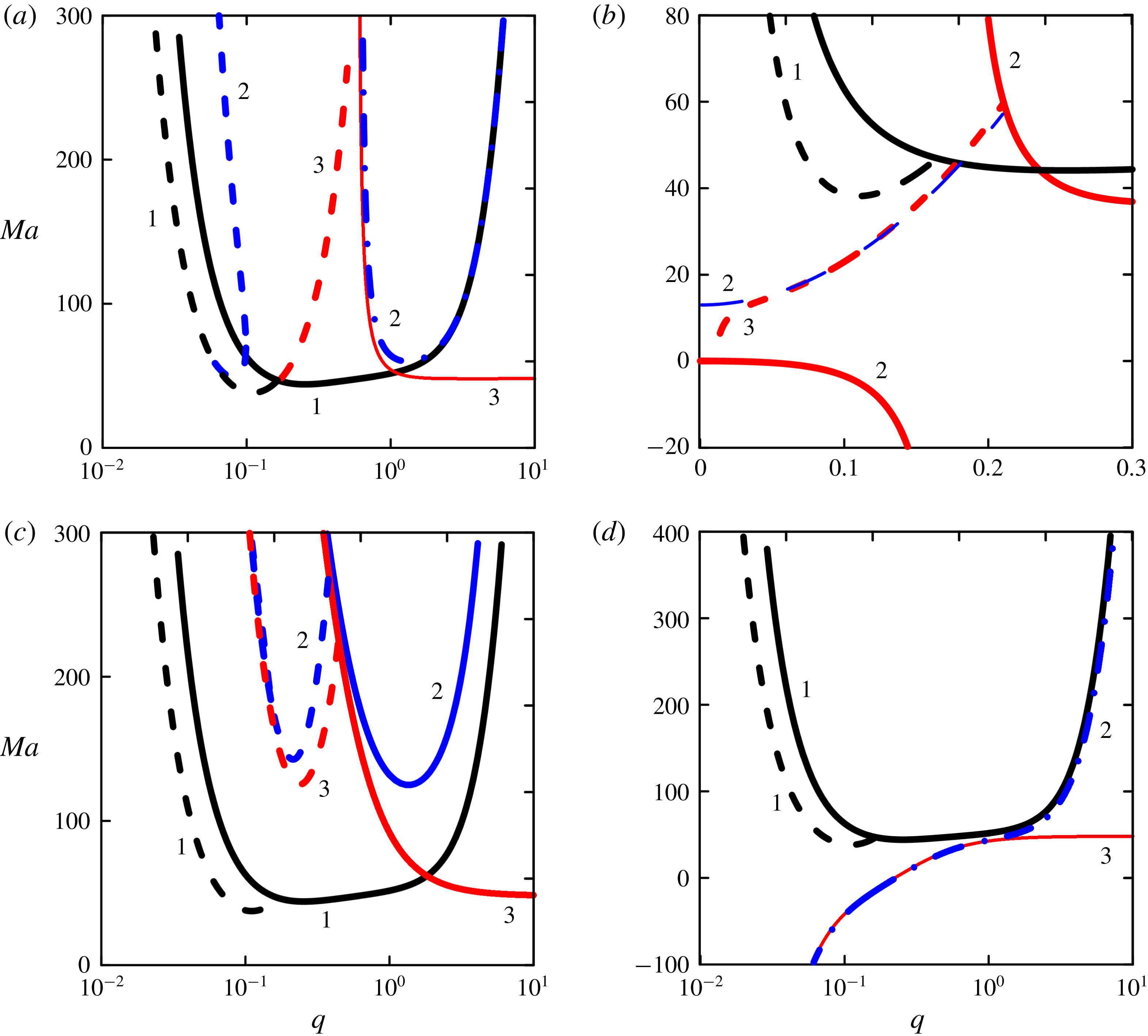
Neutral stability curves for the monotonic (solid and dashed-dotted lines) and the oscillatory (dashed lines) modes for control strategies (I) – panel (a), (IIa) – panel (b) and (IIb) – panels (c,d). Lines 1, 2 and 3 correspond to uncontrolled convection (
 $K_{s,Ts,T}=0$
), results for finite wavenumbers and to the long-wave asymptotic, respectively.
 $Pr=1$
,
 $Ga=10$
,
 $Ca=1000$
,
 $Bi=0.05$
. (a)
 $\text{K}_{s}~=2$
; (b)
 $K_{T}=0.05$
;(c)
 $K_{Ts}=-1$
; (d)
 $K_{Ts}=0.1$
.

Shklyaev et al. (Reference Shklyaev, Khenner and Alabuzhev2012) reported that the long-wave oscillatory mode is critical within the range where the capillary number is high and the Biot number is small, whereas their product is kept finite. As we focus on this particular mode of instability, we limit our calculations to the area of parameters where this oscillatory mode exists. Namely, we fix
 $Pr=1$
,
 $Ga=10$
,
 $Ca=1000$
,
 $Bi=0.05$
below. It should be pointed out that as we will compare the numerical results with the long-wave results from § 4, we need to match initial values of the parameters with their rescaled values. The expressions for the neutral stability curves within long-wave approximations (4.17)–(4.19), (4.22)–(4.26), (4.29) in terms of unscaled parameters remain the same if we replace
 $C\rightarrow Ca$
,
 $\unicode[STIX]{x1D6FD}\rightarrow Bi$
,
 $\unicode[STIX]{x1D718}_{s,Ts,T}\rightarrow K_{s,Ts,T}$
and
 $k\rightarrow q$
in them.
For the control strategy (I) the neutral stability curves for a small value of the control gain have no differences from those depicted in figure 1.
Moreover, the onset of the monotonic mode is captured nicely by the long-wave asymptotics even for finite values of
 $K_{s}$
. On the contrary, in the case of oscillatory instability the results for the finite positive values of
 $K_{s}$
reveal significant differences with the long-wave asymptotics.
As presented in figure 4(a), the oscillatory neutral curve goes up from the uncontrolled curve with the growth of the control gain, the onset of oscillatory mode moves to the long-wave area; monotonic and oscillatory branches are no longer connected. Thus, control strategy (I) with large positive values of the control gain can be used for stabilization of both modes of instability.
For the control strategy (IIa) all numerical results are in good qualitative agreement with the long-wave asymptotic that is presented in figure 2. The single neutral curve that is different from the long-wave prediction is depicted in figure 4(b): it is the oscillatory neutral curve for
 $K_{T}=Bi$
, which now is a line that connects two monotonic branches instead of the quadratic parabola in figure 2. Thus, it is confirmed by the linear analysis that for finite wavenumbers the given control technique is not appropriate to suppress the instability under consideration.
Numerical results for the control strategy (IIb) reveal considerable deviation from the long-wave asymptotic for finite positive and negative values of the control gain
 $K_{Ts}$
, see figure 4(c,d). In the case
 $K_{Ts}<0$
both monotonic and oscillatory neutral curves display much stronger suppression of the instability than it is predicted within the long-wave approach. In the case of
 $K_{Ts}>0$
the monotonic neutral curve has a form that is different from the long-wave neutral curve, as the latter tends to the Pearson limit
 $Ma=48$
.
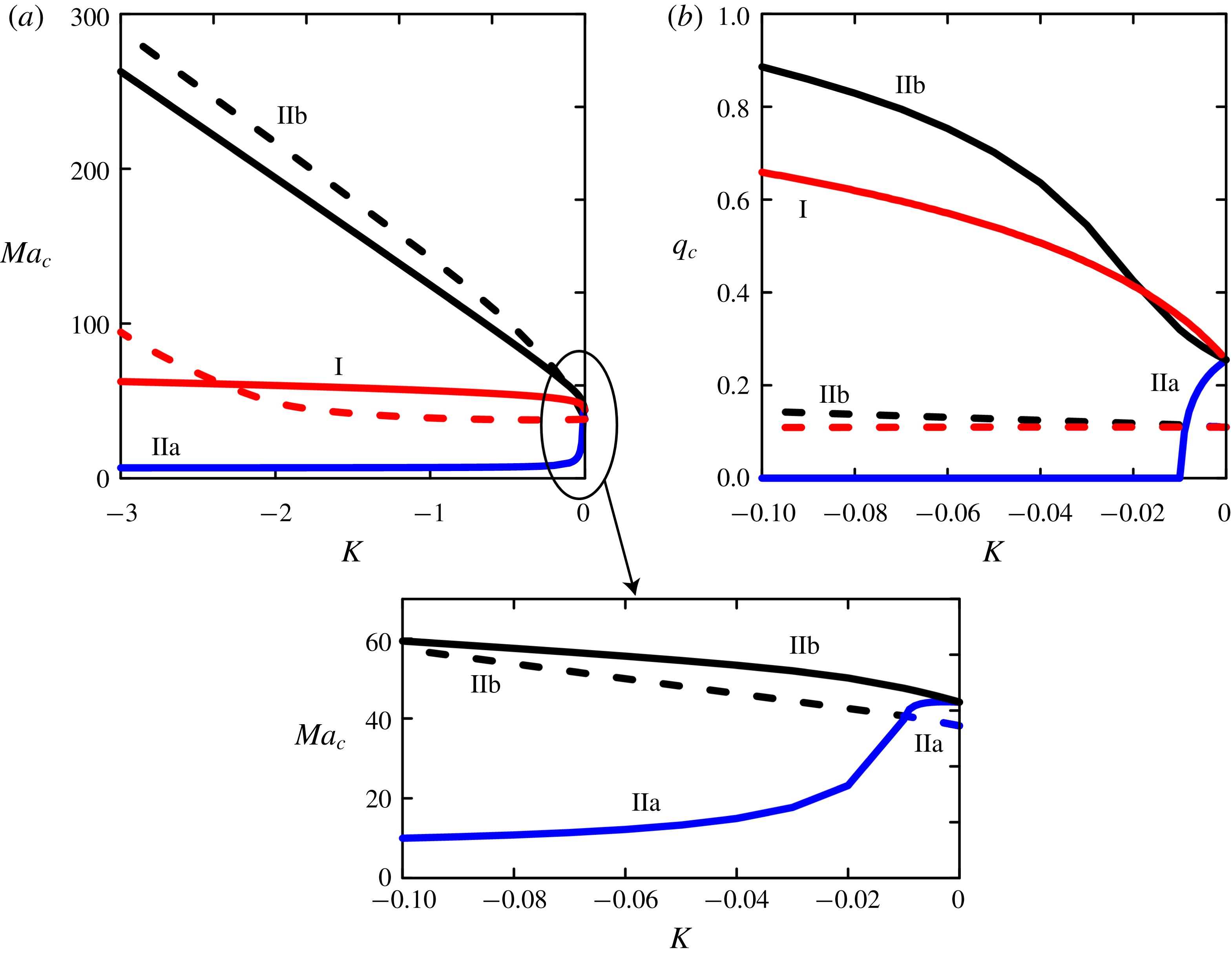
Aiming to find the most effective control strategy to suppress the Marangoni instability we provide a comparison of all three strategies investigated above. In figure 5 the results of neutral stability curve minimizations with respect to
 $q$
are juxtaposed for strategies (I), (IIa) and (IIb) within the wide range of control gain. Note that negative values of control gains
 $K_{T}$
and
 $K_{Ts}$
correspond to positive values of
 $K_{s}$
. Obviously, the control technique where the instability is detected by the departure of the surface fluid temperature from the conductive state is the most effective one to suppress the Marangoni convection in a thin film heated from below.
Comparison between three feedback control strategies. Variation of the critical Marangoni number (a) and the critical wavenumber (b) with the control gain
 $K$
, which denotes
 $-K_{s},K_{T}$
and
 $K_{Ts}$
for control strategies (I), (IIa) and (IIb), respectively. Dashed lines correspond to the oscillatory mode, solid lines correspond to the monotonic mode.
 $Pr=1$
,
 $Ga=10$
,
 $Ca=1000$
,
 $Bi=0.05$
.

6 Conclusion and discussion
The feedback control of the Marangoni instability in a thin film placed between its free deformable interface and a substrate of low heat conductivity is investigated.
The novelty of our investigation is in consideration of such physical conditions that the Marangoni convection in the thin film occurs through the oscillatory mode. The oscillatory instability in a thin film heated from below was revealed recently (Shklyaev et al. Reference Shklyaev, Khenner and Alabuzhev2012) through the coupling of two long-wave monotonic modes: Pearson’s mode (that requires a small heat flux from the free surface, i.e. small Biot number) and the deformational mode (that requires not too strong surface tension and gravity).
We applied linear feedback control to stabilize the no-motion state of a thin film heated from below in the situation where the oscillatory mode exists. Previously, the possibility of suppression of oscillatory Marangoni convection was demonstrated through the ‘open-loop’ control strategy (Shklyaev, Alabuzhev & Khenner Reference Shklyaev, Alabuzhev and Khenner2015). However, we suppose that the feedback control can be much more efficient, because it nearly vanishes when the desired state is achieved. We use two types of proportional linear feedback control, which show a good advantage in suppression of instabilities in large-aspect systems. The first one uses the free surface deflection from planarity as the measure of instability, the second one relies on the fluid temperature deviation from the conductive value.
Within the lubrication approximation, using scalings for the emergence of the oscillatory mode, we derive nonlinear amplitude equations, which describe the evolution of the thin film under different control strategies. Linear stability analysis of these amplitude equations provides the neutral stability curves for monotonic and oscillatory instabilities for a small control gain. This analysis was also extended to the case of finite wavenumbers and control gains.
Comparison of results for different control strategies reveals the most effective strategy to suppress the Marangoni instability in a thin film in the case when the oscillatory mode is critical. It is the strategy based on the deviation of free surface temperature from its conductive value. Note that previously, Bau (Reference Bau1999) showed that this strategy can be effective in suppressing the monotonic Marangoni instability. But in fact, Bau applied the strategy based on the deviation of the inner fluid temperature, as his model did not account for the free surface deformations. Within our investigation such a control strategy appears to be inefficient for suppression of the oscillatory instability, so we modified it to consider temperature perturbation together with free surface deflection from planarity. A simple explanation as to why this modified control strategy works better is the following. The oscillatory mode under consideration exists because of the coupling of two monotonic Marangoni modes: the Pearson and deformational modes, which are determined by the inhomogeneous temperature distribution on the deformed surface. Thus, changing the heat transfer from the deformed surface is the most effective way to govern this mode. Furthermore, within our model, temperature is not slaved to the interface position (see appendix A), so the control strategy based on the free surface position does not affect the oscillatory mode.
Speaking of possible experimental verification, we provide estimations for a realistic system. For a 0.1 mm film of silicone fluid of kinematic viscosity 100 cSt we obtain that the critical Marangoni number for uncontrolled oscillatory convection is attained at a temperature difference of 5 K. Applying the feedback control with controllers that measure free surface temperature (e.g. by infrared camera), one can delay the onset of convection until the boiling point of fluid.
Acknowledgement
This research was supported by the Israel Science Foundation (grant no. 843/18).
Appendix A.
Linear stability analysis of (4.8), (4.11) for normal perturbations
 $\unicode[STIX]{x0398}^{\prime }$
and
 $\unicode[STIX]{x1D701}$
provides the relation between the amplitudes of the perturbations
 $$\begin{eqnarray}\frac{\unicode[STIX]{x0398}_{m}^{\prime }}{\unicode[STIX]{x1D701}_{m}}=1-\frac{2}{3}\frac{G}{Ma}-\frac{2\unicode[STIX]{x1D706}}{k^{2}Ma},\end{eqnarray}$$
which remains the same for all three control strategies. Here
 $G=Ga+k^{2}C$
. Substituting formulas for the neutral stability curves
 $Ma^{m}$
and
 $Ma^{o}$
into this relation, we obtain for the monotonic mode
 $$\begin{eqnarray}\left.\begin{array}{@{}c@{}}\left({\displaystyle \frac{\unicode[STIX]{x0398}_{m}^{\prime }}{\unicode[STIX]{x1D701}_{m}}}\right)_{I}^{mon}=1-{\displaystyle \frac{k^{2}(72+G)-72\unicode[STIX]{x1D718}_{s}}{72(k^{2}+\unicode[STIX]{x1D6FD})}},\quad \left({\displaystyle \frac{\unicode[STIX]{x0398}_{m}^{\prime }}{\unicode[STIX]{x1D701}_{m}}}\right)_{IIa}^{mon}=1-{\displaystyle \frac{k^{2}\left(72+G\right)-72\unicode[STIX]{x1D718}_{T}}{72(k^{2}+\unicode[STIX]{x1D6FD}-\unicode[STIX]{x1D718}_{T})}},\\ \left({\displaystyle \frac{\unicode[STIX]{x0398}_{m}^{\prime }}{\unicode[STIX]{x1D701}_{m}}}\right)_{IIb}^{mon}=1-{\displaystyle \frac{k^{2}(72+G)}{72(k^{2}+\unicode[STIX]{x1D6FD}-\unicode[STIX]{x1D718}_{Ts})}},\end{array}\right\}\end{eqnarray}$$
and for the oscillatory mode
 $$\begin{eqnarray}\left(\frac{\unicode[STIX]{x0398}_{m}^{\prime }}{\unicode[STIX]{x1D701}_{m}}\right)_{I}^{osc}=\frac{k^{2}G+9(k^{2}+\unicode[STIX]{x1D6FD})-2\text{i}\unicode[STIX]{x1D714}_{I}}{3k^{2}G+9(k^{2}+\unicode[STIX]{x1D6FD})},\quad \left(\frac{\unicode[STIX]{x0398}_{m}^{\prime }}{\unicode[STIX]{x1D701}_{m}}\right)_{IIa}^{osc}=\frac{k^{2}G+9(k^{2}+\unicode[STIX]{x1D6FD}-\unicode[STIX]{x1D718}_{T})-2\text{i}\unicode[STIX]{x1D714}_{IIa}}{3k^{2}G+9(k^{2}+\unicode[STIX]{x1D6FD}-\unicode[STIX]{x1D718}_{T})}.\end{eqnarray}$$
For the control strategy II(b) the relation
 $(\unicode[STIX]{x0398}_{m}^{\prime }/\unicode[STIX]{x1D701}_{m})_{IIb}^{osc}$
is identical to
 $(\unicode[STIX]{x0398}_{m}^{\prime }/\unicode[STIX]{x1D701}_{m})_{IIa}^{osc}$
if we replace
 $\unicode[STIX]{x1D718}_{T}\rightarrow \unicode[STIX]{x1D718}_{Ts}$
and
 $\unicode[STIX]{x1D714}_{IIa}\rightarrow \unicode[STIX]{x1D714}_{IIb}$
. Expressions for the frequency of neutral perturbations
 $\unicode[STIX]{x1D714}_{I},\unicode[STIX]{x1D714}_{IIa}$
and
 $\unicode[STIX]{x1D714}_{IIb}$
are defined by (4.18), (4.23) and (4.14), respectively.
Appendix B.
For the monotonic mode (
 $\unicode[STIX]{x1D706}=0$
at the stability border) the boundary-value problem (5.5)–(5.8) has the following solution for all three control strategies
 $$\begin{eqnarray}\left.\begin{array}{@{}rcl@{}}W\,\, & =\,\, & C_{1}(\sinh qz-qz\cosh qz)+C_{2}qz\sinh qz,\\ \unicode[STIX]{x0398}\,\, & =\,\, & C_{3}\sinh qz+C_{4}\cosh qz+{\displaystyle \frac{C_{1}}{4q}}(qz^{2}\sinh qz-3z\cosh qz)\\ \,\, & \,\, & +\,{\displaystyle \frac{C_{2}}{4q}}(z\sinh qz-qz^{2}\cosh qz).\end{array}\right\}\end{eqnarray}$$
Here, the conditions at the lower boundary excepted for the control law, and the kinematic condition on the free surface have been applied. Substituting this solution into the conditions at the upper boundary and taking into account control laws (5.9), we obtain the expression that determines the neutral stability curve
 $$\begin{eqnarray}\displaystyle Ma_{I}^{m} & = & \displaystyle \frac{8qG(\cosh q\sinh q-q)(Bi\cosh q+q\sinh q)}{G(q^{2}\cosh q+\cosh q\sinh ^{2}q-2q\sinh q-q^{3}\sinh q)+8q^{5}\sinh q-8q^{4}K_{s}},\nonumber\\ \displaystyle & & \displaystyle\end{eqnarray}$$
 $$\begin{eqnarray}\displaystyle Ma_{IIa}^{m} & = & \displaystyle \frac{8G(\sinh q\cosh q-q)(qBi+q^{2}\sinh q+K_{T}(Bi\sinh q_{2}+q\cosh q_{2}))}{G(q^{2}\cosh q+\cosh q\sinh ^{2}q-q^{3}\sinh q-2q\sinh q)+8q^{5}\sinh q+8q^{4}K_{T}\unicode[STIX]{x1D6FE}},\nonumber\\ \displaystyle & & \displaystyle\end{eqnarray}$$
 $$\begin{eqnarray}\displaystyle \unicode[STIX]{x1D6FE} & = & \displaystyle \sinh q\sinh q_{2}-\cosh q\cosh q_{2}+G(\!4\sin \text{h}^{2}q(\cosh q\sinh q_{2}-\sinh q\cosh q_{2})\nonumber\\ \displaystyle & & \displaystyle +\,2q\sinh q\sinh q_{2}+q^{2}(6\cos \text{h}q\sinh q_{2}-5\sin \text{h}q\cosh q_{2})\nonumber\\ \displaystyle & & \displaystyle +\,3q^{3}(\cosh q\cosh q_{2}-\sinh q\sinh q_{2})\!)\!/32q^{5},\end{eqnarray}$$
 $$\begin{eqnarray}\displaystyle Ma_{IIb}^{m} & = & \displaystyle \frac{8qG(\cosh q\sinh q-q)(Bi\cosh q+q\sinh q-K_{Ts})}{G(q^{2}\cosh q+\cosh q\sinh ^{2}q-2q\sinh q-q^{3}\sinh q)+8q^{5}\sinh q},\end{eqnarray}$$
where
 $G=Ga+q^{2}Ca$
.
It can be shown that in the limit
 $q\rightarrow 0$
these equations become the asymptotic expressions of § 4.