1 Introduction
Sediment patterns, also commonly termed as dunes, ripples or simply bedforms, can be abundantly observed in deserts, coastal areas, natural streams or man-made canals. These sediment features, besides being simply fascinating, have important implications in many fields of science and engineering. For instance, bedforms greatly influence the rate of sediment transport as well as the stability of hydraulic structures in a given river. Thus, fundamental understanding of the mechanisms which are behind their formation as well as predicting their characteristics is crucial. However, this task has been very challenging due to the complex interaction between the sediment particles and the driving turbulent flow.
Sediment patterns in general can be broadly classified as ‘aeolian’ or ‘subaqueous’, the former being driven by wind forces while the latter, which the present study is focused on, form under water or due to the action of a similar fluid. The sediment-to-fluid density ratio of subaqueous patterns is much smaller than that of the aeolian ones. As a result, although the basic formation process is the same, there are fundamental differences regarding the relevant controlling mechanisms of their generation in both categories (cf. Bagnold Reference Bagnold1941; Sauermann, Kroy & Herrmann Reference Sauermann, Kroy and Herrmann2001; Andreotti & Claudin Reference Andreotti and Claudin2013; Duran, Claudin & Andreotti Reference Duran, Claudin and Andreotti2014).
Concerning subaqueous sediment patterns, one can further distinguish between those that form under the action of a steady flow, such as in rivers and canals, and those that are worked by an unsteady oscillatory flow, for instance by the action of a sea wave in coastal regions (cf. Sleath Reference Sleath1976; Blondeaux Reference Blondeaux1990; Vittori & Blondeaux Reference Vittori and Blondeaux1990; Blondeaux, Foti & Vittori Reference Blondeaux, Foti and Vittori2015). Henceforth we will restrict our attention to the study of patterns occurring in steady flows. Although subaqueous bedforms are three-dimensional objects, under certain circumstances they tend to be statistically invariant in the cross-stream direction (Yalin Reference Yalin1977). Indeed, a large part of the previous theoretical modelling and experimental measurement has focused on two-dimensional subaqueous bedforms (Best Reference Best2005), and this is the approach we take in the present work.
Bedforms can be characterized with respect to their spatial dimensions and their dynamics (Julien Reference Julien1998). Classically, a distinction is made between ripples, dunes and antidunes (Engelund & Fredsoe Reference Engelund and Fredsoe1982; García Reference García2008). Ripples and dunes exhibit some similarities, such as an asymmetric triangular-like shape with a gentle slope on the upstream side of their crest and a steeper slope on the downstream side. The principal distinction between ripples and dunes is the separation of length scales; the wavelength of observed ripples is commonly believed to scale with the grain size, and that of larger scale dunes is supposedly controlled by the flow geometry, typically the flow depth (Yalin Reference Yalin1977). Experiments show that at low flow rates small-scale undulations appear out of an initially flat sediment bed, at first having no clear-cut shape (Coleman & Melville Reference Coleman and Melville1994). When increasing the flow rate, these ripples give way to the much larger dunes, which are characterized by flow separation and recirculation in their downstream faces, and which propagate downstream. At even higher flow rates antidunes appear, which tend to propagate upstream. In the case of a flow with a free surface, both dunes and antidunes dynamically interact with surface waves (see e.g. Best Reference Best2005). Nevertheless, bedforms are equally observed in closed conduits which possess no free surface, and thus the existence of a free surface is not necessary for their formation (Yalin Reference Yalin1977; Bridge & Best Reference Bridge and Best1988; Langlois & Valance Reference Langlois and Valance2007; Ouriemi, Aussillous & Guazzelli Reference Ouriemi, Aussillous and Guazzelli2009; Cardona Florez & Franklin Reference Cardona Florez and Franklin2016). The problem of bedform and free surface wave interaction is not within the scope of the present study.
In most previous theoretical work on pattern formation, the background turbulent flow is typically represented by a Reynolds averaged Navier–Stokes equations (RANS) model, while the sediment-bed evolution is described by the sediment continuity equation, i.e. the Exner equation. The hydrodynamic and morphodynamic problems are then coupled by an algebraic expression for the particle flux as a function of the local bed shear stress. Hydro-morphodynamic linear (or weakly nonlinear) stability analysis is then performed in order to determine the stability of the sediment bed, the controlling parameter of the instability as well as the initial unstable pattern wavelength (e.g. see reviews by Seminara Reference Seminara2010; Charru, Andreotti & Claudin Reference Charru, Andreotti and Claudin2013). However, there is no clear consensus among the different predictions from these approaches, and, when compared to experimental observations, the outcome of these models is often unsatisfactory. For instance, the prediction for the initial pattern wavelength can be off by an order of magnitude (Raudkivi Reference Raudkivi1997; Langlois & Valance Reference Langlois and Valance2007; Coleman & Nikora Reference Coleman and Nikora2009a ; Ouriemi et al. Reference Ouriemi, Aussillous and Guazzelli2009). This inadequacy can be linked to, among others, the insufficient predictive capability of the adopted algebraic expressions for the particle flux.
The subsequent bedform evolution is an even more complicated issue which includes aspects like coarsening (bedform wavelength and amplitude growth), asymmetry, coalescence (fusion of bedforms), three-dimensional patterning (loss of bedform translational invariance). Even in simplified and controlled experiments where bedforms are essentially two-dimensional (see e.g. Betat et al. Reference Betat, Kruelle, Frette and Rehberg2002), the evolution process is a result of nonlinear interaction mechanisms which are far from our understanding. Certainly, linear stability theories are not adequate in describing the bedform transient processes such as the evolution of the amplitude or the evolution of bedform morphology towards the asymmetric shape (which is even observed in the absence of flow separation). Weakly nonlinear stability theories have been proposed (see e.g. Colombini & Stocchino Reference Colombini and Stocchino2008), but this approach is still unable to reliably predict the observed bedforms in reference experiments (e.g. Ouriemi et al. Reference Ouriemi, Aussillous and Guazzelli2009).
There exists a very limited amount of experimental studies available reporting on the initial formation and development stages of patterns (see e.g. Coleman & Melville Reference Coleman and Melville1994; Betat et al. Reference Betat, Kruelle, Frette and Rehberg2002; Coleman, Fedele & Garca Reference Coleman, Fedele and Garca2003; Langlois & Valance Reference Langlois and Valance2007; Ouriemi et al. Reference Ouriemi, Aussillous and Guazzelli2009; Cardona Florez & Franklin Reference Cardona Florez and Franklin2016). Even these studies, limited by measurement difficulties, often fall short of providing details with respect to the very first instants of the bed instability, such as the dispersion relation of the unstable modes. Such quantities are crucial when it comes to assessing the validity of the various proposed theoretical models. On the other hand, although there are a number of numerical studies available on the problem of subaqueous sedimentary patterns, most of these studies are based on the continuum description of the sediment bed, which again rely on the use of (semi-)empirical relationships to couple the hydro-morphodynamic problem (see e.g. Chou & Fringer Reference Chou and Fringer2010; Khosronejad & Sotiropoulos Reference Khosronejad and Sotiropoulos2014). In the granular flow community, a number of studies have been performed with the aid of a Lagrangian description of the sediment bed (based on discrete-element models), but without coupling to a resolved turbulent background flow (Durań, Andreotti & Claudin Reference Durań, Andreotti and Claudin2012; Schmeeckle Reference Schmeeckle2014; Maurin et al. Reference Maurin, Chauchat, Chareyre and Frey2015).
There has been a promising gain of momentum in recent years on the number of direct numerical simulation (DNS) studies on the problem of sediment transport in which the detail of the flow, even at the boundaries of each individual particles, is faithfully resolved (see e.g. Kidanemariam & Uhlmann Reference Kidanemariam and Uhlmann2014a
; Kidanemariam & Uhlmann Reference Kidanemariam and Uhlmann2014
b
; Vowinckel, Kempe & Fröhlich Reference Vowinckel, Kempe and Fröhlich2014; Derksen Reference Derksen2015). We have recently performed novel DNS of the flow over an erodible bed of spherical sediment particles in a statistically unidirectional channel flow configuration in both the laminar and turbulent regimes (Kidanemariam & Uhlmann Reference Kidanemariam and Uhlmann2014a
). These simulations are, to the best of our knowledge, the first to successfully simulate the evolution of a bed of mobile sediment particles (leading to pattern formation) by means of DNS (Colombini Reference Colombini2014). The results from these simulations have shown that the chosen streamwise length of the computational domain (
 $12H_{f}$
, where
 $H_{f}$
is the channel fluid height) was able to accommodate a few integer multiples of the initial pattern wavelength, which allowed us to address some of the outstanding questions on sedimentary patterns such as the initial dominant wavelength and pattern amplitude growth (Kidanemariam & Uhlmann Reference Kidanemariam and Uhlmann2014a
). Ideally, in order to accurately capture the natural selection mechanism of the unstable wavelength and its subsequent evolution, it is necessary to consider a computational domain size which is much greater than the anticipated pattern wavelength. However, the domain sizes considered by Kidanemariam & Uhlmann (Reference Kidanemariam and Uhlmann2014a
) might be marginal when compared to the observed dominant wavelengths. It was noted that the discreteness of the numerical harmonics could influence the initial wavelength as well as the time evolution processes. In light of this aspect, assessing the influence of the domain size on the selection and evolution process is crucial.
Moreover, various theoretical and experimental studies have shown that there is a lower threshold of the unstable wavelengths (see for instance Charru Reference Charru2006; Franklin & Charru Reference Franklin and Charru2011). Determination of this value is important, since the lower bound of unstable modes is believed to be linked to some relevant length scale which controls erodible bed instability (Hersen, Douady & Andreotti Reference Hersen, Douady and Andreotti2002; Claudin & Andreotti Reference Claudin and Andreotti2006; Andreotti et al. Reference Andreotti, Claudin, Devauchelle, Durán and Fourrière2011).
In the present work, we have carried out a series of simulations of the same flow configuration as in our previous study (Kidanemariam & Uhlmann Reference Kidanemariam and Uhlmann2014a
). We have kept all the physical and numerical parameters of the simulations identical, except for the streamwise length of the computational box. The latter was varied between
 $3H_{f}$
and
 $48H_{f}$
, in order to determine whether at the considered parameter point there exists a cutoff length for pattern formation. To this end, we have successively reduced the domain size until it is smaller than an unknown threshold and cannot accommodate an unstable bed. Moreover, in order to assess the influence of the domain size on the selection of the initial ripple wavelength and its subsequent evolution, we have chosen a computational domain size which is four times larger than in our previous study. It should be noted that a very large number of spherical particles (approximately 1.1 million in total) are considered to represent the mobile bed. This simulation is the first of its kind to break the
 $O(10^{6})$
fully resolved particle milestone. Furthermore, based on the analysis of the DNS data, we address the relationship between the evolving patterns, their migration velocity and the particle flow rate at the present parameter point.
2 Numerical method
In the present work we have used the same numerical procedure as Kidanemariam & Uhlmann (Reference Kidanemariam and Uhlmann2014a
), Kidanemariam & Uhlmann (Reference Kidanemariam and Uhlmann2014
b
). The numerical treatment of the fluid–solid system is based upon the immersed boundary technique of Uhlmann (Reference Uhlmann2005), wherein the incompressible Navier–Stokes equations are solved with a second-order finite-difference method throughout the entire computational domain, adding a localized force term which serves to impose the no-slip condition at the fluid–solid interface. The particle motion is obtained via integration of the Newton–Euler equations for rigid body motion, driven by the hydrodynamic force (and torque) as well as gravity and the force (torque) resulting from solid–solid contact. The collision process between the immersed particles is described through a discrete-element model (DEM) based on the soft-sphere approach. A pair of particles is defined as ‘being in contact’ when the smallest distance between their surfaces,
 $\unicode[STIX]{x1D6E5}$
, becomes smaller than a force range
 $\unicode[STIX]{x1D6E5}_{c}$
. The resulting contact force is then the sum of an elastic normal component, a normal damping component and a tangential frictional component. The elastic part of the normal force component is a linear function of the penetration length
 $\unicode[STIX]{x1D6FF}_{c}\equiv \unicode[STIX]{x1D6E5}_{c}-\unicode[STIX]{x1D6E5}$
, with a stiffness constant
 $k_{n}$
. The normal damping force is a linear function of the normal component of the relative velocity between the particles at the contact point with a constant coefficient
 $c_{n}$
. The tangential frictional force (the magnitude of which is limited by the Coulomb friction limit with a friction coefficient
 $\unicode[STIX]{x1D707}_{c}$
) is a linear function of the tangential relative velocity at the contact point, again formulated with a constant coefficient denoted as
 $c_{t}$
. A detailed description of the collision model and extensive validation can be found in Kidanemariam & Uhlmann (Reference Kidanemariam and Uhlmann2014
b
).
The four parameters which describe the collision process in the framework of this model (
 $k_{n}$
,
 $c_{n}$
,
 $c_{t}$
,
 $\unicode[STIX]{x1D707}_{c}$
) as well as the force range
 $\unicode[STIX]{x1D6E5}_{c}$
need to be prescribed for each simulation. Note that the normal stiffness coefficient
 $k_{n}$
and the normal damping coefficient
 $c_{n}$
can be related by introducing the dry restitution coefficient
 $\unicode[STIX]{x1D700}_{d}$
, defined as the absolute value of the ratio between the normal components of the relative velocity post-collision and pre-collision.
In the present simulations,
 $\unicode[STIX]{x1D6E5}_{c}$
is set equal to one grid spacing
 $\unicode[STIX]{x0394}x$
. The stiffness parameter
 $k_{n}$
has a value equivalent to approximately 17 000 times the submerged weight of the particles, divided by the particle diameter. The chosen value ensures that the maximum overlap
 $\unicode[STIX]{x1D6FF}_{c}$
over all contacting particle pairs is within a few percent of
 $\unicode[STIX]{x1D6E5}_{c}$
. The dry coefficient of restitution is set to
 $\unicode[STIX]{x1D700}_{d}=0.3$
, which together with
 $k_{n}$
fixes the value for
 $c_{n}$
. Finally, the tangential damping coefficient
 $c_{t}$
was set equal to
 $c_{n}$
, and a value of
 $\unicode[STIX]{x1D707}_{c}=0.4$
was imposed for the Coulomb friction coefficient. This set of parameter values for the contact model is the same as used by Kidanemariam & Uhlmann (Reference Kidanemariam and Uhlmann2014
b
).
Since the characteristic collision time is typically orders of magnitude smaller than the time step of the flow solver, the numerical integration of the equations for the particle motion is carried out adopting a sub-stepping technique, freezing the hydrodynamic forces acting upon the particles between successive flow-field updates (Kidanemariam Reference Kidanemariam2015).
3 Flow configuration and parameter values
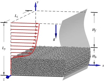
We have performed a total of ten independent simulations of the development of bedforms over a subaqueous sediment in an open channel flow configuration. As shown in figure 1 a Cartesian coordinate system is adopted such that
 $x$
,
 $y$
, and
 $z$
are the streamwise, wall-normal and spanwise directions, respectively. Mean flow and gravity are directed in the positive
 $x$
and the negative
 $y$
directions respectively. The computational domain is periodic in the streamwise and spanwise directions. A free-slip condition is imposed at the top boundary while a no-slip condition is imposed at the bottom wall. The simulations are labelled H3, H4, H6, H7, H12 and H48, indicating the approximate streamwise box length in terms of the mean fluid height
 $H_{f}$
. The mean fluid height
 $H_{f}$
and the corresponding mean sediment-bed thickness
 $H_{b}$
are computed by performing streamwise and time averaging of the spanwise-averaged instantaneous fluid height
 $h_{f}$
and sediment-bed height
 $h_{b}$
(note that the definition of
 $h_{f}$
and
 $h_{b}$
will be made more precise in § 4.1). In order to perform ensemble averaging, case H4 and H12 are performed three times, each adopting different initial conditions. Each simulation is performed independently following the simulation start-up procedure as detailed in Kidanemariam & Uhlmann (Reference Kidanemariam and Uhlmann2014a
).
Schematic diagram showing the configuration of the simulations. The computational domain is periodic along the
 $x$
- and
 $z$
-directions. The no-slip and free-slip boundary conditions are imposed at the bottom (
 $y=0$
) and top (
 $y=L_{y}$
) respectively.

In all cases, the channel is driven by a horizontal mean pressure gradient which is adjusted at each time step in order to impose a constant flow rate
 $q_{f}$
. This results in a shearing flow of fluid height
 $H_{f}$
over a mobile bed of height
 $H_{b}$
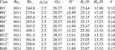
(cf. sketch in figure 1). As is shown in table 1, the bulk Reynolds number of the flow, which is defined based on the mean height of the fluid as
 $$\begin{eqnarray}Re_{b}=\frac{u_{b}H_{f}}{\unicode[STIX]{x1D708}},\end{eqnarray}$$
where
 $u_{b}\equiv q_{f}/H_{f}$
is the bulk velocity and
 $\unicode[STIX]{x1D708}$
is the kinematic viscosity, is set at a value such that the flow is fully turbulent. The friction Reynolds number
 $Re_{\unicode[STIX]{x1D70F}}$
, which is similarly defined based on the friction velocity
 $u_{\unicode[STIX]{x1D70F}}$
, is a posteriori determined by evaluating the total shear stress at the wall-normal location of the mean fluid–bed interface
 $y=H_{b}$
(cf. § 5.4 for details of the determination of
 $u_{\unicode[STIX]{x1D70F}}$
).
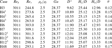
Physical parameters of the simulations. In all cases, the values of the bulk Reynolds number
 $Re_{b}$
, the particle-to-fluid density ratio
 $\unicode[STIX]{x1D70C}_{p}/\unicode[STIX]{x1D70C}_{f}$
and the Galileo number
 $Ga$
are imposed. Derived physical parameters include the friction Reynolds number
 $Re_{\unicode[STIX]{x1D70F}}$
, the Shields number
 $\unicode[STIX]{x1D703}$
as well as the length-scale ratios
 $H_{f}/D$
,
 $H_{b}/D$
and
 $D^{+}$
. Note that three independent simulations are performed for cases H4 and H12 each for the purpose of ensemble averaging. The values of the relevant parameters are determined over a time interval at the end of the respective simulations (cf. table 2).
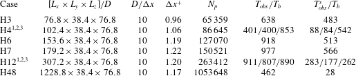
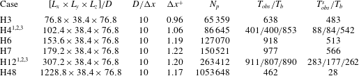
Numerical parameters of the simulations.
 $L_{i}$
is the domain length adopted in the
 $i\text{th}$
direction. In all the cases, the spherical particles have a diameter
 $D=10/256$
and a uniform grid spacing
 $\unicode[STIX]{x0394}x=\unicode[STIX]{x0394}y=\unicode[STIX]{x0394}z=1/256$
is adopted yielding the above listed resolutions.
 $N_{p}$
is the number of spherical particles adopted.
 $T_{obs}$
is the total simulation time interval staring from the instant at which the mobile particles are released, while
 $T_{obs}^{s}$
corresponds to the interval (at the end of the respective simulations) during which statistical averaging is performed to determine the relevant parameters listed in table 1 (
 $Re_{\unicode[STIX]{x1D70F}}$
,
 $D^{+}$
,
 $H_{b}/D$
, and
 $\unicode[STIX]{x1D703}$
) and to compute steady-state ripple quantities which are discussed in §§ 5.2, 5.3, 5.4 and 5.5.
 $T_{b}\equiv H_{f}/u_{b}$
is the bulk time unit.
In order to fully describe the flow, at least three parameters in addition to
 $Re_{b}$
need to be imposed: the particle-to-fluid density ratio
 $\unicode[STIX]{x1D70C}_{p}/\unicode[STIX]{x1D70C}_{f}$
, a length-scale ratio
 $H_{f}/D$
, and a ratio between the gravity and viscous forces which is described by the Galileo number viz.
 $$\begin{eqnarray}Ga=\frac{((\unicode[STIX]{x1D70C}_{p}/\unicode[STIX]{x1D70C}_{f}-1)|\boldsymbol{g}|D^{3})^{1/2}}{\unicode[STIX]{x1D708}}=\frac{U_{g}D}{\unicode[STIX]{x1D708}},\end{eqnarray}$$
where
 $g$
is the gravitational acceleration.
 $Ga$
can be considered as a Reynolds number defined based on the gravitational velocity scale
 $U_{g}=\sqrt{(\unicode[STIX]{x1D70C}_{p}/\unicode[STIX]{x1D70C}_{f}-1)|\boldsymbol{g}|D}$
and the particle diameter. Note that
 $U_{g}$
is not the actual settling velocity (Jenny, Dušek & Bouchet Reference Jenny, Dušek and Bouchet2004). The density ratio is fixed at a value of
 $\unicode[STIX]{x1D70C}_{p}/\unicode[STIX]{x1D70C}_{f}=2.5$
, which corresponds to the density ratio between glass beads and water. The thickness of the fluid height and that of the erodible bed are chosen to be sufficiently large for the formation of the anticipated bed patterns. This results in a very large number of spherical particles due to the size the computational box (cf. table 2). Finally, the value of the Galileo number is chosen by adjusting the value of acceleration due to gravity
 $|\boldsymbol{g}|$
, such that the value of the Shields number
 $$\begin{eqnarray}\unicode[STIX]{x1D703}=\frac{u_{\unicode[STIX]{x1D70F}}^{2}}{\left(\unicode[STIX]{x1D70C}_{p}/\unicode[STIX]{x1D70C}_{f}-1\right)|\boldsymbol{g}|D}=\frac{u_{\unicode[STIX]{x1D70F}}^{2}}{U_{g}^{2}}=\left(\frac{D^{+}}{Ga}\right)^{2},\end{eqnarray}$$
is above the critical value
 $\unicode[STIX]{x1D703}_{c}$
for incipient sediment motion. In the turbulent flow regime,
 $\unicode[STIX]{x1D703}_{c}$
is believed to approximately lie in the range
 $0.03\ldots 0.05$
, with a mild dependence upon the Galileo number (Soulsby & Whitehouse Reference Soulsby and Whitehouse1997; Wong & Parker Reference Wong and Parker2006; Franklin & Charru Reference Franklin and Charru2011).
We remark that the present parameter point is located in the ‘vortex dune’ regime in the classification of Ouriemi et al. (Reference Ouriemi, Aussillous and Guazzelli2009). These authors coined the term ‘vortex dunes’ for patterns which are characterized by flow separation and recirculation at their downstream face, in order to distinguish them from smaller-amplitude patterns without flow separation which they observed in their pipe-flow experiments (the latter were termed ‘small dunes’ therein). Note that this terminology should not be confused with the distinction between ‘ripples’ and ‘dunes’ commonly made in the river flow community; in particular, it does not imply that the length scales of the present patterns exhibit a scaling with the water depth.
Incidentally, let us mention that the chosen parameters of our simulation can be transformed into a physically realizable laboratory experiment. For instance, choosing as working fluid a mixture of 94 % pure water and 6 % UCON oil 75H-90 000 (leading to kinematic viscosity of the mixture of
 $4.3\times 10^{-6}~\text{m}^{2}~\text{s}^{-1}$
and a mixture density of
 $1002~\text{kg}~\text{m}^{-3}$
), and selecting
 $D=1~\text{mm}$
glass beads implies the following dimensions of the experimental apparatus (under terrestrial conditions): channel height 3.9 cm, fluid height 2.5 cm, wavelength of obtained ripples in the range of
 $10{-}18~\text{cm}$
. The bulk velocity in this hypothetical set-up would measure
 $0.52~\text{m}~\text{s}^{-1}$
.
4 Extraction of bedform dimensions
4.1 Definition of the fluid–bed interface
The details of the extraction of the fluid–bed interface, which have been given in our previous work (Kidanemariam & Uhlmann Reference Kidanemariam and Uhlmann2014a
; Kidanemariam Reference Kidanemariam2015), are briefly repeated here for completeness. The location of the interface between the fluid and the sediment bed has been determined based on the threshold value of the solid volume fraction in the following way. First, a solid phase indicator function
 $\unicode[STIX]{x1D719}_{p}(\boldsymbol{x},t)$
is defined which has a value of one if
 $\boldsymbol{x}$
is located inside any particle and zero elsewhere. Spanwise averaging then yields
 $\langle \unicode[STIX]{x1D719}_{p}\rangle _{z}(x,y,t)$
, which is a direct measure of the instantaneous, two-dimensional solid volume fraction. The spanwise-averaged fluid–bed interface location
 $h_{b}(x,t)$
is finally extracted by means of a threshold value, chosen as
 $\langle \unicode[STIX]{x1D719}_{p}\rangle _{z}^{thresh}=0.1$
(Kidanemariam & Uhlmann Reference Kidanemariam and Uhlmann2014
b
), viz.
 $$\begin{eqnarray}h_{b}(x,t)=y\;|\;\langle \unicode[STIX]{x1D719}_{p}\rangle _{z}(x,y,t)=\langle \unicode[STIX]{x1D719}_{p}\rangle _{z}^{thresh}.\end{eqnarray}$$
The corresponding spanwise-averaged fluid height is then simply given by
 $$\begin{eqnarray}h_{f}(x,t)=L_{y}-h_{b}(x,t).\end{eqnarray}$$
In the present study, we infer the evolution of the dimensions of the patterns as well as their two-dimensional shape and propagation velocity by scrutinizing the spatial and temporal variation of the sediment-bed height
 $h_{b}$
or its fluctuation with respect to the instantaneous average bed height,
 $$\begin{eqnarray}h_{b}^{\prime }(x,t)=h_{b}(x,t)-\langle h_{b}\rangle _{x}(t).\end{eqnarray}$$
4.2 Definition of pattern amplitude and wavelength
The most relevant parameters, among others, which describe the geometrical features of statistically two-dimensional bedforms are their streamwise and wall-normal dimensions, namely the mean wavelength and mean amplitude of the patterns. As reviewed by Coleman & Nikora (Reference Coleman and Nikora2011), various definitions have been used in order to quantify these dimensions. For instance, the average wall-normal distance between local maxima and adjacent local minima of
 $h_{b}$
is used as a measure of the amplitude of the patterns in some studies (Ouriemi et al.
Reference Ouriemi, Aussillous and Guazzelli2009). Other studies infer the amplitude of the patterns statistically from the r.m.s. fluctuation of the bed (Langlois & Valance Reference Langlois and Valance2007). Similarly, the wavelength of patterns is quantified either geometrically, for instance based on the mean spacing between alternating troughs or ridges of the sediment-bed height, or statistically, for instance based on the autocorrelation of the bed-height fluctuation (Coleman & Nikora Reference Coleman and Nikora2011). In the present study, we have adopted a statistical definition.
The wall-normal dimension of the patterns is characterized by the r.m.s. fluctuation of the sediment bed
 $\unicode[STIX]{x1D70E}_{h}$
, defined as
 $$\begin{eqnarray}\unicode[STIX]{x1D70E}_{h}^{2}(t)=\langle h_{b}^{\prime }(x,t)\cdot h_{b}^{\prime }(x,t)\rangle _{x}.\end{eqnarray}$$
In order to determine the average wavelength of the patterns, first we define the instantaneous two-point correlation coefficient of the bed-height fluctuation as a function of streamwise separation
 $\unicode[STIX]{x1D6FF}x$
as
 $$\begin{eqnarray}R_{h}(\unicode[STIX]{x1D6FF}x,t)=\frac{\langle h_{b}^{\prime }(x,t)\cdot h_{b}^{\prime }(x+\unicode[STIX]{x1D6FF}x,t)\rangle _{x}}{\unicode[STIX]{x1D70E}_{h}^{2}(t)}.\end{eqnarray}$$
At a given time instant
 $t=t_{1}$
, the correlation coefficient
 $R_{h}(\unicode[STIX]{x1D6FF}x,t_{1})$
of a sediment bed featuring bedforms, exhibits a distinct damped-oscillation curve featuring alternating positive and negative values as a function of
 $\unicode[STIX]{x1D6FF}x$
. Then, we define an average bedform wavelength
 $\unicode[STIX]{x1D706}_{h}$
as twice the streamwise separation
 $\unicode[STIX]{x1D6FF}x=x_{min}$
at which the global minimum of
 $R_{h}$
occurs viz.
 $$\begin{eqnarray}\unicode[STIX]{x1D706}_{h}(t)=2x_{min}\;|\;\forall \,\unicode[STIX]{x1D6FF}x\in [0,\,L_{x}/2]:R_{h}(\unicode[STIX]{x1D6FF}x,t)\geqslant R_{h}(x_{min},t).\end{eqnarray}$$
5 Results
During the preparation of the present manuscript we have discovered a programming error in the solid contact part of the simulation code. This bug was active during the simulations of Kidanemariam & Uhlmann (Reference Kidanemariam and Uhlmann2014a ). After correcting the error, we have rerun those simulations and compared the results. This comparison is discussed in the Appendix. The conclusion from this assessment is that the results did not change qualitatively. Concerning the quantitative comparison, it can be stated that the difference between the result with and without bug is within the scatter due to the three independent realizations simulated here.
5.1 The minimum and the most amplified unstable pattern wavelengths
Our strategy to find the minimal box length
 $L_{x}$
which will accommodate the lower bound of the unstable wavelengths
 $\unicode[STIX]{x1D706}_{th}$
(at a given parameter point) is to perform a series of numerical experiments in which the streamwise domain length is successively reduced. The concept is similar to the minimal flow unit of Jiménez & Moin (Reference Jiménez and Moin1991). Below a threshold value of
 $L_{x}=\unicode[STIX]{x1D706}_{th}$
, pattern evolution will be hindered and a perturbed bed should in principle be stable even though it is in a regime where instability is expected. Note that determining the lower threshold of
 $\unicode[STIX]{x1D706}_{th}$
for bed instability does not necessarily mean determining the most amplified wavelength
 $\unicode[STIX]{x1D706}_{c}$
. The latter, if it uniquely exists, exhibits the maximum growth rate of the bed instability.
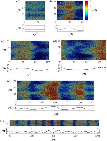
Figure 2 shows instantaneous snapshots of the particle positions in the different cases after approximately 200 bulk time units have elapsed. It can be seen that the sediment bed of case H3 does not feature dune-like patterns. However, one can observe that it exhibits distinct streamwise aligned alternating ridges and troughs, although the sediment bed is essentially flat when the spanwise average of the sediment-bed profile is observed. Such an organization of particles is linked to the streamwise-aligned near-wall turbulent structures (streaks) which are responsible for the non-homogeneous spatial distribution of particles. The highly regular ridge-trough pattern in this case is a result of the very small box length which hinders spatial de-correlation of the turbulent structures in the streamwise direction. On the other hand, the sediment bed of the remaining cases with
 $L_{x}\geqslant 4H_{f}$
is seen to be unstable, allowing for the formation of spanwise-oriented patterns. The streamwise-aligned patterns are also visible superimposed to the ripples (in the remainder of the present text we will refer to the observed bedforms as ripples). This indicates that the value of
 $\unicode[STIX]{x1D706}_{th}$
lies somewhere between the domain lengths of cases H3 and H4. Another observation is that the initial wavelength of the emerging patterns seems to be different depending on the chosen domain length. In particular, the case with the largest domain size, which has a streamwise box length 12 times the smallest domain length of the ripple-featuring cases, is observed to accommodate more than ten initial ripple units. The dimension of the ripples in the large domain case seems to have evolved less constrained by the box size when compared to those in the small domain cases. Let us provide a more quantitative analysis of the above observation by evaluating the r.m.s. sediment-bed-height fluctuation
 $\unicode[STIX]{x1D70E}_{h}$
of each case and using it as a criterion to determine whether a sediment bed in a given simulation is stable or not. That is, if
 $\unicode[STIX]{x1D70E}_{h}$
remains bounded within a certain threshold value, then the bed is said to be stable. On the other hand, for an unstable bed,
 $\unicode[STIX]{x1D70E}_{h}$
will initially exhibit a continuous increase as a function of time. Note that even a stable flat (mobile) sediment bed features a small but finite value of
 $\unicode[STIX]{x1D70E}_{h}$
as a result of the random uncorrelated bed undulations which stem from the discreteness of the bed at the grain scale. For instance, Coleman & Nikora (Reference Coleman and Nikora2009a
) report
 $\unicode[STIX]{x1D70E}_{h}/D\approx 0.17$
for their macroscopically ‘flat’ bed.
Top view of the three-dimensional instantaneous particle positions and the corresponding spanwise-averaged fluid–bed interface (shown below each snapshot) at time
 $t/T_{b}\approx 200$
of cases (a) H3, (b) H4, (c) H6, (d) H7, (e) H12 and (f) H48. The wall-normal particle location is indicated by a global colour code, as shown in (b).

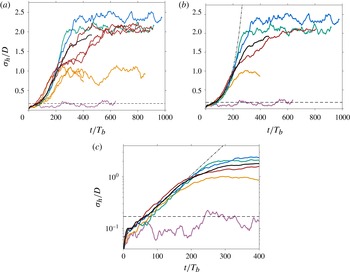
(a) Time evolution of the r.m.s. sediment-bed-height fluctuation normalized by the particle diameter: — (purple), case H3; — (orange), case H4; — (green), case H6; — (blue), case H7; — (brown), case H12; —, case H48. The horizontal dashed line indicates the value
 $\unicode[STIX]{x1D70E}_{h}/D\approx 0.17$
which corresponds to the random bed fluctuations of featureless flat bed (Coleman & Nikora Reference Coleman and Nikora2009a
). (b) Same as in (a) but the data for cases H4 and H12 are ensemble averaged over the number of simulations performed. The dashed-dot line corresponds to an exponential fit curve
 $\unicode[STIX]{x1D70E}_{h}/D=0.0668\exp (0.0140t/T_{b})$
obtained from an average amplitude growth in the initial exponential interval. (c) Same as in (b) but plotted in log-linear scale to highlight the exponential growth regime during the first instant of the bed instability.

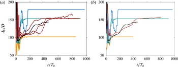
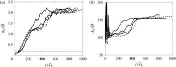
(a) Time evolution of the mean wavelength
 $\unicode[STIX]{x1D706}_{h}$
of the sediment-bed height normalized by the particle diameter. Colour coding similar to figure 3. (b) The same as in (a) but the data for cases H4 and H12 are ensemble averaged over the number of simulations performed.

Figure 3 shows the time evolution of
 $\unicode[STIX]{x1D70E}_{h}$
for all the considered cases listed in table 1. It is seen that, starting from time
 $tu_{b}/H_{f}\approx 20$
, the value of
 $\unicode[STIX]{x1D70E}_{h}$
grows with time for all the cases with domain length
 $L_{x}\geqslant 102.4D$
(
 $L_{x}\geqslant 4H_{f}$
), indicating that the chosen streamwise box dimension of these cases is larger than the lower threshold of unstable wavelengths, such that the box can accommodate at least one of the unstable modes. On the contrary, the evolution of
 $\unicode[STIX]{x1D70E}_{h}$
in case H3 exhibits no growth with time except for small fluctuations;
 $\unicode[STIX]{x1D70E}_{h}$
in this case is effectively bounded by the threshold value
 $\unicode[STIX]{x1D70E}_{h}/D\approx 0.17$
as per Coleman & Nikora (Reference Coleman and Nikora2009a
). This indicates that the streamwise box length
 $L_{x}=76.8D$
(
 $L_{x}=3H_{f}$
) is not sufficient to accommodate the lower threshold of unstable modes. Thus, it can be concluded that a cutoff length scale for pattern formation (for the considered parameter point) lies in the range
 $77D<\unicode[STIX]{x1D706}_{th}<102D$
, or in terms of the mean fluid height,
 $3H_{f}<\unicode[STIX]{x1D706}_{th}<4H_{f}$
. Additional simulations with
 $L_{x}$
in the range
 $3H_{f}$
to
 $4H_{f}$
would be required in order to determine
 $\unicode[STIX]{x1D706}_{th}$
more accurately.
Furthermore, figure 3 highlights the fact that the evolution of the pattern amplitude exhibits distinct regimes of growth. During the first approximately 150 to 180 bulk time units (excluding the first of approximately 20 bulk time units during which the sediment bed initially dilates after the start of the simulations),
 $\unicode[STIX]{x1D70E}_{h}$
is observed to evolve exponentially for all the cases, with a growth rate which seems to be independent of the chosen domain size. Note that the time evolution of
 $\unicode[STIX]{x1D70E}_{h}$
for cases H4 and H12 presented in figure 3(b,c) is an ensemble average over the three separate simulations of the respective cases. An exponential curve of the form
 $$\begin{eqnarray}\unicode[STIX]{x1D70E}_{h}/D=A\exp (Bt/T_{b}),\end{eqnarray}$$
with
 $A=0.0668$
and
 $B=0.0140$
, best fits the average growth over all cases in this interval. In the subsequent growth regime, the trend of the amplitude evolution is observed to be markedly different among the different cases, although all were carried out at the same imposed parameter values. After the initial exponential growth (up to
 $t\approx 200T_{b}$
), and after a small transition interval of approximately
 $100T_{b}$
, cases H4, H6 and H7 exhibit a plateau of the pattern amplitude, showing no further growth with time. The attained final values are
 $\unicode[STIX]{x1D70E}_{h}/D=0.93$
,
 $2.08$
and
 $2.36$
for each of these cases, respectively. The evolution of
 $\unicode[STIX]{x1D70E}_{h}$
for case H12 also attains a plateau regime with a final value of
 $\unicode[STIX]{x1D70E}_{h}$
comparable to that of case H6. However, it settles to this value not immediately after the exponential regime, rather it gradually increases (approximately linearly) in the interval between
 $t=200T_{b}$
and
 $600T_{b}$
. On the other hand, since the observation interval of case H48 is shorter, it has covered only the exponential growth regime by the end of the simulation.
The different trend of the amplitude growth observed is closely related to the influence of the limited computational box size on the initially accommodated mean wavelength and its subsequent evolution. In cases H4, H6, H7 and H12, even though the streamwise length of the computational box is larger than the threshold for pattern formation, due to the fact that
 $L_{x}/\unicode[STIX]{x1D706}_{th}=O(1)$
, the discrete wavelengths from which the system has to select are very sparse, and it is not guaranteed that the initially selected wavelength will be the same as the one which an infinitely long system would select. On the other hand, case H48 has a streamwise box length
 $L_{x}$
which is between 12–16 multiples of the minimum unstable wavelength. Thus the initial wavelength selected in case H48 is expected to be sufficiently close to that of an infinitely long system.
Figure 4 shows the time evolution of the mean pattern wavelength. In close correlation with the evolution of the amplitude, one can see that the adopted computational box size strongly influences the selected mean wavelength and its subsequent evolution. In cases H4 and H6,
 $\unicode[STIX]{x1D706}_{h}$
jumps within the first 100–200 bulk time units to the maximum possible wavelength, i.e.
 $\unicode[STIX]{x1D706}_{h}=L_{x}$
, and evolves constrained to this value. This indicates that in these boxes, the system is forced to select the most unstable wavelength from the available modes, which turns out to be
 $\unicode[STIX]{x1D706}_{h}\approx 102D$
for case H4 and
 $\unicode[STIX]{x1D706}_{h}\approx 154D$
for case H6. The value of the mean wavelength of case H7 is observed to oscillate between the harmonics
 $\unicode[STIX]{x1D706}_{1}=L_{x}$
and
 $\unicode[STIX]{x1D706}_{2}=L_{x}/2$
and finally settles at
 $\unicode[STIX]{x1D706}_{h}=\unicode[STIX]{x1D706}_{2}\approx 179D$
at
 $t/T_{b}\approx 180$
. On the other hand, from the ensemble averaged evolution of wavelength for case H12, it can be seen that the system initially selects a wavelength
 $\unicode[STIX]{x1D706}_{h}\approx \unicode[STIX]{x1D706}_{3}\approx 102D$
, which is very close to the wavelength selected by the large box size case H48. It then grows monotonically and settles at a wavelength
 $\unicode[STIX]{x1D706}_{h}\approx \unicode[STIX]{x1D706}_{2}\approx 154D$
at approximately
 $t=500T_{b}$
, subsequently evolving constrained close to this wavelength until the end of the simulation interval. Again, the constraint of the evolution of the wavelength is an indication of the influence of box size on the subsequent evolution processes, although the box could be considered marginally sufficient to capture the initial wavelength. The nonlinear nature of the evolution process is also highlighted by observing the difference in the evolution of the wavelength for the three independent simulations of case H12 (which only differ from one another by the respective initial condition) in the first interval up to
 $t\approx 500T_{b}$
. In case H48, the availability of relatively fine graded harmonics allows for a more steady growth of the mean wavelength. In the initial time
 $t\approx 100T_{b}$
up to
 $t\approx 200T_{b}$
, the selected wavelength grows from
 $\unicode[STIX]{x1D706}_{h}\approx \unicode[STIX]{x1D706}_{12}=L_{x}/12$
to
 $\unicode[STIX]{x1D706}_{h}\approx \unicode[STIX]{x1D706}_{11}=L_{x}/11$
. It exhibits a further growth and attains a value
 $\unicode[STIX]{x1D706}_{h}\approx 145D$
at the end of the simulation interval.
The above-discussed evolution of the amplitude and mean wavelength are integral representations of the individual modes which make up the resolved discrete spectrum. On the other hand, from the stability analysis point of view, it might be more interesting to analyse the time evolution of the individual modes, since for small amplitudes these can be expected to grow independently. To this end, we have computed the instantaneous single-sided amplitude spectrum
 $A_{j}(t)$
(for non-negative wavenumbers
 $j\geqslant 0$
) which is defined as twice the absolute value of the coefficient
 ${\hat{h}}_{bj}$
, where
 ${\hat{h}}_{bj}(t)$
is the
 $j$
th harmonic of the Discrete Fourier Transform of the bed-height perturbation
 $h_{b}^{\prime }(x,t)$
. For future reference let us denote with
 $S_{h_{b}h_{b}}(\unicode[STIX]{x1D705}_{j})$
the power spectral-density corresponding to the
 $j$
th Fourier mode. In order to provide a dispersion relation, first we assume that, in the initial exponential growth regime of the r.m.s. bed-height fluctuation (cf. figure 3), the individual modes exhibit an exponential growth as well. Strictly speaking, this assumption is only true when the bed fluctuations are so small that linear instability holds. Nevertheless, it can be safely assumed that the nonlinear interaction among the modes is weak in the first approximately
 $150$
–
 $180$
bulk time units (in the complementary hypothetical experiment, this time duration amounts to 7–9 s). Following, we fit an exponential curve of the form
 $$\begin{eqnarray}A_{j}(t)=A_{j0}\exp (\unicode[STIX]{x1D70E}_{j}t)\end{eqnarray}$$
to the time evolution of the amplitude of each mode in the interval between
 $t\approx 20T_{b}$
up to
 $t\approx 180T_{b}$
and infer the growth rate
 $\unicode[STIX]{x1D70E}_{j}(\unicode[STIX]{x1D705}_{j})$
, where
 $\unicode[STIX]{x1D705}_{j}\equiv 2\unicode[STIX]{x03C0}j/L_{x}$
is the wavenumber of the
 $j$
th harmonic.
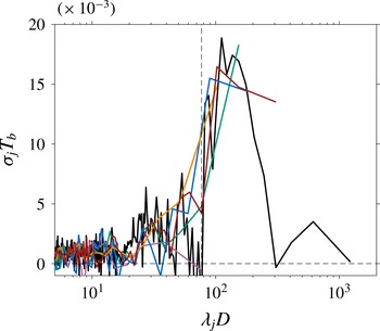
Amplitude growth rate
 $\unicode[STIX]{x1D70E}_{j}$
(as per definition (5.2)) as a function of the wavelength in the first exponential growth regime: — (purple), case H3; — (orange), case H4; — (green), case H6; — (blue), case H7; — (brown), case H12; —, case H48. The vertical dashed line represents the value of the streamwise box length in case H3 which does not feature patterns.

Figure 5 shows the growth rate as a function of the wavelength
 $\unicode[STIX]{x1D706}_{j}\equiv 2\unicode[STIX]{x03C0}/\unicode[STIX]{x1D705}_{j}$
. As is expected, none of the modes are seen to grow at any significant rate in case H3. Moreover, consistent with the evolution of the mean wavelength, the fastest growing mode in cases H4 and H6 is
 $\unicode[STIX]{x1D706}_{1}=L_{x}$
, with a growth rate which is comparable to that of the r.m.s. bed height
 $\unicode[STIX]{x1D70E}_{h}$
(coefficient
 $B$
in (5.1)). The next few modes in these two cases also exhibit a small but noticeable growth rate although their wavelength is smaller than the threshold. This could be attributed to nonlinear effects. A similar trend is observable for cases H7 and H12, except that in these cases, it is not only one harmonic which is growing the fastest. In case H7 both
 $\unicode[STIX]{x1D706}_{1}=L_{x}$
and
 $\unicode[STIX]{x1D706}_{2}=L_{x}/2$
grow at a comparable rate, indicating that both harmonics contribute substantially to the growth of
 $\unicode[STIX]{x1D70E}_{h}$
. On the other hand, in case H12, in addition to the expected fastest growing modes
 $\unicode[STIX]{x1D706}_{3}=L_{x}/3$
and
 $\unicode[STIX]{x1D706}_{2}=L_{x}/2$
, the first harmonic
 $\unicode[STIX]{x1D706}_{1}=L_{x}$
is also seen to contribute to the overall growth. It is not guaranteed that the box length of H48 is large enough to capture all the unstable modes (i.e. the upper threshold of pattern formation). Nevertheless, the fact that
 $\unicode[STIX]{x1D70E}_{j}$
exhibits a clear local maximum is an indication that the box is sufficient to capture the most amplified mode(s), which turn out to be in the range
 $\unicode[STIX]{x1D706}_{8}$
to
 $\unicode[STIX]{x1D706}_{12}$
.
Finally, it is worth mentioning that the computational box sizes are chosen such that a turbulent flow state is sustained. This is confirmed by monitoring the time evolution of the box-averaged turbulent kinetic energy (plots not shown). Note that, in smooth wall channel flows, the minimum spanwise and streamwise box dimensions required in order for turbulence to be self-sustained are
 $L_{z}^{+}\approx 100$
and
 $L_{x}^{+}\approx 350$
, respectively (Jiménez & Moin Reference Jiménez and Moin1991). The minimum box dimensions adopted in our study (corresponding to case H3) are substantially larger, i.e.
 $L_{x}^{+}=L_{z}^{+}\approx 740$
.
5.2 Ripple morphology
An additional important advantage of adopting a relatively ‘small’ computational box length in cases H4, H6 and H7 is that, once the maximum possible wavelength is attained, further ripple dimension growth is effectively hindered. Thus, the accommodated ripple subsequently evolves, steadily maintaining its dimensions and propagation velocity. Similarly, in case H12, within the simulated interval, the ripples evolve steadily, constrained approximately at a mean wavelength
 $\unicode[STIX]{x1D706}_{h}=L_{x}/2$
. Such a numerical manipulation, which experimentally is not possible, allows us to address steady-state bedform characteristics at a particular wavelength. In the following, we analyse the two-dimensional shape and the propagation velocity of the ripples.
It is well know that bedforms of finite amplitude evolve towards an asymmetric shape even in the absence of flow separation (Best Reference Best2005; Colombini & Stocchino Reference Colombini and Stocchino2008; Seminara Reference Seminara2010). For instance, spatio-temporal plots provided by Ouriemi et al. (Reference Ouriemi, Aussillous and Guazzelli2009) show that the evolution of the bedforms towards their asymmetric shape is a phenomenon of both the laminar ‘small dunes’ which exhibit no flow separation in their leeside, as well as the turbulent ‘vortex dunes’ which are characterized by flow separation downstream of their crests. The degree of asymmetry is generally larger in the latter as a result of the flow recirculation. Moreover, the animations of particle motion available online at https://doi.org/10.1017/jfm.2014.284 and the space–time plots depicted in figure 4 of Kidanemariam & Uhlmann (Reference Kidanemariam and Uhlmann2014a ) have qualitatively shown the asymmetric evolution of sediment-bed shape in good agreement with what is observed experimentally.
In order to quantitatively characterize the statistically two-dimensional shape of the bedforms, in the steady ripple evolution interval of cases H4, H6, H7 and H12, we have evaluated the phase-averaged fluid–bed interface which is defined as follows:
 $$\begin{eqnarray}\widetilde{H}_{b}(\tilde{x})=\langle h_{b}(\tilde{x},t)\rangle _{t},\end{eqnarray}$$
where
 $\tilde{x}\equiv x-u_{D}t$
is the
 $x$
-coordinate in a frame of reference which is moving at the mean ripple propagation velocity
 $u_{D}$
(see § 5.3 for the definition of
 $u_{D}$
). Note that, in cases H4, H6 and H7,
 $\widetilde{H}_{b}$
corresponds to the mean profile of a single ripple, while in case H12,
 $\widetilde{H}_{b}$
is an average profile over the two available ripples.
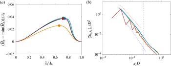
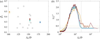
(a) Mean two-dimensional profile of the patterns averaged over the last steady ripple propagation interval, and over the number of ripples when applicable, of each case. The location of the maximum of each profile is shown by the filled symbols. Note that the profiles are plotted not to scale and thus the aspect ratio is visually exaggerated. (b) The corresponding spectra of the sediment-bed-height fluctuation. In both plots: — (orange), case H4; — (green), case H6; — (blue), case H7; — (brown), case H12. Power laws with exponent
 $-3.3$
and
 $-4.3$
are shown by the red and blue dashed lines respectively. The vertical dashed line represents the value of the average fluid height
 $H_{f}\approx 25.27D$
(averaged over all cases).

As shown figure 6(a), it can be seen that in all cases, the ripple profile is clearly asymmetric with an upstream face (upstream of the crest) approximately three times longer in streamwise length and thus milder in bed slope than the downstream face. To within the statistical uncertainty, the bed shape of cases H6, H7 and H12, once scaled by the corresponding mean wavelength, seems to fairly collapse into a single shape, exhibiting small differences. The attained value of the aspect ratio, which is defined as the ratio between the height of the ripple
 $H_{D}=\max (\widetilde{H}_{b})-\min (\widetilde{H}_{b})$
(i.e. the wall-normal distance between the trough and the crest) and the mean wavelength
 $\unicode[STIX]{x1D706}_{h}$
, is approximately 0.037. Moreover, the degree of asymmetry, which can be defined as the ratio between the streamwise distance from the crest to the downstream trough and the mean wavelength, is approximately 0.28. On the other hand, the mean ripple shape of case H4 is seen to exhibit a noticeable smaller value of the aspect ratio (approximately 0.026) and a larger value of the degree of asymmetry (approximately 0.35) than the other cases. This difference is an indication of the ripple shape evolution process. Some experimental studies reported that, during the natural ripple coarsening process, the aspect ratio of the ripple geometry evolves with time and attains a value of approximately
 $1/15$
(
 $0.067$
) once the steady-state shape is attained (Charru et al.
Reference Charru, Andreotti and Claudin2013). On the other hand, Fourrière, Claudin & Andreotti (Reference Fourrière, Claudin and Andreotti2010), based on field measurements, report a steady-state aspect ratio of approximately
 $0.045$
. In our configurations, since the final ‘natural’ steady-state regime is not yet reached, we cannot confidently say that the attained values of the aspect ratios are representative of those values which would naturally be attained. Nevertheless, the fact that the shape of the ripple with mean wavelength
 $\unicode[STIX]{x1D706}_{h}\approx 150D$
and that with
 $\unicode[STIX]{x1D706}_{h}\approx 180D$
do not exhibit substantial differences could be an indication that the ripple shape is not far from its final invariant shape. This aspect requires further investigation.
It is generally believed that the nonlinear interaction between the evolving sediment bed and the driving flow results in the above mentioned asymmetric ripple shape (Charru et al.
Reference Charru, Andreotti and Claudin2013). That is, although the ripples have one well-defined length scale (the mean wavelength
 $\unicode[STIX]{x1D706}_{h}$
defined in (4.6)), a wide spectrum of modes interact nonlinearly to maintain a shape-invariant ripple which propagates downstream. There are several theoretical studies as well as field and experimental measurements which report that the spectra of fully developed bedforms exhibit a
 $-3$
power-law relationship with respect to the large wavenumbers, bounded by a threshold value (Hino Reference Hino1968; Jain & Kennedy Reference Jain and Kennedy1974; Nikora, Sukhodolov & Rowinski Reference Nikora, Sukhodolov and Rowinski1997; Coleman & Nikora Reference Coleman and Nikora2011). To gain further insight, we present in figure 6(b) the spectra
 $\langle S_{h_{b}h_{b}}\rangle _{t}$
of the sediment-bed-height fluctuation averaged over the steady ripple evolution interval of the above-mentioned cases. It can be seen that, for the dominant modes (with
 $\unicode[STIX]{x1D706}_{j}\gtrsim H_{f}$
),
 $\langle S_{h_{b}h_{b}}\rangle _{t}$
of all the cases (only for the even modes of case H12) features a power-law variation as a function of
 $\unicode[STIX]{x1D705}_{j}$
. The value of the scaling exponent in cases H6, H7 and for the even modes in H12 is observed to be approximately
 $-3.3$
whereas that of case H4 is approximately
 $-4.3$
. The fact that case H4 has a larger value of the exponent than that of the other cases is again an indication of the evolution process. That is, the influence on the mean ripple shape of the modes with a smaller wavelength than the dominant one is relatively smaller compared to the other cases. Moreover, the fact that we have not attained a naturally developed mature ripple state could be a reason why the attained exponents are slightly larger than the
 $-3$
value reported in the literature. The reason for the odd–even separation of the spectra in case H12 could be explained by the fact that the domain length accommodates two ripples and thus modes with wavelength
 $L_{x}/(2i)$
mainly contribute to the attained shape.
5.3 Ripple migration velocity
The migration velocity of bedforms is an important quantity of interest in the study of morphodynamics. For instance, the rate at which bedforms propagate is closely related to the rate of sediment transport (Coleman & Melville Reference Coleman and Melville1994; Nikora et al.
Reference Nikora, Sukhodolov and Rowinski1997; Betat et al.
Reference Betat, Kruelle, Frette and Rehberg2002; Coleman et al.
Reference Coleman, Fedele and Garca2003; Coleman & Nikora Reference Coleman and Nikora2009b
; Ouriemi et al.
Reference Ouriemi, Aussillous and Guazzelli2009; Seminara Reference Seminara2010). From the sediment mass-conservation equation (Exner equation), it can be easily shown that, for a statistically shape-invariant two-dimensional ripple with height
 $H_{D}$
and which migrates downstream at a constant velocity
 $u_{D}$
,
 $$\begin{eqnarray}\langle q_{p}\rangle -\langle q_{p,min}\rangle \approx \unicode[STIX]{x1D6FD}\unicode[STIX]{x1D6F7}_{b}u_{D}H_{D},\end{eqnarray}$$
where
 $\langle q_{p}\rangle$
is the mean particle flow rate, which is assumed to be constant, while
 $\langle q_{p,min}\rangle$
is the corresponding minimum value at the trough of the ripple,
 $\unicode[STIX]{x1D6F7}_{b}$
is the mean solid volume fraction of the sediment bed and
 $\unicode[STIX]{x1D6FD}$
is a ripple shape parameter. From the approximation (5.4), it is evident that the ripple migration velocity is inversely proportional to the ripple height (and thus the ripple mean wavelength) whereas it is directly proportional to the mean particle flow rate (Charru et al.
Reference Charru, Andreotti and Claudin2013). In the following, based on the DNS data, we evaluate the mean ripple migration velocity and assess its relation to the mean particle flow rate.
In the aforementioned steady evolution interval, an average migration velocity of the patterns
 $u_{D}$
can be determined from the shift of the maximum of space–time correlation function of the fluid–bed interface fluctuation
 $h_{b}^{\prime }$
(Nikora et al.
Reference Nikora, Sukhodolov and Rowinski1997; Coleman & Nikora Reference Coleman and Nikora2011). First, the space–time correlation function is defined as follows:
 $$\begin{eqnarray}R_{ht}(\unicode[STIX]{x1D6FF}x,\unicode[STIX]{x1D6FF}t)=\langle h_{b}^{\prime }(x,t_{1})\cdot h_{b}^{\prime }(x+\unicode[STIX]{x1D6FF}x,t_{1}+\unicode[STIX]{x1D6FF}t)\rangle _{x}\quad \forall \unicode[STIX]{x1D6FF}t\in \left[0,t_{2}-t_{1}\right],\end{eqnarray}$$
where
 $t_{1}$
and
 $t_{2}$
are the start and end times of the considered interval. The streamwise location
 $x_{max}$
of the maximum of
 $R_{ht}$
, which is given by
 $$\begin{eqnarray}r_{x}^{m}(\unicode[STIX]{x1D6FF}t)=x_{max}(\unicode[STIX]{x1D6FF}t)\;|\;\forall \,\unicode[STIX]{x1D6FF}x\in [-L_{x}/2,\;L_{x}/2]:R_{ht}(\unicode[STIX]{x1D6FF}x,\unicode[STIX]{x1D6FF}t)\leqslant R_{ht}(x_{max},\unicode[STIX]{x1D6FF}t),\end{eqnarray}$$
varies approximately linearly with respect to
 $\unicode[STIX]{x1D6FF}t$
, and thus the slope of the line which is fitted to the data
 $r_{x}^{m}$
versus
 $\unicode[STIX]{x1D6FF}t$
gives an accurate estimate of
 $u_{D}$
.
(a) Average propagation speed of the patterns, normalized in wall units, as a function of the mean wavelength (computed in the final steady ripple evolution interval as shown in table 2): ▴ (orange), case H4; ◂ (green), case H6; ▸ (blue), case H7; ● (brown), case H12. The corresponding cross-marks (
 $\times$
) represent the mean ripple migration velocity estimated by relation (5.4). The data points in the turbulent channel flow experiment of Cardona Florez & Franklin (Reference Cardona Florez and Franklin2016) for their particles with diameter
 $D=550~\unicode[STIX]{x03BC}\text{m}$
are shown by the open symbols ○ (initial phase of ripple evolution) and ▫ (final phase of the evolution). (b) Mean propagation speed of individual Fourier modes in the final steady ripple evolution interval: — (orange), case H4; — (green), case H6; — (blue), case H7; — (brown), case H12. The corresponding mean ripple migration velocity is plotted by the horizontal dashed lines. The vertical dashed line represents the value of the average fluid height
 $H_{f}\approx 25.27D$
(averaged over all cases). In both plots, ensemble averaging is performed for cases H4 and H12 over the available number of runs.

Figure 7(a) shows the migration velocity, normalized by
 $u_{\unicode[STIX]{x1D70F}}$
, as a function of the mean wavelength for cases H4, H6, H7 and H12. The variation of
 $u_{D}$
exhibits an inverse relationship with the ripple wavelength, varying from a value
 $u_{D}^{+}\approx 0.49$
for case H4 down to a value
 $u_{D}^{+}\approx 0.3$
for case H7. It should be noted, however that, as will be shown in § 5.5, as a consequence of an increase of the mean bottom shear stress, the value of the mean particle flow rate increases with increasing mean wavelength. Thus the observed trend of the ripple migration velocity is a net result of an increase of particle flow rate as well as an increase of ripple dimensions. In the following, we assess the mass-conservation-based relationship between the mean particle flow rate and the ripple migration velocity, by reverse-computing the latter from relation (5.4). To this end, a mean particle flow rate
 $\langle q_{p}\rangle$
is computed over the steady ripple migration interval (cf. § 5.5). The average minimum particle flow rate at the ripple troughs
 $\langle q_{p,min}\rangle$
was computed as well. It turns out that the value
 $\langle q_{p,min}\rangle$
is negligibly small in cases H6, H7 and H12, whereas in case H4 it attains a value of
 $\langle q_{p,min}\rangle \approx 0.2\langle q_{p}\rangle$
. Furthermore, the ripple shape parameter
 $\unicode[STIX]{x1D6FD}$
is defined as the ratio between the two-dimensional area of the ripple to that of a bounding rectangle of dimensions
 $H_{D}$
and
 $\unicode[STIX]{x1D706}_{h}$
, defined as
 $$\begin{eqnarray}\unicode[STIX]{x1D6FD}=\frac{1}{H_{D}\unicode[STIX]{x1D706}_{h}}\int _{0}^{\unicode[STIX]{x1D706}_{h}}(\widetilde{H}_{b}(x)-\min (\widetilde{H}_{b}))\,\text{d}x.\end{eqnarray}$$
In most of the engineering-purpose bedload transport rate estimators, the value of
 $\unicode[STIX]{x1D6FD}$
is typically taken to be
 $0.5$
, assuming that the shape of the ripple is triangular, while some adopt values up to
 $\unicode[STIX]{x1D6FD}=0.6$
based on field and experimental measurements (see e.g. Gaeuman & Jacobson (Reference Gaeuman and Jacobson2007) and references therein). For the mean ripple geometries encountered in the present study, a value of
 $\unicode[STIX]{x1D6FD}$
in the range between
 $0.5$
and
 $0.52$
is recovered after evaluating (5.7) for all the cases. Subsequently, the mean ripple migration velocity is estimated based on relation (5.4) and the result is presented in figure 7(a). It can be seen that the estimation yields values which are in good agreement with the actual computed ripple migration velocity values.
Additionally, figure 7(a) shows recent experimental measurements of ripple migration velocity in a closed-conduit set-up (Cardona Florez & Franklin Reference Cardona Florez and Franklin2016). The experimental data shown correspond to particles with diameter
 $D=550~\unicode[STIX]{x03BC}\text{m}$
(
 $Re_{b}\approx 7600{-}8900$
,
 $\unicode[STIX]{x1D70C}_{p}/\unicode[STIX]{x1D70C}_{f}=2.5$
,
 $H_{f}/D\approx 39$
,
 $\unicode[STIX]{x1D703}\approx 0.056{-}0.075$
,
 $D^{+}\approx 12{-}14$
,
 $Ga\approx 50$
) which is not far from our parameter point. Although the experimental data exhibit relatively large scatter, it can be seen that the trend of the DNS data falls within the experimental data cloud.
Finally, let us turn to the celerity of the individual Fourier modes of the bedforms. The phase angle spectrum
 $\unicode[STIX]{x1D711}_{j}$
of the sediment-bed-height fluctuation is defined as
 $$\begin{eqnarray}\unicode[STIX]{x1D711}_{j}(t)=\text{atan2}(\text{Re}({\hat{h}}_{bj}(t)),\text{Im}({\hat{h}}_{bj}(t)))\quad \forall j=0,\ldots ,N_{x}/2,\end{eqnarray}$$
where ‘atan2’ is the four-quadrant inverse tangent. The instantaneous value of the phase speed
 $c_{j}$
is derived from (5.8) as:
 $$\begin{eqnarray}c_{j}(t)=-\frac{1}{\unicode[STIX]{x1D705}_{j}}\frac{\text{d}\unicode[STIX]{x1D711}_{j}}{\text{d}t}(t).\end{eqnarray}$$
In the steady ripple propagation interval of cases H4, H6, H7 and H12, we have evaluated an average mode-wise phase speed
 $\langle c_{j}\rangle$
which is presented in figure 7(b) as a function of the wavelength
 $\unicode[STIX]{x1D706}_{j}$
. In all the considered cases, the celerity data feature two distinct types of modes: dispersive and non-dispersive. All harmonics with a wavenumber value smaller than a threshold are observed to be non-dispersive, propagating at the corresponding mean ripple migration velocity. To within the statistical uncertainty of the data, the threshold value is the same in all cases and turns out to be
 $\unicode[STIX]{x1D706}_{j}\approx H_{f}$
. Note that the non-dispersive modes are those dominant ones which exhibit a power-law relationship in figure 6. On the other hand, the remaining harmonics with a wavelength smaller than the threshold are observed to be dispersive, exhibiting approximately the same variation of the phase speed as a function of the wavelength in all cases. The trend is seen to be well defined when scaled by the friction velocity, increasing from its value at the threshold location and attaining values of
 $\langle c_{j}\rangle ^{+}\approx 2$
at wavelengths of approximately
 $\unicode[STIX]{x1D706}_{j}\approx 10D$
. At first glance, the observations of dispersive modes seems incompatible with the fact that the ripples are migrating at a constant velocity maintaining their two-dimensional shape. Looking at figure 6, however, the contribution of the fast-moving modes to the mean ripple shape (and mean migration velocity) is orders of magnitude smaller than that of the most dominant one, thus negligible. These modes are footprints of the particle erosion/deposition cycle which takes place on the top of the ripples. Based on field measurements, Nikora et al. (Reference Nikora, Sukhodolov and Rowinski1997) similarly report that fully developed ripples are composed of non-dispersive modes with wavelength
 $\unicode[STIX]{x1D706}\gg H_{f}$
, as well as dispersive modes with
 $\unicode[STIX]{x1D706}\ll H_{f}$
, corroborating our findings.
5.4 Mean shear stress at the fluid–bed interface
For a given imposed flow rate, an increase of the mean interface shear stress with increasing ripple dimensions is expected since the ripples are effectively roughness elements of the sediment bed (cf. Jiménez Reference Jiménez2004, for instance). This in turn is expected to influence the mean rate of particle transport in a given channel, since it is directly proportional to the mean shear stress. The inter-dependency among the evolving ripple, the mean interface shear stress and the mean particle flow rate can be assessed by evaluating these quantities on the steady interval of each case (cf. table 2).
Let us recall that the driving volume force exerted by the imposed mean pressure gradient
 $\langle \text{d}p/\text{d}x\rangle$
in a particle-laden channel flow is balanced by the sum of resisting force of the fluid shear stress and stress contribution from the fluid–particle interaction. In the context of the immersed boundary method, the volume force, which imposes the no-slip condition at the fluid–particle interface, corresponds to the stress imposed on the system as a result of the fluid–solid interaction (see e.g. Uhlmann Reference Uhlmann2008; Kidanemariam et al.
Reference Kidanemariam, Chan-Braun, Doychev and Uhlmann2013). When the momentum equation is averaged over the entire domain comprising the fluid and particles, the streamwise momentum balance reduces to
 $$\begin{eqnarray}-\left\langle \frac{\text{d}p}{\text{d}x}\right\rangle (L_{y}-y)=\underbrace{\unicode[STIX]{x1D70C}_{f}\unicode[STIX]{x1D708}\unicode[STIX]{x2202}_{y}\langle u\rangle -\unicode[STIX]{x1D70C}_{f}\langle u^{\prime }v^{\prime }\rangle +\int _{y}^{L_{y}}\langle f_{x}\rangle \,\text{d}y}_{\langle \unicode[STIX]{x1D70F}_{tot}\rangle },\end{eqnarray}$$
where the last term in the right-hand side represents the fluid–solid interaction,
 $\langle u\rangle$
is the mean composite velocity, and
 $\langle u^{\prime }v^{\prime }\rangle$
is the covariance with respect to
 $\langle u\rangle$
. When (5.10) is applied to a statistically one-dimensional channel flow configuration (for instance case H3),
 $\langle u^{\prime }v^{\prime }\rangle$
represents the momentum flux due to turbulent fluctuations. On the other hand, the mean flow in those ripple-featuring cases is two-dimensional and
 $\langle u^{\prime }v^{\prime }\rangle$
represents not only the turbulent fluctuations, but also contribution from the deviation of the mean flow streamlines from the streamwise direction (see e.g. Yalin Reference Yalin1977; Nikora et al.
Reference Nikora, McEwan, McLean, Coleman, Pokrajac and Walters2007). A detailed analysis of the flow field over bedforms is not part of the current study and will appear in a followup paper. Here, in order to define a mean interface shear stress, evaluating (5.10) suffices. In the steady ripple propagation interval of the current configuration (cf. table 2),
 $\langle \unicode[STIX]{x1D70F}_{tot}\rangle$
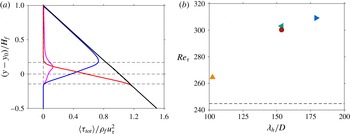
should vary linearly as a function of wall-normal distance. This is confirmed in figure 8(a), which shows the wall-normal variation of the different contributions to the total shear stress for case H7. The remaining cases exhibit similar trends (plots not shown). The figure highlights that, in the region above the highest crest of the ripples, the driving force is dominantly balanced by the fluid stress term while in the domain below the lowest trough of the ripples, the particle-related forcing entirely balances the pressure gradient forcing. The mean interface shear stress (
 $\unicode[STIX]{x1D70C}_{f}u_{\unicode[STIX]{x1D70F}}^{2}$
) is thus defined as the value of
 $\langle \unicode[STIX]{x1D70F}_{tot}\rangle$
at the location of the mean fluid–bed interface
 $y_{0}=H_{b}$
. It should be noted that, in the ripple-featuring cases, due to the roughness introduced as a result of the evolving bedforms, a horizontal fluid–bed interface does not exist. Nevertheless, a virtual wall could be defined to be located at a wall-normal location
 $y_{0}=H_{b}$
.
(a) Wall-normal profiles of the different contributions to the total shear stress of case H7 (computed in the final steady ripple evolution interval as shown in table 2): — (magenta),
 $\unicode[STIX]{x1D70C}_{f}\unicode[STIX]{x1D708}\unicode[STIX]{x2202}_{y}\langle u\rangle$
; — (blue),
 $-\unicode[STIX]{x1D70C}_{f}\langle u^{\prime }v^{\prime }\rangle$
; — (red),
 $\int _{y}^{L_{y}}\langle f_{x}\rangle \,\text{d}y$
; —,
 $\langle \unicode[STIX]{x1D70F}_{tot}\rangle$
. The horizontal dashed lines represent the wall-normal location of mean fluid–bed interface as well as its all-time maximum and minimum extents over the considered observation interval. (b) Friction velocity based Reynolds number as a function of the mean wavelength
 $\unicode[STIX]{x1D706}_{h}$
in the corresponding steady ripple evolution interval: ▴ (orange), case H4; ◂ (green), case H6; ▸ (blue), case H7; ● (brown), case H12. The horizontal dashed line corresponds to the value of
 $Re_{\unicode[STIX]{x1D70F}}$
in the featureless case H3.

Figure 8(b) shows the mean interface shear stress (expressed in terms of the friction velocity based Reynolds number) as a function of the mean ripple wavelength for the different cases (computed in the final steady ripple evolution interval as shown in table 2). It can be seen that the value of the friction Reynolds number in the featureless case H3 is
 $Re_{\unicode[STIX]{x1D70F}}\approx 245$
. This value is larger than the value of
 $Re_{\unicode[STIX]{x1D70F}}$
in a rough-wall channel flow at a comparable bulk Reynolds number and at roughly the same particle Reynolds number (cf. Chan-Braun, García-Villalba & Uhlmann Reference Chan-Braun, García-Villalba and Uhlmann2011). The main difference between the latter case and the present case H3 is the particle arrangement and particle mobility, i.e. the erosion, entrainment and re-deposition cycle. Furthermore, when comparing the friction Reynolds number of cases H4, H6, H7 and H12, it can be observed that there is a monotonic increase with increasing wavelength, attaining values
 $Re_{\unicode[STIX]{x1D70F}}\approx 265$
for
 $\unicode[STIX]{x1D706}_{h}\approx 102D$
,
 $Re_{\unicode[STIX]{x1D70F}}\approx 300$
for
 $\unicode[STIX]{x1D706}_{h}\approx 154D$
and
 $Re_{\unicode[STIX]{x1D70F}}\approx 310$
for
 $\unicode[STIX]{x1D706}_{h}\approx 180D$
. Recalling the fact that the imposed fluid flow rate and the mean fluid height are essentially the same in all cases, the increase in the shear stress among the ripple-featuring cases is entirely a consequence of the increase of the amplitude of the evolving sediment patterns (i.e. the macroscopic roughness height).
5.5 Mean particle flow rate
The instantaneous volumetric flow rate of the particle phase (per unit span),
 $q_{p}$
, is given by the sum (over all particles) of the streamwise particle velocity times the particle volume, divided by the product of the streamwise and spanwise extent of the domain (Kidanemariam & Uhlmann Reference Kidanemariam and Uhlmann2014
b
), viz
 $$\begin{eqnarray}q_{p}(t)=\frac{\unicode[STIX]{x03C0}D^{3}}{6L_{x}L_{z}}\mathop{\sum }_{l=1}^{N_{p}}u_{p}^{(l)}(t),\end{eqnarray}$$
where
 $u_{p}^{(l)}(t)$
is the streamwise component of the instantaneous velocity of the
 $l$
th mobile particle at time
 $t$
. Averaging
 $q_{p}$
over a given stationary interval results in the mean particle flow rate
 $\langle q_{p}\rangle$
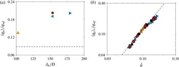
in that interval. We remark that, for the parameter point considered in the present study, particles are dominantly transported as ‘bedload’ material. Only a very small fraction of the mobile particles is suspended and entrained by the mean flow. Thus, the particle flow rate defined in (5.11) represents overwhelmingly the former mode of transport. In figure 9(a), as a consequence of the increased mean bottom friction, the mean particle flow rate is observed to increase with increasing ripple dimensions.
Of particular relevance to engineering applications is to express the particle flow rate as a function of the Shields number and to pursue scaling laws which relate the two quantities. In order to analyse the particle flow rate obtained in the present work in light of such scaling laws, the non-dimensional particle flow rate (normalized by the inertial scale
 $q_{ref}=U_{g}D$
) is shown as a function of the excess Shields number
 $\tilde{\unicode[STIX]{x1D703}}=\unicode[STIX]{x1D703}-\unicode[STIX]{x1D703}_{c}$
in figure 9(b), using the value
 $\unicode[STIX]{x1D703}_{c}=0.034$
according to the empirical law proposed by Soulsby & Whitehouse (Reference Soulsby and Whitehouse1997). Since all the ripple-featuring cases have started from an initially flat sediment bed, the values of both the shear stress and the particle flow rate in these cases increase with time from their initial values to their final values at the end of the simulation interval. In order to capture this time evolution, the entire observation interval of each case is decomposed into smaller intervals of approximately 25 bulk time units. A mean particle flow rate and bottom shear stress is then computed for each interval, substantially increasing the data samples in the figure. The duration of the time intervals is chosen to be much smaller than the time scales of the ripple evolution. Figure 9(b) also shows the empirical power law of Wong & Parker (Reference Wong and Parker2006), which in turn is a modified version of the Meyer-Peter & Müller (Reference Meyer-Peter and Müller1948) formula for turbulent flows,
 $$\begin{eqnarray}\langle q_{p}\rangle /q_{ref}=A\tilde{\unicode[STIX]{x1D703}}^{\unicode[STIX]{x1D6FC}},\end{eqnarray}$$
where
 $A=4.93$
and
 $\unicode[STIX]{x1D6FC}=1.6$
. Note that Wong & Parker’s formula is valid for a macroscopically flat sediment bed. As is observed in the figure, the DNS data points, which represent both plane sediment beds as well as pattern-featuring beds, are in very good agreement with the scaling law (5.12). Although the evolution of the ripples does increase the net particle transport rate, the net bottom shear stress simultaneously increases. As a net result, the formation of patterns does not strongly affect the particle transport scaling as a function of the excess shear stress (in the considered observation interval).
(a) Volumetric particle flow rate
 $\langle q_{p}\rangle$
as a function of the mean wavelength
 $\unicode[STIX]{x1D706}_{h}$
(computed in the final steady ripple evolution interval as shown in table 2): ▴ (orange), case H4; ◂ (green), case H6; ▸ (blue), case H7; ● (brown), case H12. The horizontal dashed line corresponds to the value of
 $\langle q_{p}\rangle$
in the featureless case H3. (b) Particle flow rate
 $\langle q_{p}\rangle _{i}$
as a function of the excess Shields number
 $\tilde{\unicode[STIX]{x1D703}}=\unicode[STIX]{x1D703}-\unicode[STIX]{x1D703}_{c}$
. The entire observation interval of each case is decomposed into smaller intervals of approximately 25 bulk time units: ▴ (purple), case H3; ▴ (orange), case H4; ◂ (green), case H6; ▸ (blue), case H7; ● (brown), case H12; ▪, case H48. A mean particle flow rate and bottom shear stress is then computed for each interval (thus the notations
 $\langle q_{p}\rangle _{i}$
and
 $\unicode[STIX]{x1D703}_{i}$
). Note that values for every fifth interval are plotted for clarity. The value
 $\unicode[STIX]{x1D703}_{c}=0.034$
is used in order to compute
 $\tilde{\unicode[STIX]{x1D703}}$
for the current DNS data, according to the empirical law proposed by Soulsby & Whitehouse (Reference Soulsby and Whitehouse1997). The dashed line is the Wong & Parker (Reference Wong and Parker2006) version of the Meyer-Peter & Müller (Reference Meyer-Peter and Müller1948) formula for turbulent flow which reads:
 $\langle q_{p}\rangle /q_{ref}=4.93\,\tilde{\unicode[STIX]{x1D703}}^{1.6}$
.

6 Conclusion
We have performed several direct numerical simulations of the development of bedforms over an erodible sediment bed in an open channel flow configuration. All the simulations were carried out at a parameter point which is identical to our previous study (Kidanemariam & Uhlmann Reference Kidanemariam and Uhlmann2014a
). The simulations differ only in the adopted streamwise length of the computational domain, which was systematically varied in order to address important aspects of pattern formation. Ensemble averaging was performed for two select cases in order to account for the statistical variability during the transients. By reducing the domain size, we were able to find the lower bound of the unstable pattern wavelength, below which pattern formation is effectively hindered and the sediment bed remains stable. The strategy is similar to the minimal flow unit of Jiménez & Moin (Reference Jiménez and Moin1991). For the considered parameter point, it turns out that a computational box with a streamwise dimension
 $L_{x}\lesssim 75D$
, where
 $D$
is the particle diameter, was not sufficient to accommodate any of the unstable modes, and no sediment features were observed. On the contrary, a box with
 $L_{x}\gtrsim 100D$
accommodated at least one unstable mode. This observation indicates that the cutoff length lies in the range
 $75$
–
 $100D$
(
 $3$
–
 $4$
times the clear fluid height).
Furthermore, the influence of the computational domain size on the selection and evolution of the initial wavelength was assessed by performing one large-scale simulation with streamwise box length
 $L_{x}\approx 1200D$
(
 $48H_{f}$
) and with approximately
 $1.1$
million resolved particles representing the mobile bed. This allowed the determination of the most amplified wavelength(s) to be determined with sufficient accuracy. It turns out that, during the initial bed instability, the box was able to accommodate a number of ripple units with a mean wavelength
 $\unicode[STIX]{x1D706}_{c}\approx 100$
–
 $110D$
(values which correspond to the wavelength of the eleventh and twelfth resolved harmonics in that case). Based on the comparison of the selected mean wavelength among the different simulated cases, it can be concluded that a computational domain length which is few integer multiples of
 $\unicode[STIX]{x1D706}_{c}$
, due to the sparsity of the resolved discrete harmonics, severely constrains the natural ripple initiation and evolution mechanisms. The domain length adopted by Kidanemariam & Uhlmann (Reference Kidanemariam and Uhlmann2014a
), which accommodated approximately three initial ripple units, was observed to be marginally sufficient in determining the initial wavelength, while too small to capture the subsequent evolution.
Based on the analysis of the r.m.s. sediment-bed-height fluctuation, two regimes of pattern evolution were identified. An initial short-lived exponential growth regime (with a duration of approximately 200 bulk time units) and a subsequent nonlinear regime. The evolution of the r.m.s. bed fluctuation is observed to be independent of the chosen domain size in the initial exponential regime, while it exhibited a strong influence of the domain size in its later stages. The exponential growth of the sediment-bed fluctuation is further scrutinized by analysing the dispersion relation of the unstable modes, i.e. the growth rate of the individual Fourier harmonics which make up the resolved spectrum. The latter, which is difficult to access experimentally, is an important quantity of interest when it comes to assessing the validity of the various theoretical models (Charru et al.
Reference Charru, Andreotti and Claudin2013). It turns out that, to within the statistical uncertainty of our data, the modes which are initially growing at a substantial rate are those with a wavelength approximately in the range
 $\unicode[STIX]{x1D706}_{j}=100$
–
 $200D$
and are roughly bounded by an upper limit of
 $\unicode[STIX]{x1D706}_{j}=300D$
.
Furthermore, the conditions of our simulations have allowed us to impose a steady ripple evolution at a desired wavelength. That is, in the simulation cases in which
 $L_{x}/\unicode[STIX]{x1D706}_{c}=O(1)$
, after the initial exponential growth interval, the system chooses the maximum possible mean wavelength
 $\unicode[STIX]{x1D706}_{h}=L_{x}$
relatively quickly. Subsequently, the accommodated ripple evolves steadily, maintaining a statistically time-invariant shape and migration velocity. This allows one to address aspects such as characterization of the two-dimensional asymmetrical ripple shape, ripple migration velocity and the relation of the latter to the mean particle flow rate. It was found that the spectrum of the sediment-bed elevation follows a power-law decay over the first few dominant modes, with an exponent which exhibited a slight dependence on the evolution of the mean wavelength. The value of the exponent obtained from the DNS data is not too far from the value of ‘
 $-3$
’ for fully developed bedforms as proposed in the literature (Hino Reference Hino1968; Nikora et al.
Reference Nikora, Sukhodolov and Rowinski1997). Additionally, the relation of the ripple migration velocity to the mean particle flow rate was addressed by computing the former from the shift of the space–time correlation function of the sediment-bed height as well as from the sediment mass balance (integration the Exner equation). Both approaches gave comparable results, highlighting the fact that bedforms migrate as a result of erosion of sediment grains from their upstream face and deposition at their downstream fronts.
The volumetric particle flow rate of all the simulated cases is found to be reasonably well predicted by the empirical power law of Wong & Parker (Reference Wong and Parker2006). It should be noted that the evolution of the patterns has indeed increased the net particle transport rate, but at the same time, it has increased the net interface shear stress. Therefore, it can be concluded that the scaling law proposed by these authors still holds in the presence of ripples with an amplitude of the order of a few particle diameters. Whether this statement continues to be true at larger pattern amplitudes needs to be re-assessed by further studies.
Another aspect of the present problem which requires further attention is the influence of the evolving sedimentary patterns upon the turbulent flow. One particularly important question in this context concerns the shear stress distribution at the fluid/sediment-bed interface. The present numerical data set is well-suited for evaluating this quantity as well as other details of the flow field and the particle motion (such as the local, instantaneous relation between the particle flux and the shear stress). This aspect of the problem will be addressed in a future contribution.
Acknowledgements
This work was supported by the German Research Foundation (DFG) through grant UH242/2-1. Part of the simulations have been carried out on SuperMUC at the Leibniz Supercomputing Center (LRZ) of the Bavarian Academy of Science and Humanities. The simulations were also partly performed on the computational resource ForHLR I/II of the Steinbuch Centre for Computing (SCC) funded by the Ministry of Science, Research and the Arts Baden-Württemberg and DFG. The computer resources, technical expertise and assistance provided by the staff at these computer centres are thankfully acknowledged.
Appendix. A note on a programming error in the simulations of Kidanemariam & Uhlmann (Reference Kidanemariam and Uhlmann2014a )
During the preparation of the present manuscript, we have discovered a minor programming error in a subroutine of our simulation code which computes the inter-particle collision forces/torques. This bug was active during the simulations of our previous contribution (Kidanemariam & Uhlmann Reference Kidanemariam and Uhlmann2014a ). All the DNS data in the present work are generated after correcting the aforementioned error. In the following, we assess the influence of the bug by comparing the dune-related quantities extracted from the current data with those reported in Kidanemariam & Uhlmann (Reference Kidanemariam and Uhlmann2014a ).
Time evolution of (a) the r.m.s. sediment-bed-height fluctuation and (b) the mean wavelength
 $\unicode[STIX]{x1D706}_{h}$
. Solid lines correspond to the different realizations of case H12 while the dashed line represents the data corresponding to case ‘T01’ in figure 6 of Kidanemariam & Uhlmann (Reference Kidanemariam and Uhlmann2014a
).

Figure 10 shows the time evolution of the ripple amplitude and mean wavelength of the three different simulations of case H12 (which differ from one another only in the slightly different initial conditions). Additionally, the figure shows the corresponding data from our previous contribution (case ‘T01’ in figure 6 of Kidanemariam & Uhlmann Reference Kidanemariam and Uhlmann2014a ). It can be seen that the difference between the data with and without the bug is within the scatter due to the three independent realizations of case H12. We have further scrutinized the influence of the bug by comparing other less-sensitive quantities such as the particle flow rate and the mean fluid and particle velocities. The results of these quantities are practically not affected by the bug. Thus it can be concluded that the impact of the programming error on the results and conclusions made in Kidanemariam & Uhlmann (Reference Kidanemariam and Uhlmann2014a ) is insignificant.