II. SIMULATION MODEL AND METHOD

As mentioned, we use MD to determine the evolution of the interaction of particles over time by numerically solving Newton's second law. Particles can be atoms, ions, molecules, or polymer chain segments. A set of interaction potentials is used to model the response of pairwise interactions and solved for the entire system, namely,

(1)$$\!\!{m_i}({d^2}/d{t^2}){{\bf{r}}_i}(t) = - {\rm{ }}\nabla U({{\bf{r}}_i}),{\rm{ }}i{\rm{ }} = {\rm{ }}1,{\rm{ }}2,{\rm{ }}3, {\tf="OT3c2d9f11"\char"26}, \ldots ,{\rm{ }}N\quad ,$$

where U(r_i) is the total potential energy between particles i with mass m _i and position r_i at time t. In our case, we have used a computer model of HDPE using the statistical segment approach espoused by Flory,^{Reference Brostow, Donahue, Karashin and Simoes26} with each segment representing roughly two hundred C₂H₄ monomeric units. This is usually called a course-grain^{Reference Luo and Sommer35} model and is used to increase the time and length scales accessible within reasonable computational resources.^{Reference Baschnagel, Binder, Doruker, Gusev, Hahn, Kremer, Mattice, Muller-Plathe, Murat, Paul, Santos, Suter and Tries36} The interaction potentials are based on Mie (often called Lennard Jones) potentials and have been described in more detail in previous papers.^{Reference Brostow and Simoes24,Reference Hilbig, Brostow and Simoes25} In short, the segments have an optimal distance from each other; there is a steeply increasing repulsive force when segments move close to one another and a growing weaker attractive force when they move away from one another. As described in detail in an earlier paper,^{Reference Brostow, Hinze and Simoes37} material generation begins by placing segments on a triangular lattice in a 3D space. Each position then represents a chain with a length of one segment. We form a bond between the two ends of neighboring chains that are the closest together. Since in the beginning all the segments are equidistant, a random number generator is used to determine which segments are bonded. This procedure is continued until no more chains of length two can be created. We then form chains of longer lengths until there are no more neighboring segments at the ends of chains that can be bonded. Thus, the result is a set of randomly coiled nonintersecting chains, with segments on triangular lattice positions, and some vacancies.

Before the indentation process, the material is allowed to equilibrate with no external forces acting. Essentially, the segments are left to interact with each other based on the intersegment and intrasegment interaction potentials. The intrapotential distance is 1.6 times the distance of the interpotential distance. We allow the material to equilibrate for 50 simulation steps. Each simulation step represents 2000 time steps, or 10 ns, meaning that the equilibration equals 0.5 μs. After each time step, segment positions are recalculated. Before equilibration, the segment positions are based on the triangular lattice, where the initial chains are formed, but since intra- and intersegmental equilibrium distances are somewhat different, the lattice positions do not provide a minimum energy configuration. Naturally, the segments are not uniformly spaced after equilibration. Thus, the equilibrium process is necessary so that the material is in a stable state before we add external forces. We perform this equilibration until the segment positions change no more than 1%, a value we have previously used to define full recovery^{Reference Brostow, Hinze and Simoes37} after each simulation step. The model and method used here have been explained earlier.^{Reference Hilbig, Brostow and Simoes25,37−39}

During simulation, an indenter is applied to the center of the top surface of the material. For simplicity, we use a “good” indenter: it does not have any reactions with HDPE. It is simply modeled as an external force applied onto the material. The indentation force is aligned perpendicularly to the surface for a user-defined number of simulation steps. We vary the size of the indenter by the number of segments that exhibit the external force, and the force is divided evenly among all of the segments. A round shape is assumed for the indenter (what defines which segments are selected for applying the force).

After the indentation process has been completed, the indenter is removed. The recovery after indentation is an important process as can be seen from experiments on viscoelastic materials.^{Reference Brostow, Deborde, Jaklewicz and Olszynski40–Reference Brostow, Chonkaew, Mirshams and Srivastava43}

A bounding box model is used for these simulations; to not let the material flatten during simulation, we do not let the outside segments move past the box boundaries. By using this method, our materials have a constant volume, as opposed to other methods of bounding commonly used in small-scale MD simulation studies. Our bounding box method has been explained in more detail in previous work.^{Reference Brostow and Simoes24}

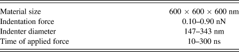
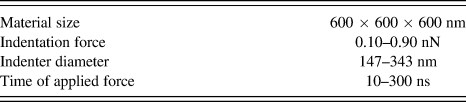
The range of force, indenter size, and time during which the external force is applied is summarized in Table I. The external forces should not cause the indenter to penetrate the material close to the bottom layer as this would produce faulty data. Thus, forces are varied from 0.10 to 0.90 nN. The indenter size ranges from a diameter of three statistical segments, 147 nm, to seven segments, 343 nm. The time during which the external force is applied ranges from 10 to 300 ns.

TABLE I.

Summary of simulation parameters.

The penetration depth is considered as the difference between the average depth of all the segments subjected to the external force and the average of all of the segments on the top row of the material, all measurements being taken from the center of the segments. The max penetration depth R _p is taken as the maximum average depth of the segments subjected to the external force. The recovery depth R _h is taken as the average depth of all the segments subjected to the force after sufficiently long time. In the present study, R _h was determined at 60 simulation steps after the indenter leaves the material. The recovery percentage, ϕ, is obtained from the two previously named parameters as:

(2)$$\varphi = [({R_{\rm{p}}} - {R_{\rm{h}}})/{R_{\rm{p}}}{\rm{ }}] \times 100\quad .$$

III. SELECTED RESULTS

Three simulation parameters are important: the applied external force, the indenter diameter, and the amount of time that the indenter is allowed to penetrate the material. We vary these parameters one at a time.

All the results shown are the average of three unique materials created with the exact same material creation parameters; due to the random nature of the chain formation mechanism, this will result in different amorphous chain spatial arrangements. The random nature of the chain configurations was also studied: thirteen materials, each of same size, were found to have on average 109.9 chains with a standard deviation of 5.2 chains. Figure 1 shows two materials with different chain structures, with each chain represented in a different color.

FIG. 1.

Two materials with different chain structures: (a) 100 chains and (b) 118 chains.

Figure 2 shows the visualization of the material before, during, and after indentation. The segments affected by the indenter are shown in red. During each simulation step, the positions of each segment are recorded for analysis.

FIG. 2.

Visualization of a material used in simulations: (a) after equilibration but before indentation, (b) at the first force iteration, (c) at the last force iteration, and (d) after a 60-simulation step postindentation recovery period (≈600 ns).

A. Effects of force and indenter size

From here on, we graphically show the indentation behavior in the following way: each curve represents a separate simulation that is averaged over three materials. A data point corresponds to the average vertical position of a group of segments, averaged over three materials, under the indenter for successive simulation steps, and the lines that connect each data point show the profile of indentation depth and recovery. Segments tend to shift downward under the influence of the indenter and recover over time once the applied force is removed. Intuitively, as the external force increases, the indenter penetrates the material deeper, as seen in Fig. 3. These facts provide a validation^{Reference Bratley, Fox and Schrage44} of our model. For a constant indenter size, larger forces tend to affect recovery significantly. We note that, for a given applied force, smaller indenter size means a larger force applied per unit surface area. Therefore, for the largest force (147-nm indenter surface area), we have the largest depth around 250 nm, for the 245-nm indenter that depth is below 130 nm, whereas for the 343 nm indenter, the respective depth is 56 nm.

FIG. 3.

The indentation depth as a function of time for different external forces with indenter diameters (a) 147 nm, (b) 245 nm, and (c) 343 nm. Data points represent vertical positions of the group of segments under the indenter at each time iteration. The lines that connect each data point show penetration and recovery trends. Segments tend to shift down as a result of the applied force and recover over time. The external force was applied for six simulation steps.

Figure 4 provides a different view, namely the effect of changing the indenter diameter under a constant force. Each curve corresponds to a group of segments subject to the indenter, previously shown in Fig. 2 as the highlighted red segments. The curve for the smallest indenter in Fig. 4(a) features the deepest indentation within the tested range. The material is indented to a penetration depth R _p = 20.4 nm and recovers to a depth R _h = 1.4 nm. Thus, the corresponding ϕ from Eq. (1) is 93%.

FIG. 4.

The indentation depth as a function of time for different indenter sizes at (a) 0.10 nN, (b) 0.30 nN, and (c) 0.60 nN. The external force was applied for six simulation steps. The number of indented segments naturally increases as the indenter diameter increases (at a rate proportional to the radius squared). As a result, there is a significant reduction in the magnitude of the penetration depth for larger indenters because the external force is divided uniformly for each segment under the indenter.

Figure 5 shows the top view of a material that is being indented with a small and a large indenter. Essentially, a wider indenter means that there are more chain segments collectively resisting indentation.

FIG. 5.

Top view of a small (147-nm diameter) and large (343-nm diameter) indenter applying an external force on a 600 × 600 × 600 nm segmented material.

R _p curves as a function of external force are shown in Fig. 6. For constant indenter size, each curve shows that, as the force increases, R _p increases in magnitude. As expected from the above results presented with different coordinates, small indenters penetrate the material deeper than large indenters. We see that the range of R _p for large indenters is narrower than for small indenters.

FIG. 6.

R _p as a function of the applied external force for three materials with three different indenter sizes.

Figure 7 shows the residual depth R _h. Also here when the external force per unit surface area increases (smaller indenter diameter), R _h increases. The resulting recovery percentage is shown in Fig. 8. For different indenter sizes, ϕ drops off at different force levels (0.10, 0.50, and 1.0 nN). Again, as the larger indenter distributes the force over more segments, it applies a much smaller force per segment. The result is a higher ϕ value for large indenters.

FIG. 7.

R _h as a function of the applied external force.

FIG. 8.

Recovery percentage ϕ as a function of the applied external force.

We next analyze the indentation results in an alternative way: penetration and recovery depths as functions of indenter diameter for constant external force levels. Results for R _p, R _h, and ϕ are shown in Figs. 9–11 respectively. Figures 9–11 confirm the conclusions above; for a given external force, samples which were indented with a larger indenter exhibit shallower recovery depths, and increasing indenter size yields higher ϕ values.

FIG. 9.

R _p as a function of the indenter diameter.

FIG. 10.

R _h as a function of the indenter diameter.

FIG. 11.

Recovery percentage ϕ as a function of the indenter diameter.

B. Time of application of the force

For the entirety of the previous section, the time that the external force was applied was held constant at 60 ns (6 simulation steps). We now report the effects of the time variation on the indentation and recovery depths for varying force levels at a constant indenter size.

Figure 12 shows a series of plots for the indentation depth for different times during which the external force was applied.

FIG. 12.

The indentation depth as a function of time iterations with a 245-nm diameter indenter for 0.60-nN applied external force. Each plot represents constant conditions (indenter size, applied force, and the same material) with each curve corresponding to a different time frame for application of the indentation force. The time of reaching a plateau as a function of the time of the force imposition is seen.

For a given force level, we see that as the number of force steps increases, the indenter penetrates deeper into the material. This constitutes one more validation of our model. We also see that, as the indenter penetrates deeper into the material, there is overall a higher collective resistance to indentation.

There is also a significant shift in behavior from 0.30 to 0.60 nN. This indicates that additional deformation mechanisms are enabled at that point, and allow deeper penetrations. In fact, we have verified that the number of broken bonds increases in simulations at higher force levels; thus, the mechanism of chain scission is enabled for higher applied indenter force levels.

R _p is shown in Fig. 13 from 0.10 to 0.90 nN. As time increases, the depth displays “diminishing returns.” That is, each force step does not penetrate as deeply as the previous one.

FIG. 13.

R _p as a function of force steps for 0.10, 0.30, 0.60, and 0.90 nN. As expected, for a given indenter diameter, as the number of force steps increases, the magnitude of the penetration depth increases.

Figure 14 shows the recovery percentage as a function of the number of force steps during which the indentation force is applied. External forces of 0.10 and 0.30 nN exhibit a high $\varphi$, independent of how long the force is applied (even if the penetration depth slightly increases along time). As expected, large forces result in lower recovery.

FIG. 14.

The recovery percentage $\varphi$ as a function of force steps for 0.10, 0.30, 0.60, and 0.90 nN. As the number of force steps increases, large forces produce low $\varphi$ values, whereas for low forces, the recovery remains high.

C. Combined effect of force and time

Due to a similar effect that was observed from the indentation force and indentation time parameters, a further analysis was conducted. To counterbalance these two parameters, they were varied in a way that the product between the indentation force and the indentation time is held constant at 0.90 nN × ps. The concept behind this study is to observe how the material behaves if a smaller force is applied for a longer time interval or a larger force applied for a shorter time interval. The results are shown in Fig. 15. As expected, higher forces penetrate deeper into the material even if applied for a much shorter interval. Even if a lower force is applied for much longer time, it will not produce the same penetration depth as a higher force in a short interval. Clearly, different deformation mechanisms are available at different force levels. Nevertheless, it should be noted that the recovery percentages are very similar for all studied cases (and exhibit an average value of 93.73% ± 0.03).

FIG. 15.

Indentation depth as a function of indentation force and indentation time. For constant products between the force and the number of force steps (0.90 nN × ps), each curve shows a similar recovery behavior.

IV. CONCLUDING REMARKS

We have used computer simulations to study the indentation behavior of an HDPE polymer model through MD. Although, as a first approach, the used computer model considers only a few parameters, it can be expanded in the future, such as incorporating a second phase or controlling the degree of chain orientation.

From the present indentation results, we have shown that (i) an increasing external force results in an increase in the indentation depth and decrease in the viscoelastic recovery ϕ; (ii) a larger indenter size, under constant external force, results in decreasing the depth and increasing ϕ; (iii) increasing the amount of time that the indenter is applied increases the depth and may reduce ϕ for higher force levels; and (iv) the force level and time during which the force is applied are not entirely interchangeable, and appear to be associated with different deformation mechanisms—even though they always recover to a similar ϕ.

The indentation behavior observed from simulations provides valuable insights into the mechanisms through which tribological properties are defined for the material. Overall, simulations provide complementary information to that of experiments and provide much more details into specific localized phenomena that take place in the material—phenomena unavailable experimentally. In experiments, it is impossible to track the response of individual polymer chains. It is not possible experimentally to apply different forces at exactly the same location in the same material. By developing an improved understanding of ways to obtain the desired material properties, we reduce effort and time spent on experiments of the trial-and-error type.

We are dealing with simple one-phase carbonic chains. There are computer simulations of more complicated polymeric materials, notably work of the Stockholm school on polyethylene including spherulites, using MD as well as off-lattice Monte Carlo techniques.^{Reference Matozza, Serralunga, Hedenqvist and Gedde45−Reference Nilsson, Lan, Gkourmpis, Hedenqvist and Gedde50}

Finally, let us point out the instructional value of our simulations. There is a growing emphasis in teaching Materials Science and Engineering on atomic, molecular, and nano-levels.^{Reference Goo51−Reference Hess60} Visualizations obtained from our simulation results are also helpful in this respect.