1 Introduction
One of the most important applications of high intensity short duration lasers is in the development of compact accelerators of charged particles (Mourou, Tajima & Bulanov Reference Mourou, Tajima and Bulanov2006). Since the next lepton collider would require a centre-of-mass energy of the order of TeV and conventional accelerator technology reaches its limits near this energy given reasonable space and cost restrictions, high-gradient advanced acceleration concepts are required. Laser plasma accelerators (LPAs) are leading candidates due to their ability to produce acceleration gradients of tens to hundreds of  $\text{GV}~\text{m}^{-1}$, leading to compact acceleration structures. LPAs are also envisioned as compact electron beam sources for free-electron lasers, which can be used in a variety of other applications. The laser driven acceleration of electrons is based on the laser wakefield acceleration (LWFA) concept (Tajima & Dawson Reference Tajima and Dawson1979; Esarey, Schroeder & Leemans Reference Esarey, Schroeder and Leemans2009). Recently, it was demonstrated that PW class lasers can accelerate electrons via the LWFA up to several GeV (Leemans et al. Reference Leemans, Gonsalves, Mao, Nakamura, Benedetti, Schroeder, Tóth, Daniels, Mittelberger and Bulanov2014; Gonsalves et al. Reference Gonsalves, Nakamura, Daniels, Benedetti, Pieronek, de Raadt, Steinke, Bin, Bulanov and van Tilborg2019) with a record of 7.8 GeV (Gonsalves et al. Reference Gonsalves, Nakamura, Daniels, Benedetti, Pieronek, de Raadt, Steinke, Bin, Bulanov and van Tilborg2019).
We note that efficient LPA operation requires the laser pulse to propagate over a distance of the order of the acceleration length without significant diffraction. In order to achieve this, preformed plasma channels can be used. These channels are characterized by the transverse plasma density profile with a minimum along the laser propagation axis. Such a density profile can mitigate laser pulse diffraction, thus allowing for an extended interaction and acceleration length. However, a high uniformity of the plasma along the laser pulse propagation direction and azimuthal symmetry in the transverse direction are required for plasma channels to be effectively utilized for laser driven acceleration.
Capillary discharges were shown to provide such plasma channels and stable acceleration to multi-GeV energy with modern laser power (see, e.g. Leemans et al. Reference Leemans, Gonsalves, Mao, Nakamura, Benedetti, Schroeder, Tóth, Daniels, Mittelberger and Bulanov2014). The optimization of the maximum electron energy achieved in the LWFA scheme for a given laser power leads to fixing of the plasma density and the laser spot size. Due to a small capillary radius, imperfections in high power laser modes and fluctuations in beam pointing, the capillaries can experience extensive wall damage. It is possible to mitigate the damage to the capillary walls by utilizing laser-heater-assisted plasma channel formation inside the capillary discharge waveguide, as was suggested in Bobrova et al. (Reference Bobrova, Sasorov, Benedetti, Bulanov, Geddes, Schroeder, Esarey and Leemans2013) and demonstrated in Gonsalves et al. (Reference Gonsalves, Nakamura, Daniels, Benedetti, Pieronek, de Raadt, Steinke, Bin, Bulanov and van Tilborg2019). Another solution to the damage problem is the utilization of a plasma channel formed in an extended neutral gas target. Several methods are used to create such plasma channels inside an ambient gas (Durfee & Milchberg Reference Durfee and Milchberg1993; Volfbeyn & Leemans Reference Volfbeyn, Leemans, Myers, Liljeby, Petit-Jean-Genaz, Poole and Rensfelt1998; Volfbeyn, Esarey & Leemans Reference Volfbeyn, Esarey and Leemans1999; Geddes et al. Reference Geddes, Toth, van Tilborg, Esarey, Schroeder, Bruhwiler, Nieter, Cary and Leemans2004, Reference Geddes, Toth, van Tilborg, Esarey, Schroeder, Cary and Leemans2005; Morozov et al. Reference Morozov, Goltsov, Chen, Scully and Suckewer2018). For example, single mode propagation over 100 Rayleigh length of a  $5\times 10^{17}~\text{W}~\text{cm}^{-2}$ laser pulse has been demonstrated by Morozov et al. (Reference Morozov, Goltsov, Chen, Scully and Suckewer2018) (see also Shalloo et al. Reference Shalloo, Arran, Picksley, von Boetticher, Corner, Holloway, Hine, Jonnerby, Milchberg and Thornton2019).
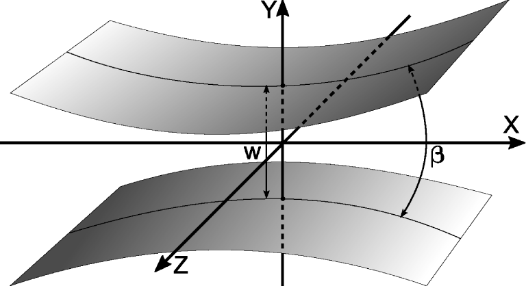
In this paper, we present theoretical and simulation studies of plasma channel formation in the line focus of a knife-like nanosecond duration laser pulse. The axis of the plasma channel is perpendicular to the direction of the knife-like laser beam propagation (see figure 1). When the focus and, hence, the plasma channel are long enough, then the latter can be used as a waveguide for high power femto-second laser pulses. An advantage of such a scheme is the possibility of, to some extent, arbitrarily lengthening the plasma channel, because different parts of the channel operate almost independently. As a result, we could add new sections of laser initiators along the plasma channel and lengthen the gas jet or the gas cell. Another advantage is that the longitudinal homogeneity of the channel is completely controlled by external conditions, and not by plasma processes. One of disadvantages is possible asymmetry of the channel in the plane perpendicular to its axis. One of the main goals of this work is to find conditions when this asymmetry is as low as possible. The laser pulse and initial gas parameter ranges considered here are based on the laser-generated plasma channel experiment (Levato et al. Reference Levato, Bonora, Grittani, Lazzarini, Nawaz, Nevrkla, Villanova, Ziano, Bassanese and Bobrova2018).
The surfaces show the edges of the laser pulse focused in the stripe of width  $w$. The focusing angle
 $\unicode[STIX]{x1D6FD}$ of the knife-like laser pulse is assumed to be small. The plasma channel will be formed along the
 $z$-axis. Its diameter will be typically larger than
 $w$.

When studying such plasma channels theoretically and in computer simulations, we assume that the channel is homogeneous along the line focus. However, we note that the experimental degree of this homogeneity should be high enough to ensure effective transportation of the high intensity laser pulse over long distances in such a plasma channel. As was mentioned above, the plasma channel should not only be homogeneous along the line focus, but also azimuthally symmetric in the transverse direction to avoid significant light scattering and seeding of unwanted instabilities. However, the electromagnetic field distribution in the focus of a knife-like laser pulse is not azimuthally symmetric, which should translate into azimuthal asymmetry of the plasma density. It is obvious that, for a longer focal length (or smaller convergence angle of laser pulse), the field asymmetry at focus is higher. It is plausible, however, that the heated plasma expansion might result in the channel symmetrization.
The two-dimensional (2-D) simulations are performed using the magnetohydrodynamic (MHD) computer code MARPLE, developed in the Keldysh Institute of Applied Mathematics (Gasilov et al. Reference Gasilov, Boldarev, Dyachenko, Olkhovskaya, Kartasheva, Bagdasarov, Boldyrev, Gasilova, Shmyrov, Tkachenko, De Bosschere, D’Hollander, Joubert, Padua and Peters2012). The code MARPLE is used to simulate capillary discharges with the parameters typical for the laser driven multi-GeV electron accelerators (Bagdasarov et al. Reference Bagdasarov, Sasorov, Gasilov, Boldarev, Olkhovskaya, Benedetti, Bulanov, Gonsalves, Mao and Schroeder2017a,Reference Bagdasarov, Sasorov, Boldarev, Olkhovskaya, Gasilov, Gonsalves, Barber, Bulanov, Schroeder and van Tilborgb,Reference Bagdasarov, Bobrova, Boldarev, Olkhovskaya, Sasorov, Gasilov, Barber, Bulanov, Gonsalves and Schroederc). It is also instrumental in studying the effects of laser heating of the capillary discharge plasma for optimization of the high power laser pulse guidance within the formed waveguide (Bobrova et al. Reference Bobrova, Sasorov, Benedetti, Bulanov, Geddes, Schroeder, Esarey and Leemans2013; Gonsalves et al. Reference Gonsalves, Nakamura, Daniels, Benedetti, Pieronek, de Raadt, Steinke, Bin, Bulanov and van Tilborg2019). The code was upgraded in order to take into account the heating of plasma by the inverse bremsstrahlung absorption in the focus of the laser pulse, so it can be used to simulate the plasma channel creation by the knife-like laser pulses. The distribution of the electromagnetic field at focus is obtained from the solution of Maxwell equations. This solution is then used to determine the laser energy deposition in the plasma in the MHD simulations of the plasma dynamics. Finally, the resulting local energy deposition is determined by both electromagnetic energy density and the distributions of plasma temperature and density.
The paper is organized as follows. In § 2, we formulate the model of the laser energy deposition in the plasma for sufficiently small convergence angles of the laser pulse. The simulation results are presented in § 3. They give the spatial distribution of the plasma parameters for different values of the convergence angle and laser pulse duration. We conclude in § 4.
2 Deposition of laser pulse energy in an under-critical density plasma
2.1 Spatial distribution of the electric field in the focus of a knife-like beam in an under-critical plasma
In order to determine the knife-like laser pulse energy deposition in the gas target, the electromagnetic field distribution in the focal region needs to be calculated. In figure 1 we show schematically the focusing of the laser pulse. We will assume later that the focusing angle of the laser pulse,  $\unicode[STIX]{x1D6FD}$, is small compared to unity.
Let us consider a stationary electromagnetic field in a vacuum. Assuming a 2-D geometry, all components of the electromagnetic field depend on time and on the coordinates  $x$ and
 $y$ only. The electric field in the focus region is
 $\boldsymbol{E}(\mathbf{x},t)=(E_{x},E_{y},E_{z})=(0,0,E(x,y)\exp (-\text{i}\unicode[STIX]{x1D714}t))$, where
 $\unicode[STIX]{x1D714}=kc$ is the frequency of the electromagnetic wave,
 $k=2\unicode[STIX]{x03C0}/\unicode[STIX]{x1D706}$ is the wavenumber and
 $\unicode[STIX]{x1D706}$ is the wavelength. This choice of electric field configuration corresponds to the transverse-electric (TE) polarization. The transverse-magnetic (TM) polarization can be considered in a similar way. The electric field
 $E$ is the solution of the Helmholtz equation (Landau & Lifshitz Reference Landau and Lifshitz1960)
 $$\begin{eqnarray}\unicode[STIX]{x1D6FB}^{2}E+k^{2}E=0.\end{eqnarray}$$
Here, the operator  $\unicode[STIX]{x1D735}$ acts in the 2-D space
 $(x,y)$, i.e.
 $\unicode[STIX]{x1D735}=(\unicode[STIX]{x2202}_{x},\unicode[STIX]{x2202}_{y},0)$. The
 $z$-component of the electric field is equal to real part of the complex value
 $E$.
The derivation of the exact solution of (2.1) for our set-up is presented in appendix A along with an approximate expression that is used in the simulations below. The distribution of  $|E|^{2}(x,y)$ depends on the laser wavelength and laser intensity, and on the focusing angle
 $\unicode[STIX]{x1D6FD}$ defined as full width at half maximum (FWHM) of the angular distribution of the intensity of the laser beam at sufficiently large distances from the focus. The approximation used corresponds to assuming
 $\unicode[STIX]{x1D6FD}$ to be small. However, we demonstrate in appendix A that it has reasonable accuracy up to
 $\unicode[STIX]{x1D6FD}=45^{\circ }$ when compared to the exact solution.
This approximate equation relates the electromagnetic energy flux  $F$ (measured in
 $\text{erg}~\text{s}^{-1}~\text{cm}^{-2}$),
 $|E|^{2}$ and
 $J(t)$ that is the intensity
 $J(t)$ of the knife-like laser pulse in terms of its power per unit length along the
 $z$-axis and measured in
 $\text{erg}~\text{s}^{-1}~\text{cm}^{-1}$. It is given by
 $$\begin{eqnarray}\displaystyle F & = & \displaystyle c\frac{|E|^{2}}{8\unicode[STIX]{x03C0}}\nonumber\\ \displaystyle & = & \displaystyle J(t)\,\frac{2\sqrt{\unicode[STIX]{x03C0}}\,\unicode[STIX]{x1D6FC}}{\sqrt{4\unicode[STIX]{x03C0}^{2}\unicode[STIX]{x1D6FC}^{4}x^{2}+\unicode[STIX]{x1D706}^{2}}}\exp \left(-\frac{4\unicode[STIX]{x03C0}^{2}\unicode[STIX]{x1D6FC}^{2}y^{2}}{4\unicode[STIX]{x03C0}^{2}\unicode[STIX]{x1D6FC}^{4}x^{2}+\unicode[STIX]{x1D706}^{2}}\right).\end{eqnarray}$$
For  $2\unicode[STIX]{x03C0}\unicode[STIX]{x1D6FC}|x|\gg \unicode[STIX]{x1D706}$ the dependence given by (2.2) corresponds to the Gaussian angular distribution of the radiation flux of the beam. The focusing angle
 $\unicode[STIX]{x1D6FD}$ (FWHM) of the laser pulse, expressed via the parameter
 $\unicode[STIX]{x1D6FC}$, is given by
 $$\begin{eqnarray}\unicode[STIX]{x1D6FD}=2\sqrt{\ln 2}\,\unicode[STIX]{x1D6FC}.\end{eqnarray}$$
Here, we assume that  $\unicode[STIX]{x1D6FC}$ and, hence,
 $\unicode[STIX]{x1D6FD}$ are much smaller than unity.
We neglect the finite difference of the refraction index of plasma from unity throughout this section. Such an approximation is reasonable if  $\unicode[STIX]{x1D6FC}\gg n_{e}/n_{\text{cr}}$. This strong inequality is satisfied for the range of densities considered in the present paper.
Although we take into account non-stationarity of the laser pulse, i.e. the dependence of  $J(t)$ on time
 $t$, as well as the propagation of the electromagnetic wave, the expression (2.2) does not take into account the effect of retardation. It can be neglected because
 $c\unicode[STIX]{x1D70F}$ is several orders of magnitude larger than
 $L_{x}$. Here,
 $\unicode[STIX]{x1D70F}$ is the duration of the laser pulse with a typical value of 2–10 ns in our simulations, and
 $L_{x}$ is the typical size of the hot plasma in the
 $x$-direction that will be of the order of a few hundred
 $\unicode[STIX]{x03BC}\text{m}$. In this case, the wave can be considered as stationary, although propagating.
The distribution (2.2) describes the pulse with transverse size  $w$ (FWHM) at focus, which is equal to
 $$\begin{eqnarray}w=\frac{\sqrt{\ln 2}}{\unicode[STIX]{x03C0}\,\unicode[STIX]{x1D6FC}}\,\unicode[STIX]{x1D706}\,,\end{eqnarray}$$
and determined by diffraction.
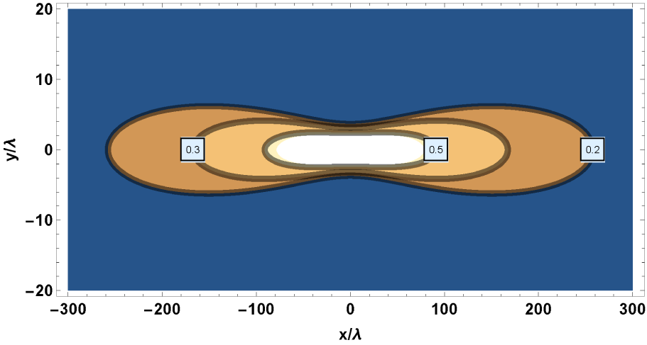
An example of the spatial distribution (2.2) of the laser energy flux is shown in figure 2 for  $\unicode[STIX]{x1D6FD}=5.2^{\circ }$.
The contours of constant value of  $F$ in the focus of a knife-like beam in the plane
 $(x/\unicode[STIX]{x1D706},y/\unicode[STIX]{x1D706})$ for a focusing angle of the laser pulse equal to
 $\unicode[STIX]{x1D6FD}=5.2^{\circ }$ (
 $m^{2}=1$). The contours correspond to 0.5, 0.3 and 0.2 of the maximum value at the point
 $(x=0,y=0)$. The beam propagates in the
 $x$-direction. The field distribution has different scales for
 $x$- and
 $y$-axes.

Equation (2.2), as well as the theory developed to derive it, are obtained for an ideally spatially coherent laser pulse, i.e. it can be described as a single transverse mode in terms of (A 7). The laser pulses in the experiment might not satisfy the condition of ideal coherence. If an incoherent beam has the same direction of propagation and the same focusing angle, then it can be considered as an incoherent sum of coherent laser pulses with different  $y$-positions of their foci. If we assume additionally that the beam preserves a Gaussian form, then (2.2) and (2.4) can be rewritten with the following substitution:
 $\unicode[STIX]{x1D706}\rightarrow m^{2}\unicode[STIX]{x1D706}$, where
 $m^{2}$ is the so-called
 $m^{2}$-parameter, describing the ‘quality’ of the laser pulse in terms of its coherence (Siegman Reference Siegman1993). As a result, these equations may be rewritten in the form
 $$\begin{eqnarray}\displaystyle F & = & \displaystyle c\frac{|E|^{2}}{8\unicode[STIX]{x03C0}}=J(t)\,\frac{2\sqrt{\unicode[STIX]{x03C0}}\,\unicode[STIX]{x1D6FC}}{\sqrt{4\unicode[STIX]{x03C0}^{2}\unicode[STIX]{x1D6FC}^{4}x^{2}+m^{4}\unicode[STIX]{x1D706}^{2}}}\nonumber\\ \displaystyle & & \displaystyle \times \,\exp \left(-\frac{4\unicode[STIX]{x03C0}^{2}\unicode[STIX]{x1D6FC}^{2}y^{2}}{4\unicode[STIX]{x03C0}^{2}\unicode[STIX]{x1D6FC}^{4}x^{2}+m^{4}\unicode[STIX]{x1D706}^{2}}\right),\end{eqnarray}$$
 $$\begin{eqnarray}w=\frac{\sqrt{\ln 2}}{\unicode[STIX]{x03C0}\unicode[STIX]{x1D6FC}}m^{2}\unicode[STIX]{x1D706}.\end{eqnarray}$$
A Gaussian beam, or, in general, a converging laser pulse, is defined completely by  $J(t)$,
 $\unicode[STIX]{x1D706}$,
 $\unicode[STIX]{x1D6FC}$ and
 $m^{2}$ in the framework of our model.
2.2 Laser energy deposition rate in the plasma
For a given spatial distribution of the laser pulse intensity,  $cE^{2}/8\unicode[STIX]{x03C0}$, in the focal region, which is a function of
 $(x,y,z,t)$, the inverse bremsstrahlung absorption in the plasma is described by an imaginary part of the permittivity:
 $\unicode[STIX]{x1D700}=\unicode[STIX]{x1D700}^{\prime }+\text{i}\unicode[STIX]{x1D700}^{\prime \prime }$. We assume that the plasma density is under-critical, i.e.
 $n_{e}\ll n_{e\,\text{cr}}$. The rate of plasma heating due to finite
 $\unicode[STIX]{x1D700}^{\prime \prime }$ is given by the expression (Landau & Lifshitz Reference Landau and Lifshitz1960; Lifshitz & Pitaevskii Reference Lifshitz and Pitaevskii2002)
 $$\begin{eqnarray}Q=\frac{|E|^{2}}{8\unicode[STIX]{x03C0}}\unicode[STIX]{x1D714}\unicode[STIX]{x1D700}^{\prime \prime }=\frac{|E|^{2}}{8\unicode[STIX]{x03C0}}c\,\frac{2\unicode[STIX]{x03C0}\unicode[STIX]{x1D700}^{\prime \prime }}{\unicode[STIX]{x1D706}}=F\,\frac{2\unicode[STIX]{x03C0}\unicode[STIX]{x1D700}^{\prime \prime }}{\unicode[STIX]{x1D706}}.\end{eqnarray}$$
The function  $F$ is given by (A 17). The imaginary part of the permittivity,
 $\unicode[STIX]{x1D700}^{\prime \prime }$, for the inverse bremsstrahlung process (Lifshitz & Pitaevskii Reference Lifshitz and Pitaevskii2002), is equal to
 $$\begin{eqnarray}\unicode[STIX]{x1D700}^{\prime \prime }=\frac{4\sqrt{2\unicode[STIX]{x03C0}}}{3}\frac{ze^{4}n_{e}}{m_{e}^{1/2}T_{e}^{3/2}}\,\frac{\unicode[STIX]{x1D714}_{pe}^{2}}{\unicode[STIX]{x1D714}^{3}}\unicode[STIX]{x1D6EC},\end{eqnarray}$$
where
 $$\begin{eqnarray}\unicode[STIX]{x1D6EC}=\max \left\{\frac{\unicode[STIX]{x03C0}}{\sqrt{3}},\frac{1}{2}\ln \frac{2^{5}T_{e}^{3}}{e^{5\unicode[STIX]{x1D6FE}}\unicode[STIX]{x1D714}^{2}z^{2}e^{4}m_{e}}\right\}.\end{eqnarray}$$
Here,  $e$ and
 $m_{e}$ are the charge and the mass of an electron, respectively,
 $T_{e}$ and
 $n_{e}$ are the temperature and the density of the electrons,
 $z$ is the mean ion charge,
 $\unicode[STIX]{x1D714}_{pe}=\sqrt{4\unicode[STIX]{x03C0}n_{e}e^{2}/m_{e}}$ is the plasma frequency and
 $\unicode[STIX]{x1D6FE}=0.57721\ldots$ is the Euler constant. This expression for the rate of plasma heating due to the absorption of the laser pulse energy via the inverse bremsstrahlung process is valid when
 $T_{e}\ll z^{2}e^{4}m_{e}/\hbar ^{2}\sim 27z^{2}$ eV and
 $\unicode[STIX]{x1D714}\gg \unicode[STIX]{x1D714}_{pe}$ (Sobelman Reference Sobelman1992; Lifshitz & Pitaevskii Reference Lifshitz and Pitaevskii2002).
We note that the expressions (2.7)–(2.9) are obtained assuming full ionization of the plasma. In the case of a partially ionized plasma, these expressions should be modified by changing  $z^{3}$ to
 $z_{1}z^{2}$ in (2.8), and
 $z^{2}$ to
 $z_{1}^{2}$ in (2.9), where
 $z_{1}=\max \{1,z\}$.
The expressions (2.7)–(2.9) say that a laser beam with a wavelength of  $\unicode[STIX]{x1D706}=1.03~\unicode[STIX]{x03BC}\text{m}$ has an absorption coefficient
 $2\unicode[STIX]{x1D700}^{\prime \prime }/\unicode[STIX]{x1D706}\simeq 1.4\times 10^{-2}~\text{cm}^{-1}$ in a fully ionized hydrogen plasma with electron density,
 $n_{e}=3\times 10^{18}~\text{cm}^{-3}$, and temperature,
 $T_{e}=15$ eV. It means that deposited power per unit volume,
 $Q$, is equal to
 $Q\simeq 1.8~\text{GW}~\text{cm}^{-3}$ for the laser beam with total energy per unit length along the
 $z$-axis,
 $J_{\text{tot}}=10~\text{J}~\text{cm}^{-1}$, duration of 8 ns and
 $w=10~\unicode[STIX]{x03BC}\text{m}$.
We implement the above described absorption model in the computer code MARPLE. This model was used to simulate the effects of the laser heating in Gonsalves et al. (Reference Gonsalves, Nakamura, Daniels, Benedetti, Pieronek, de Raadt, Steinke, Bin, Bulanov and van Tilborg2019), Bobrova et al. (Reference Bobrova, Sasorov, Benedetti, Bulanov, Geddes, Schroeder, Esarey and Leemans2013) and Ragozin et al. (Reference Ragozin, Levashov, Mednikov, Pirozhkov, Sasorov, Khounsary and MacDonald2002). The agreement between the results of the simulations and the experimental results, reported by Gonsalves et al. (Reference Gonsalves, Nakamura, Daniels, Benedetti, Pieronek, de Raadt, Steinke, Bin, Bulanov and van Tilborg2019) and Ragozin et al. (Reference Ragozin, Levashov, Mednikov, Pirozhkov, Sasorov, Khounsary and MacDonald2002), was demonstrated.
If the parameter  $\unicode[STIX]{x1D6FC}$ of the laser pulse is much less than unity, and much larger than the ratio
 $n_{e}/n_{e\,\text{cr}}$, i.e.
 $1\gg \unicode[STIX]{x1D6FC}\gg n_{e}/n_{e\,\text{cr}}$, then the refraction effects are negligibly small. Here,
 $n_{e\,\text{cr}}=m_{e}\unicode[STIX]{x1D714}^{2}/4\unicode[STIX]{x03C0}e$ is the critical plasma density. We neglect also the depletion of the laser pulse energy due to the inverse bremsstrahlung absorption in the focus region.
If the laser pulse propagates along the  $x$-axis, where the laser pulse intensity does not depend on the coordinate
 $z$, then at each moment in time we can find the peak value of
 $F$, which is equal to
 $$\begin{eqnarray}F_{0}(t)=J(t)\frac{2\sqrt{\unicode[STIX]{x03C0}}\unicode[STIX]{x1D6FC}}{\unicode[STIX]{x1D706}}.\end{eqnarray}$$
3 Two-dimensional gas-dynamics simulations of plasma channel formation
3.1 Main physical parameters of simulations
Here, we discuss the simulations of a plasma channel formation, elongated in the  $z$ direction by a knife-like laser pulse propagating in the
 $x$-direction. Thus, the laser beam propagates perpendicular to the forming plasma channel. The channel is formed in an ambient gas, with an initially homogeneous density. The laser pulse is assumed to be homogeneous along the
 $z$-axis, and is focused onto the line
 $x=y=0$. Near the focus the distribution of the knife-like laser pulse energy flux,
 $F(x,y,t)$, taking into account the diffraction, is described in § 2.1 (equation (2.5)). We set the following dependence of the laser power on time:
 $$\begin{eqnarray}J(t)=\left\{\begin{array}{@{}ll@{}}J_{\text{tot}}\unicode[STIX]{x1D70F}^{-1}\sin ^{2}(\unicode[STIX]{x03C0}t/2\unicode[STIX]{x1D70F})\quad & \text{for }0<t<2\unicode[STIX]{x1D70F}\\ 0\quad & \text{for }t>2\unicode[STIX]{x1D70F},\end{array}\right.\end{eqnarray}$$
per unit length in the  $z$-direction. Thus, the laser pulse, forming the plasma channel, is characterized by the following five parameters: (i)
 $\unicode[STIX]{x1D706}=2\unicode[STIX]{x03C0}c/\unicode[STIX]{x1D714}$, wavelength of the laser, (ii)
 $J_{\text{tot}}$, total energy of the laser pulse per unit length in the
 $z$-direction; (iii)
 $\unicode[STIX]{x1D70F}$, duration (FWHM) of the laser pulse; (iv)
 $\unicode[STIX]{x1D6FD}$, focusing angle (FWHM) of the laser pulse in the plane
 $(x,y)$; and (v)
 $m^{2}$. We set
 $\unicode[STIX]{x1D706}=1030$ nm,
 $J_{\text{tot}}=12~\text{J}~\text{cm}^{-1}$ and
 $m^{2}=1$ for all simulations, varying
 $\unicode[STIX]{x1D70F}$ and
 $\unicode[STIX]{x1D6FD}$.
The ambient gas is hydrogen with an initial density of  $24~\unicode[STIX]{x03BC}\text{g}~\text{cm}^{-3}$ and temperature of 0.3 eV. The hydrogen gas was chosen for our simulations because it can be fully ionized at moderate plasma temperatures of several eV, and because it was used in recent LWFA experiments as a target (Leemans et al. Reference Leemans, Gonsalves, Mao, Nakamura, Benedetti, Schroeder, Tóth, Daniels, Mittelberger and Bulanov2014; Gonsalves et al. Reference Gonsalves, Nakamura, Daniels, Benedetti, Pieronek, de Raadt, Steinke, Bin, Bulanov and van Tilborg2019). The optical breakdown of hydrogen by the laser pulse is initiated by a spark in a small vicinity of the line
 $x=y=0$. This is necessary because the physical model used in the code does not include several physical processes important for optical breakdown. We do not specify here the parameters of the spark, such as its temperature and size, assuming that the final parameters of the plasma channel do not depend on them, provided the breakdown takes place in a short period after the laser pulse onset.
In what follows we use the 3-D MHD code MARPLE to model the process of laser heating and plasma channel formation. The physical model implemented in this code is described in appendix B. Although the model includes the full set of MHD equations, only the part that describes the dynamics of the gas is used in our simulations. We also utilize the model of the laser beam energy deposition described in § 2. The code is designed to use the finite volume technique on general unstructured simulation meshes and a parallel computation technique with message passing communications. It was successfully used to model several experiments. These include experiments on laser wake field accelerators of electrons in capillary discharges (Bagdasarov et al. Reference Bagdasarov, Sasorov, Gasilov, Boldarev, Olkhovskaya, Benedetti, Bulanov, Gonsalves, Mao and Schroeder2017a,Reference Bagdasarov, Sasorov, Boldarev, Olkhovskaya, Gasilov, Gonsalves, Barber, Bulanov, Schroeder and van Tilborgb,Reference Bagdasarov, Bobrova, Boldarev, Olkhovskaya, Sasorov, Gasilov, Barber, Bulanov, Gonsalves and Schroederc; Gonsalves et al. Reference Gonsalves, Nakamura, Daniels, Benedetti, Pieronek, de Raadt, Steinke, Bin, Bulanov and van Tilborg2019), experiments with dense Z-pinches formed by multi-wire arrays in pulsed power facilities (Grabovski et al. Reference Grabovski, Aleksandrov, Volkov, Gasilov, Gribov, Gritsuk, Dyachenko, Zaitsev, Medovshchikov and Mitrofanov2008; Aleksandrov et al. Reference Aleksandrov, Gasilov, Grabovski, Gritsuk, Laukhin, Mitrofanov, Oleinik, Olkhovskaya, Sasorov and Smirnov2014, Reference Aleksandrov, Branitski, Gasilov, Grabovskiy, Gritsuk, Mitrofanov, Olkhovskaya, Sasorov and Frolov2019; Olkhovskaya et al. Reference Olkhovskaya, Basko, Sasorov, Vitchev, Novikov, Boldarev, Gasilov and Tkachenko2015) and experiments on the solid matter response to high intensity electron beams (Ananyev et al. Reference Ananyev, Bagdasarov, Danko, Demidov, Kazakov, Kalinin, Kurilo, Olkhovskaya, Strizhakov and Gasilov2017; Gasilov et al. Reference Gasilov, Grushin, Ermakov, Olkhovskaya and Petrov2019), etc.
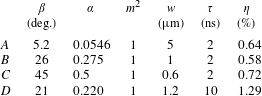
We performed four different simulations. The parameters of the laser beam that were varied in these simulations are presented in table 1. Section 3.2 is devoted to the general description of the simulated dynamics of plasma channel formation under these conditions and to the investigation of the dependence of plasma channel parameters on the focusing angle  $\unicode[STIX]{x1D6FD}$ of the laser pulse. Section 3.3 is devoted to the investigation of the effects of the laser pulse duration,
 $\unicode[STIX]{x1D70F}$.
3.2 Dependence of plasma channel parameters on the focusing angle  $\unicode[STIX]{x1D6FD}$ of the laser pulse

3.2.1 Simulation set-up
We perform four simulations ( $A$,
 $B$,
 $C$ and
 $D$) with different values of
 $\unicode[STIX]{x1D6FD}$ and
 $\unicode[STIX]{x1D70F}$, whereas other physical parameters remain fixed (see table 1). We assume that the minimum size
 $w$ of the spatial distribution of the laser pulse energy in the
 $(x,y)$-plane is limited by diffraction only for the initial beam, as was described in § 2.1, and hence depends significantly on the focusing angle of the beam,
 $\unicode[STIX]{x1D6FD}$, as shown in table 1. An example of the spatial distribution of the laser intensity in the
 $(x,y)$-plane for the simulation
 $A$ (
 $\unicode[STIX]{x1D6FD}=5.2^{\circ }$) is shown in figure 2.
Parameters of the 2-D simulations and simulated percentages of laser energy  $\unicode[STIX]{x1D702}$ deposited into the plasma.

In this section we study how the knife-like nanosecond laser pulse structure affects the azimuthal symmetry of the plasma channel. We perform three simulations,  $A$,
 $B$ and
 $C$, with different values of
 $\unicode[STIX]{x1D6FD}$,
 $\unicode[STIX]{x1D6FD}=5.2^{\circ }$,
 $26^{\circ }$ and
 $45^{\circ }$, for
 $\unicode[STIX]{x1D70F}=2$ ns. The laser pulse duration is chosen to be relatively small since it is plausible to assume that the hydrodynamic expansion of the heated plasma channel outward into the homogeneous ambient gas might lead to the symmetrization of initially asymmetric energy deposition by the laser pulse (e.g. see figure 2).
In the  $A$ and
 $B$ cases the simulation box is
 $2~\text{mm}\times 2~\text{mm}$ or in the
 $(x,y)$-plane
 $[-1~\text{mm};+1~\text{mm}]\times [-1~\text{mm};+1~\text{mm}]$. We use two-dimensional grids, composed of rectangular cells, for the spatial discretization. These two-dimensional grids are the products of two one-dimensional grids. The grid mesh size varies from 250 nm (case
 $A$) and 50 nm (case
 $B$) in the vicinity of the axis
 $(x=0,y=0)$ to
 $100~\unicode[STIX]{x03BC}\text{m}$ and
 $25~\unicode[STIX]{x03BC}\text{m}$, respectively, near the simulation box boundary. The total number of cells is
 $600\times 600$ in case
 $A$ and
 $2700\times 2700$ in case
 $B$. The following symmetries can be applied in the simulations
 $x\rightarrow -x$ and
 $y\rightarrow -y$ in order to reduce the computational load. The
 $x\rightarrow -x$ symmetry is due to the fact that we neglect the effect of the laser depletion because of the absorption (see the estimates below). In case
 $C$, the simulation box is
 $1~\text{mm}\times 1~\text{mm}$ or in the
 $(x,y)$-plane:
 $[0;\,1~\text{mm}]\times [0;1~\text{mm}]$, which is a quarter of the simulation box used in cases
 $A$ and
 $B$. The solution in the whole domain
 $2~\text{mm}~\times 2~\text{mm}$ is obtained by using the
 $x\rightarrow -x$ and
 $y\rightarrow -y$ symmetries. The smallest grid mesh size is equal to 50 nm in the vicinity of the axis
 $(x=0,y=0)$. The largest grid mesh size is equal to
 $25~\unicode[STIX]{x03BC}\text{m}$ in the vicinity of the outer boundary. The total number of cells is equal to
 $1400\times 1400$. The simulation
 $A$ is performed for the time interval
 $t\in [0,10~\text{ns}]$, whereas the simulations
 $B$ and
 $C$ are performed for the time interval
 $t\in [0,15~\text{ns}]$.
3.2.2 Results of the simulations $A$, $B$ and $C$


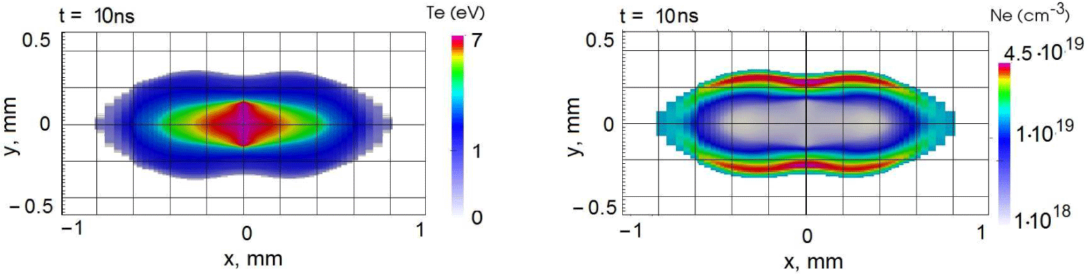
The results of the simulation  $A$ (
 $\unicode[STIX]{x1D6FD}=5.2^{\circ }$) are shown in figure 3, where the snapshots of the electron temperature,
 $T_{e}$, and the electron density,
 $N_{e}$, are presented at
 $t=10$ ns. It is clearly seen that the hot plasma bubble is asymmetric. See also § 3.4. Approximately 0.64 % of the total energy of the laser pulse is absorbed in the focus region. This number depends strongly on the dynamics of the plasma in and around the focus region during the laser pulse interaction with the target.
Snapshots of spatial distributions of electron temperature,  $T_{e}$, in eV and density,
 $N_{e}$, in cm
 $^{-3}$ at
 $t=10$ ns for the simulation
 $A$ (
 $\unicode[STIX]{x1D6FD}=5.2^{\circ }$,
 $\unicode[STIX]{x1D70F}=2$ ns).

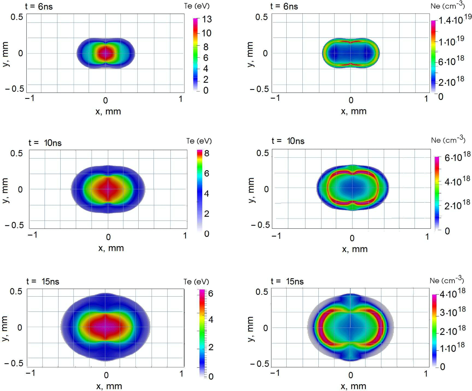
We now proceed to a more detailed presentation of the results of the  $B$ case (
 $\unicode[STIX]{x1D6FD}=26^{\circ }$). Figures 4 and 5 show the process of the hot (almost completely ionized) plasma bubble formation. In figure 4 we present the sequential snapshots of the electron temperature and density distributions in the
 $(x,y)$-plane at
 $t=6$, 10 and 15 ns. The electron density distribution near the axis
 $x=y=0$ becomes more symmetric than in the case
 $A$. The degree of symmetry of the electron density depression is considered below and can be seen in figure 8. The improved symmetry of the plasma channel is beneficial for guiding of high power laser pulses over a sufficiently long distance. The simulation shows that approximately 0.58 % of the total energy of the laser pulse is absorbed in the focus.
Snapshots of the spatial distribution of the electron temperature (eV) and density ( $\text{cm}^{-3}$) in the case
 $B$ (
 $\unicode[STIX]{x1D6FD}=26^{\circ }$,
 $\unicode[STIX]{x1D70F}=2$ ns) at
 $t=6$, 10 and
 $15$ ns, showing the blowing up of the hot plasma bubble.

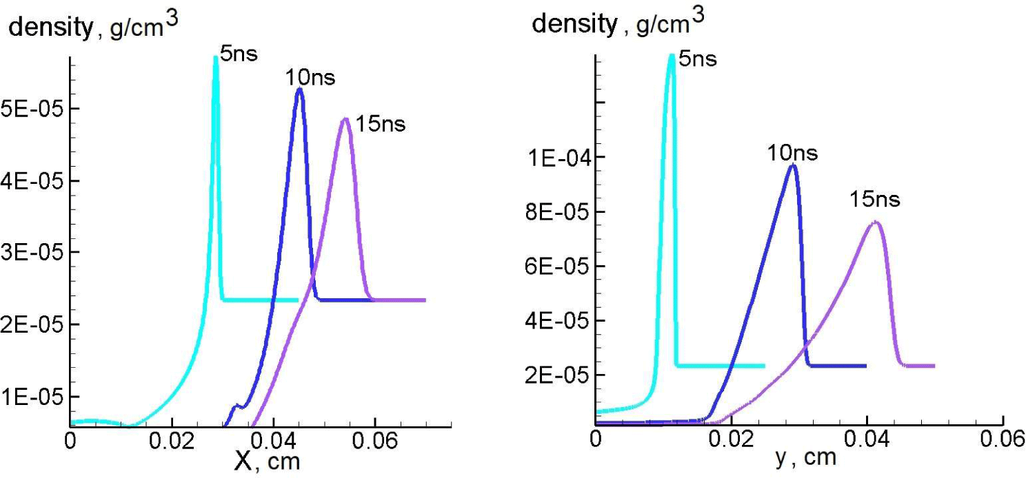
Shown are the plasma mass density distributions along the axis  $y=0$ and
 $x=0$ at
 $t=5,10,15$ ns for the simulation
 $B$ (
 $\unicode[STIX]{x1D6FD}=26^{\circ }$;
 $\unicode[STIX]{x1D70F}=2$ ns).

Snapshots of distribution of the plasma velocity components  $v_{x}$ (a),
 $v_{y}$ (b) and the
 $z$-component of plasma velocity curl
 $(\unicode[STIX]{x1D735}\times \boldsymbol{v})_{z}$ (c) measured in
 $10^{6}~\text{s}^{-1}$ at
 $t=15$ ns for the simulation
 $B$ (
 $\unicode[STIX]{x1D6FD}=26^{\circ }$;
 $\unicode[STIX]{x1D70F}=2$ ns).

In figure 5 we show the shock wave propagating outwards from the hot bubble. The shock wave is manifested by the typical distribution of the mass density along the  $x$- and
 $y$-directions at subsequent moments in time (see figure 5). If we define a boundary of the hot ionized plasma bubble as a position of maximum of the electron density along the radius, then the simulation shows that the shock wave encircles the area, which at
 $t=10$ ns is wider than the plasma bubble by approximately
 $100{-}150~\unicode[STIX]{x03BC}\text{m}$ in all directions. Since this distance is not substantially large compared to the bubble size, the shock wave is tightly attached to the hot bubble until the time
 $t=10$ ns. As a result, the homogeneous gas ahead of the shock wave front serves as a mitigating factor for the growing asymmetry. For sufficiently late times, when the shock wave outruns the growing bubble, this mitigating factor vanishes.
At  $t=10$ ns the electron temperature behind the shock wave is of the order of 1.5 eV. As a result, the degree of ionization is low. Hence, the hot bubble expands mainly due to the effect of thermal conductivity after the interaction with the laser pulse is over.
In order to explain the importance of the vortical motion of the plasma in the  $(x,y)$-plane we show the velocity field distribution at
 $t=15$ ns for the case
 $B$ in figure 6. Figure 6(a,b) show the distributions of the
 $y$ and
 $x$ components of the plasma velocity
 $\boldsymbol{v}$, respectively. Figure 6(c) shows the
 $z$-component of the vorticity
 $\unicode[STIX]{x1D74E}=\unicode[STIX]{x1D735}\times \boldsymbol{v}$ at the same time. The vorticity is generated due to two similar effects. Let us first mention that the vorticity is generated at the not perfectly plane shock wave front. The second source of the vorticity is the baroclinic effect
 $\unicode[STIX]{x1D735}p\times \unicode[STIX]{x1D735}\unicode[STIX]{x1D70C}\neq 0$, which takes place right behind the shock wave at its downstream side. Here,
 $p$ is the plasma pressure, and
 $\unicode[STIX]{x1D70C}$ is its mass density.
The typical value of the vorticity  $\unicode[STIX]{x1D714}_{z}$ is equal to
 $|\unicode[STIX]{x1D735}\times \boldsymbol{v}|\sim (0.5-1)\times 10^{8}~\text{s}^{-1}$ within the region
 $r=\sqrt{x^{2}+y^{2}}\lesssim 0.4$ mm. Assuming that the viscosity is relatively low, the vorticity
 $\unicode[STIX]{x1D714}_{z}$ is frozen into the plasma in accordance with Kelvin’s circulation theorem. This means that the plasma in the bubble turns inside out over approximately 30 ns. This will lead to the turbulent mixing of the plasma inside the bubble and to the distortion of the symmetric channel. This process prevents the azimuthal symmetrization of the plasma channel. Taking this into account, we stop the simulation at
 $t=20$ ns. The same conclusions can be drawn for all our simulation cases. The process of distortion of symmetric hot channels due to baroclinic vorticity generation and gas cooling was investigated earlier (see Kurzweil, Livne & Meerson Reference Kurzweil, Livne and Meerson2003, and references cited therein).
Let us consider the degree of asymmetry of the electron density depression near the axis of the plasma channel, in the region  $r<150~\unicode[STIX]{x03BC}\text{m}$. This region could be relevant for laser pulse guidance along the
 $z$-axis. We characterize the asymmetry by the difference between
 $N_{e}(r,0)$ and
 $N_{e}(0,r)$ at
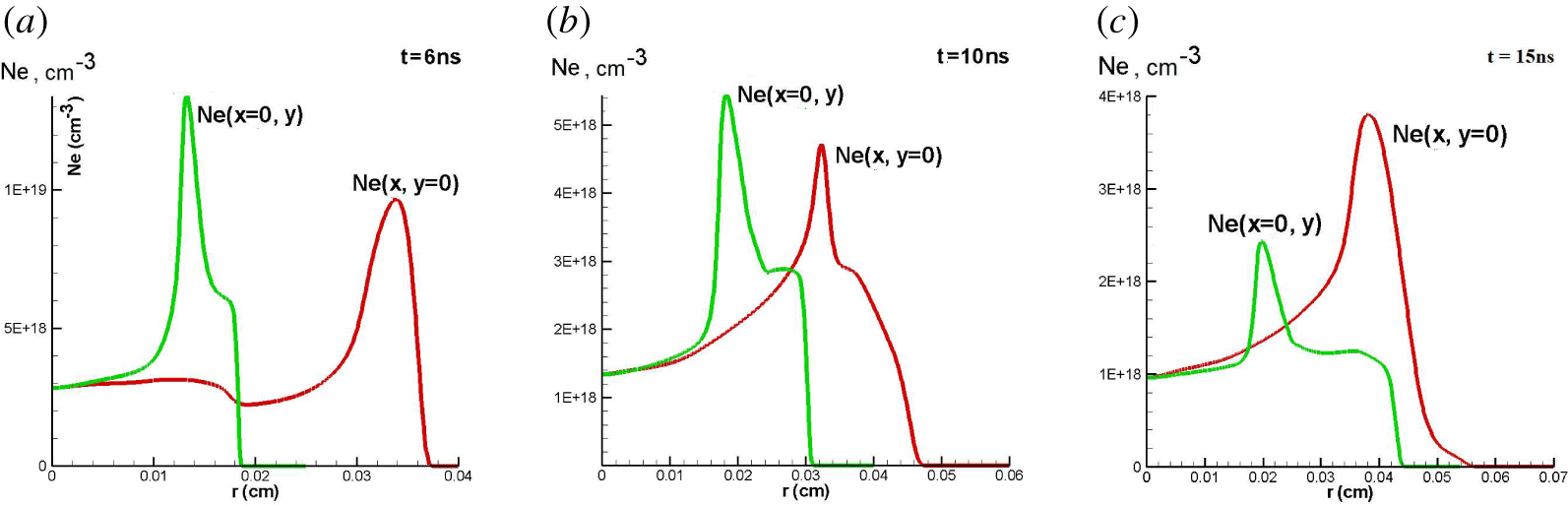
 $r\leqslant 150~\unicode[STIX]{x03BC}\text{m}$. A more specified definition of the asymmetry could be introduced after consideration of the propagation of laser pulses in the plasma channel, which is outside the scope of the present work. Figure 8 shows snapshots of 1-D distributions of electron density along the lines
 $x=0$ and
 $y=0$. The moments of the snapshots correspond to times
 $t=6$, 10 and 15 ns. The curves at
 $t<6$ ns and at
 $t>15$ ns behave like those at
 $t=6$ and 15 ns, respectively. We may see the electron density on the line
 $x=0$ is higher at
 $t=10$ ns than on the line
 $y=0$ at
 $r\lesssim 150~\unicode[STIX]{x03BC}\text{m}$, whereas they change ordering at
 $t=15$ ns. It means that the angular asymmetry at
 $r\lesssim 150~\unicode[STIX]{x03BC}\text{m}$ changes its sign during the period 10 ns
 ${<}t<15$ ns. It is plausible to assume that the optimal time for the laser pulse guiding through this plasma channel is in the interval
 $10~\text{ns}<t<15~\text{ns}$. The existence of such an optimal time seems to be the consequence of the vortex motion in the bubble, considered above. In this case, the continuation of the simulation to later times,
 $t>15$ ns, is not reasonable. The general conclusions presented in the latter three paragraphs could be applied with some quantitative corrections to all our simulations.
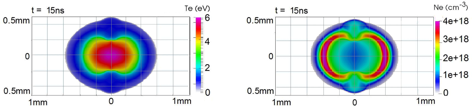
We present the results of simulation case  $C$ (
 $\unicode[STIX]{x1D6FD}=45^{\circ }$) in figures 7 and 13 (in § 3.4), which show the structure of the plasma channel at
 $t=15$ ns, and asymmetry of the depression of the electron density near its centre
 $(x,y)=(0,0)$ at the same time, respectively. The distribution of the electron density in the vicinity of the axis
 $x=y=0$ at the time
 $t=15$ ns becomes much more symmetric than in the case
 $A$, whereas the difference from case
 $B$ is not so significant.
Snapshots of spatial distribution of electron density ( $\text{cm}^{-3}$) and temperature (eV) for the simulation
 $C$ (
 $\unicode[STIX]{x1D6FD}=45^{\circ }$,
 $\unicode[STIX]{x1D70F}=2$ ns) at
 $t=15$ ns.

Time evolution of 1-D cross-sections of electron density distributions for the case  $B$ (
 $\unicode[STIX]{x1D6FD}=26^{\circ }$;
 $\unicode[STIX]{x1D70F}=2$ ns). The green lines correspond to the ray
 $x=0$,
 $y>0$ and the red lines do the ray
 $y=0,x>0$. (a–c) panels correspond to snapshots at
 $t=6$, 10 and 15 ns, respectively. Only the region
 $r\leqslant 150~\unicode[STIX]{x03BC}\text{m}$ may be relevant for possible wave guiding along the
 $z$-axis. Note the green lines are above the red lines in this region at
 $t=4$ and 6 ns, and they change ordering at
 $t=15$ ns. It indicates a change of sign of the azimuthal asymmetry in the electron density spatial distribution during the time
 $t\in (10,15)$ ns.

The simulation shows that approximately 0.72 % of the total laser pulse energy is absorbed in the focus region.
The waist size  $w$ of our laser beam is considerably less that the plasma bubble. To clarify this point we can compare
 $w$ from table 1 and the typical size of the hot plasma bubble for this case
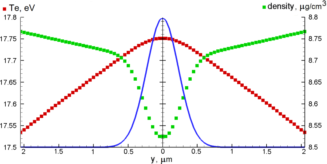
 $C$, presented in figure 7. Our non-equidistant simulation grid, described in § 3.2.1, allows us to resolve well the transverse size of laser energy deposition together with total size of the problem, keeping a reasonable number of meshes. To demonstrate the sufficient spatial resolution we show the spatial distribution of laser energy flux at the plane
 $x=0$ together with sets of grid values of electron temperature,
 $T_{e}$, and plasma density,
 $\unicode[STIX]{x1D70C}$, in figure 9.
The transverse distribution of the laser beam intensity (blue line, arbitrary units), electron temperature (red squares) and plasma density (green squares) at  $x=0$ at the moment of maximum intensity of the laser beam. The scales of the vertical axes are chosen to emphasize visible gradients. Actually
 $T_{e}$ and
 $\unicode[STIX]{x1D70C}$ are almost constant at spatial scales determined by the spot size of the laser focus.

3.3 Dependence of plasma channel on laser pulse duration
3.3.1 Simulation set-up
In what follows we present the results of simulations of the case  $D$ (
 $\unicode[STIX]{x1D6FD}=21^{\circ }$,
 $\unicode[STIX]{x1D70F}=10$ ns) from table 1. The general structure of the simulation box is similar to the case
 $B$ in § 3.2. The smallest grid mesh size is equal to 125 nm in the vicinity of the axis
 $(x,y)=(0,0)$, and the largest one is equal to
 $100~\unicode[STIX]{x03BC}\text{m}$ in the vicinity of the outer boundary at
 $x=2$ mm. The total number of points of the two-dimensional grid is
 $872\times 851=742\,072$. The simulation is performed for the time interval
 $t\in [0;20~\text{ns}]$, so that the peak of the laser pulse reaches the focus at
 $t=10$ ns.
3.3.2 Results of the simulation $D$

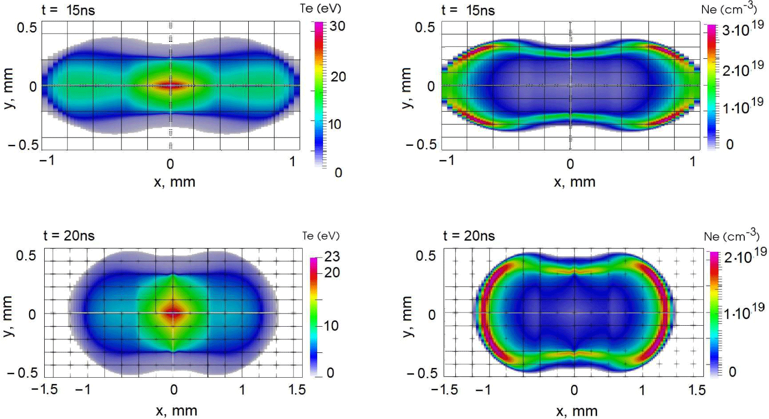
Snapshots of the electron temperature (eV) and density ( $\text{cm}^{-3}$) spatial distributions at
 $t=15$ and 20 ns in the case
 $D$ (
 $\unicode[STIX]{x1D6FD}=21^{\circ }$;
 $\unicode[STIX]{x1D70F}=10$ ns).

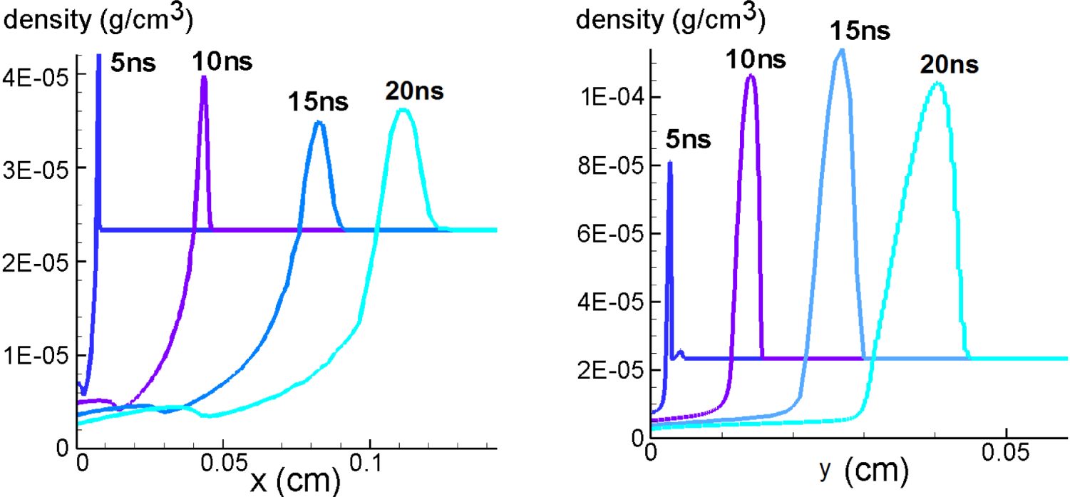
Mass density distributions along the  $x$- and
 $y$-axes at different time moments in the case
 $D$ (
 $\unicode[STIX]{x1D6FD}=21^{\circ }$;
 $\unicode[STIX]{x1D70F}=10$ ns).

The results of the simulation of case  $D$ are summarized in figures 10–13 (in § 3.4). Figure 10 shows the 2-D distributions of electron temperature,
 $T_{e}$, and electron density,
 $N_{e}$, on the plane
 $(x,y)$ at
 $t=15$ ns. The plasma channel is elongated in the
 $x$-direction, which is the direction of laser pulse propagation.
Figure 11 shows the dependences of the plasma density,  $\unicode[STIX]{x1D70C}$, measured in
 $\text{g}~\text{cm}^{-3}$, along the
 $y$ axis,
 $(x=0,y>0)$, and along the
 $x$ axis,
 $(x>0,y=0)$, at
 $t=5$, 10, 15 and 20 ns. It demonstrates the strong shock wave propagation outside the region of the laser energy deposition, and the formation of a hot plasma bubble inside the low density region. It is interesting to compare the size of the hot bubble with the size of the region bounded by the shock wave at
 $t=15$ ns. We define the hot bubble as the region where the temperature
 $T_{e}$ is higher than half of the maximum temperature at
 $x=y=0$. If we compare the curves in figure 11, corresponding to
 $t=15$ ns, with the upper row in figure 10, we can see that the typical size of the plasma bubble in both directions of its symmetry is approximately 1.5–2 times smaller than the size of the region bounded by the shock wave. The position of the shock wave at the line
 $y=0$ moves outward faster than the analogous position of the shock wave on the line
 $x=0$. This effect is caused by the additional heating and ionization of relatively cold plasma behind the shock wave front in the vicinity of the line
 $y=0$ by the laser pulse. Such additional heating takes place due to the enhanced energy deposition from the laser pulse in this region. This effect is more important than the effect of the higher plasma pressure gradient in the
 $y$-direction. We conclude that the ionization front, moving in the
 $x$-direction, is driven mainly by the additional plasma heating, whereas the shock wave moving in this direction, and accompanying the ionization front, is more or less a secondary effect. It is necessary to note that the effect of the faster plasma front propagation in the
 $x$-direction is influenced considerably by the significant 2-D structure of motion at the tip of the shock wave along the
 $y=0$ line.
From the comparison of figures 10 and 11, one can see the maximum temperature is accompanied by the electron density minimum, at the centre  $(x,y)=(0,0)$. We note that hydrogen is almost completely ionized at
 $T_{e}>5$ eV. Hence, the distribution of
 $N_{e}$ corresponds actually to the distribution of mass density,
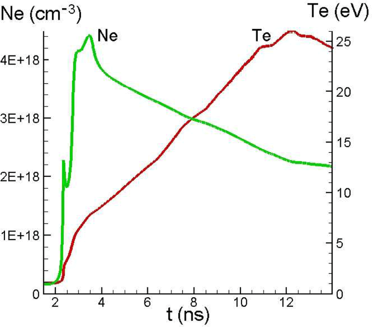
 $\unicode[STIX]{x1D70C}$. Time dependencies of
 $T_{e}$ and
 $N_{e}$ maxima are presented in figure 12.
Time dependencies of electron density  $N_{e}(0,0,t)$ and temperature
 $T_{e}(0,0,t)$ in the case
 $D$ (
 $\unicode[STIX]{x1D6FD}=21^{\circ }$;
 $\unicode[STIX]{x1D70F}=10$ ns).

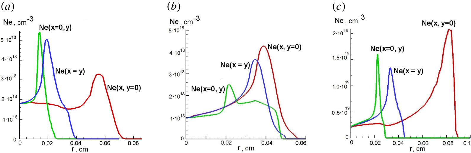
Degrees of electron density distribution asymmetry at  $t=15$ ns for the cases
 $A$ (
 $\unicode[STIX]{x1D6FD}=5.2^{\circ }$;
 $\unicode[STIX]{x1D70F}=2$ ns) (a),
 $C$ (
 $\unicode[STIX]{x1D6FD}=45^{\circ }$,
 $\unicode[STIX]{x1D70F}=2$ ns) (b) and
 $D$ (
 $\unicode[STIX]{x1D6FD}=21^{\circ }$;
 $\unicode[STIX]{x1D70F}=10$ ns) (c). The green lines correspond to the 1-D distributions along the lines
 $x=0$, the red lines do along the lines
 $y=0$ and the blue lines along the lines
 $x=y$.
 $r=\sqrt{x^{2}+y^{2}}$.

Figure 13(c) shows three 1-D electron density distributions along the rays  $(0,y>0)$,
 $(x>0,0)$ and
 $(x>0,y=x)$ at
 $t=15$ ns. These demonstrate more clearly than figure 10 the degree of symmetry of the electron density depression at the centre. The azimuthal symmetry of the electron density hole plays an important role for the possibility of high quality transportation of high intensity laser pulses in the waveguide, formed by the plasma channel. Figure 13 demonstrates that the sharpness of the electron density minimum for the case
 $D$ in the
 $x$-direction is approximately 2–3 times lower than in the
 $y$-direction at distances
 $r<150~\unicode[STIX]{x03BC}\text{m}$ from the centre of the plasma channel.
In § 3.2.2 we presented the results of the simulation of the case  $B$ for a considerably shorter laser pulse with duration
 $\unicode[STIX]{x1D70F}=2$ ns, keeping the laser energy,
 $J_{\text{tot}}$, the same. The case
 $B$ has a similar focusing angle. It is
 $26^{\circ }$ instead of
 $21^{\circ }$ for the case
 $D$. We may conclude that the difference in laser pulse duration (5 times) is much more important than the difference in the focusing angle (
 ${\sim}20\,\%$), so that almost all the difference in the symmetry of the plasma channel in these two simulations may be ascribed to the influence of the laser pulse duration. We see that in the case
 $B$ the plasma channel at
 $t=15$ ns is much more symmetric than in the case
 $D$. We may conclude that shorter laser pulses generate more symmetric channels in plasma.
3.4 Angular asymmetry of electron density distribution
We considered the evolution of the electron density distribution for the case  $B$ (
 $\unicode[STIX]{x1D6FD}=26^{\circ }$;
 $\unicode[STIX]{x1D70F}=2$ ns) in the relevant vicinity of the plasma channel axis in § 3.2.2 (see figure 8). We showed that the angular asymmetry changes its sign in the time interval,
 $10~\text{ns}<t<15~\text{ns}$. Hence, the most symmetric distribution of plasma density in the
 $(x,y)$ plane takes place during this interval. A similar situation takes place for the case
 $C$ with wider angle
 $\unicode[STIX]{x1D6FD}$ and the same pulse duration,
 $\unicode[STIX]{x1D70F}$. The degree of the asymmetry at
 $t=15$ ns can be seen in figure 13(b). It can be compared with figure 8(c). In both of these cases there is sufficient time for symmetrization after the laser pulse, which introduces asymmetry, and before the detaching of the shock wave from the hot plasma bubble, when homogeneous ambient gas and high thermal conduction in the bubble mitigate the asymmetry.
For small  $\unicode[STIX]{x1D6FD}$ (see case
 $A$), the initial asymmetry, introduced by the laser, is so high that it is not decreased considerably by the moment of the shock wave detaching. The electron density asymmetry at
 $t=15$ ns for the case
 $A$ is shown in figure 13(a). When the laser pulse is long (case
 $D$), then there is not enough time to mitigate the asymmetry, which is being introduced continuously during the laser pulse propagation. As a result the asymmetry remains very high up to
 $t=15$ ns, when the mitigation effect begins to decline (see figure 13c).
Thus, we conclude that the sufficiently large focusing angle  $\unicode[STIX]{x1D6FD}\sim 25^{\circ }{-}45^{\circ }$ of the laser beam and a duration of the order of
 $\unicode[STIX]{x1D70F}\sim 2$ ns need to be utilized to obtain an azimuthally symmetric plasma channel after approximately 10 ns after the laser pulse. Here, we used the parameters of the laser beam and plasma specified in § 3.1. We note that the above mentioned focusing angle and laser duration can depend on other parameters of the laser beam and the initial pressure of the neutral gas.
4 Conclusions
The solution of the Maxwell equations allows us to describe the electromagnetic field distribution and the electromagnetic radiation energy deposition in the focus region. The detailed simulations were performed using a modification of the MHD code MARPLE with the goal of investigating the process of the channel symmetrization, when the asymmetry of the initial channel is imprinted by the asymmetric deposition of the laser energy. The dissipative 2-D MHD simulations reveal a rather complicated structure of the plasma dynamics. Nevertheless, the simulations show a way to reach regimes of symmetric plasma channel formation.
We performed simulations for different focusing angles  $\unicode[STIX]{x1D6FD}$ and durations
 $\unicode[STIX]{x1D70F}$ of the laser pulse. The simulation, corresponding to
 $\unicode[STIX]{x1D6FD}=5.2^{\circ }$ and
 $\unicode[STIX]{x1D70F}=2$ ns, shows that the plasma channel is highly asymmetric. In order to find a way towards azimuthally symmetric channel formation, we performed two 2-D simulation runs with
 $\unicode[STIX]{x1D6FD}=26^{\circ }$ and
 $\unicode[STIX]{x1D6FD}=45^{\circ }$ for the laser pulse duration
 $\unicode[STIX]{x1D70F}=2$ ns. The simulations show that approximately azimuthally symmetric plasma channels in the close vicinity of the axis are formed approximately
 $\unicode[STIX]{x0394}t\sim 10$ ns after the laser pulse power peak reaches the focus. We performed also simulation with longer laser pulse durations,
 $\unicode[STIX]{x1D70F}=10$ ns, and
 $\unicode[STIX]{x1D6FD}=21^{\circ }$. The asymmetry introduced by the laser energy deposition is enhanced in this case. As a result, the plasma channel formed under these conditions is not suitable for guiding of high intensity laser pulses. We conclude that, by optimizing the laser–target parameters (duration of laser pulse
 $\unicode[STIX]{x1D70F}$, its energy, time delay
 $\unicode[STIX]{x0394}t$ and focusing angle of the laser pulse
 $\unicode[STIX]{x1D6FD}$), it is possible to find an optimal set of parameters for the formation of the plasma waveguide channel structure.
We also studied the possible symmetrization of the plasma channel due to the late stage expansion of the hot plasma. The simulations show that the hot plasma bubble at the moment of its formation is not azimuthally symmetric. At this moment the shock wave detaches from the hot bubble, which becomes almost isobaric. The further evolution of the remaining bubble is governed mainly by the thermal conduction and by the vortex motion. The vortices are excited just before the shock wave detachment. We see that the most symmetric channel is formed at approximately  $t=10{-}15$ ns for the case where the focusing angle is
 $\unicode[STIX]{x1D6FD}=26^{\circ }$ and the laser pulse duration is
 $\unicode[STIX]{x1D70F}=2$ ns. Then, the asymmetry starts to grow due to the vortex motion. A similar problem was studied by Kurzweil et al. (Reference Kurzweil, Livne and Meerson2003), where it was shown that the vortex motion leads to a strong mixing of the hot bubble with the ambient gas and to the complete loss of symmetry. When the shock wave is not yet detached from the hot bubble, the homogeneous ambient gas effects can lead to a symmetrization. So the most symmetric state of the hot bubble may occur right before the shock wave runs away.
Acknowledgements
We are very grateful to M. Basko, B. Meerson and I. Tsygvintsev for valuable advice. This work was supported by the project High Field Initiative (CZ.02.1.01/0.0/ 0.0/15003/0000449) from European Regional Development Fund, by grant MEYS CR CZ.02.2.69/0.0/0.0/16_027/0008465, MEYS CR LTT17015 (Research in the frame of International center of dense magnetized plasma), MEYS CR CZ.02.1.01/0.0/0.0/16-019/0000778 (Center of advanced applied sciences), and US DOE Office of Science, Offices of HEP and FES, under Contract No. DE-AC02-05CH11231. This work was also supported by the Ministry of Education, Youth, and Sports of the Czech Republic (Programmes NPU I Project No. LO1602, and Large Research Infrastructure Project No. LM2015086). The research is carried out using the equipment of the shared research facilities of HPC computing resources at Lomonosov Moscow State University and supercomputers at Joint Supercomputer Center of the Russian Academy of Sciences (JSCC RAS).
Appendix A. Derivation of the expression (2.2) for spatial distribution of electric field in knife-like focus of the laser beam
In order to solve (2.1) we introduce elliptic cylindrical coordinates,  $\unicode[STIX]{x1D70E}$ and
 $\unicode[STIX]{x1D70F}$ (Korn & Korn Reference Korn and Korn1968)
 $$\begin{eqnarray}\displaystyle & \displaystyle \frac{y^{2}}{a^{2}\unicode[STIX]{x1D70E}^{2}}+\frac{x^{2}}{a^{2}(\unicode[STIX]{x1D70E}^{2}-1)}=1, & \displaystyle\end{eqnarray}$$
 $$\begin{eqnarray}\displaystyle & \displaystyle \frac{y^{2}}{a^{2}\unicode[STIX]{x1D70F}^{2}}+\frac{x^{2}}{a^{2}(\unicode[STIX]{x1D70F}^{2}-1)}=1. & \displaystyle\end{eqnarray}$$
It follows from these expressions that
 $$\begin{eqnarray}y=a\unicode[STIX]{x1D70E}\unicode[STIX]{x1D70F},\quad x^{2}=a^{2}(\unicode[STIX]{x1D70E}^{2}-1)(1-\unicode[STIX]{x1D70F}^{2}),\end{eqnarray}$$
where  $\unicode[STIX]{x1D70E}\geqslant 1$,
 $-1\leqslant \unicode[STIX]{x1D70F}\leqslant 1$ and
 $a$ is a positive constant value, which is determined below. In the elliptic cylindrical coordinates, equation (2.1) takes the following form (Korn & Korn Reference Korn and Korn1968):
 $$\begin{eqnarray}\sqrt{\unicode[STIX]{x1D70E}^{2}-1}\,\unicode[STIX]{x2202}_{\unicode[STIX]{x1D70E}}(\sqrt{\unicode[STIX]{x1D70E}^{2}-1}\,\unicode[STIX]{x2202}_{\unicode[STIX]{x1D70E}}E)+\sqrt{1-\unicode[STIX]{x1D70F}^{2}}\,\unicode[STIX]{x2202}_{\unicode[STIX]{x1D70F}}(\sqrt{1-\unicode[STIX]{x1D70F}^{2}}\,\unicode[STIX]{x2202}_{\unicode[STIX]{x1D70F}}E)=k^{2}a^{2}(\unicode[STIX]{x1D70F}^{2}-\unicode[STIX]{x1D70E}^{2})E.\end{eqnarray}$$
We search for the solution of (A 4) in the form  $E(\unicode[STIX]{x1D70E},\unicode[STIX]{x1D70F})=\unicode[STIX]{x1D6F4}(\unicode[STIX]{x1D70E})T(\unicode[STIX]{x1D70F})$. Substituting this expression into (A 4) we obtain a system of ordinary differential equations for functions
 $\unicode[STIX]{x1D6F4}$ and
 $T$
 $$\begin{eqnarray}\displaystyle & \displaystyle \sqrt{\unicode[STIX]{x1D70E}^{2}-1}\,\frac{\text{d}}{\text{d}\unicode[STIX]{x1D70E}}\left(\sqrt{\unicode[STIX]{x1D70E}^{2}-1}\,\frac{\text{d}\unicode[STIX]{x1D6F4}}{\text{d}\unicode[STIX]{x1D70E}}\right)=(\unicode[STIX]{x1D6EC}-k^{2}a^{2}\unicode[STIX]{x1D70E}^{2})\unicode[STIX]{x1D6F4}, & \displaystyle\end{eqnarray}$$
 $$\begin{eqnarray}\displaystyle & \displaystyle \sqrt{1-\unicode[STIX]{x1D70F}^{2}}\,\frac{\text{d}}{\text{d}\unicode[STIX]{x1D70F}}\left(\sqrt{1-\unicode[STIX]{x1D70F}^{2}}\,\frac{\text{d}T}{\text{d}\unicode[STIX]{x1D70F}}\right)=-(\unicode[STIX]{x1D6EC}-k^{2}a^{2}\unicode[STIX]{x1D70F}^{2})T. & \displaystyle\end{eqnarray}$$
The solution of these equations can be expressed in terms of Mathieu functions (Olver et al. Reference Olver, Lozier, Boisvert and Clark2010).
First, we consider the limiting case of  $ka\gg 1$. Here, the solution,
 $T(\unicode[STIX]{x1D70F})$, differs from zero only at a small value of
 $|\unicode[STIX]{x1D70F}|$. Using
 $|\unicode[STIX]{x1D70F}|\ll 1$, while
 $ka\unicode[STIX]{x1D70F}^{2}$ may be
 ${\sim}O(1)$, we rewrite (A 6) in the following form:
 $$\begin{eqnarray}\frac{\text{d}^{2}T}{\text{d}\unicode[STIX]{x1D70F}^{2}}+(\unicode[STIX]{x1D6EC}-k^{2}a^{2}\unicode[STIX]{x1D70F}^{2})T=0\,.\end{eqnarray}$$
This equation has a set of localized solutions that are actually solutions of an eigenvalue problem, with  $\unicode[STIX]{x1D6EC}$ being the eigenvalue. They can be expressed in terms of Hermite polynomials and exponents (Olver et al. Reference Olver, Lozier, Boisvert and Clark2010). These solutions have nodes with the exception of one solution. The only eigenfunction without any node corresponds to the Gaussian beam, lowest, prime eigensolution and the lowest eigenvalue
 $\unicode[STIX]{x1D6EC}$
 $$\begin{eqnarray}T\propto \exp (-ka\unicode[STIX]{x1D70F}^{2}/2),\end{eqnarray}$$
with  $\unicode[STIX]{x1D6EC}=ka$, and
 $ka\gg 1$. If
 $ka\gg 1$, then equation (A 5) for the function
 $\unicode[STIX]{x1D6F4}$ takes the form
 $$\begin{eqnarray}\sqrt{\unicode[STIX]{x1D70E}^{2}-1}\,\frac{\text{d}}{\text{d}\unicode[STIX]{x1D70E}}\left(\sqrt{\unicode[STIX]{x1D70E}^{2}-1}\,\frac{\text{d}\unicode[STIX]{x1D6F4}}{\text{d}\unicode[STIX]{x1D70E}}\right)=(ka-k^{2}a^{2}\unicode[STIX]{x1D70E}^{2})\unicode[STIX]{x1D6F4}.\end{eqnarray}$$
When  $ka\gg 1$, it can be solved within the framework of the WKB approximation, i.e.
 $$\begin{eqnarray}\unicode[STIX]{x1D6F4}=b\exp (\text{i}S),\end{eqnarray}$$
where  $S$ and
 $|\text{d}S/\text{d}\unicode[STIX]{x1D70E}|$ are functions of
 $\unicode[STIX]{x1D70E}$, much larger than 1, whereas
 $b$ is a smoothly varying pre-exponent. In this case, the typical scale of the fast oscillating exponent
 $\exp (\text{i}S)$ is much less than the typical scale of the pre-exponent
 $b$ variations. It is easy to obtain the equation for
 $S$ as a function of variable
 $\unicode[STIX]{x1D70E}$. It can be written in the form
 $$\begin{eqnarray}\left(\frac{\text{d}S}{\text{d}\unicode[STIX]{x1D70E}}\right)^{2}=k^{2}a^{2}\frac{\unicode[STIX]{x1D70E}^{2}}{\unicode[STIX]{x1D70E}^{2}-1}.\end{eqnarray}$$
It yields
 $$\begin{eqnarray}S=ka\sqrt{\unicode[STIX]{x1D70E}^{2}-1}\text{sgn}(x).\end{eqnarray}$$
The pre-exponent  $b$ satisfies the equation
 $$\begin{eqnarray}(2S^{\prime }b^{\prime }+S^{\prime \prime }b)(\unicode[STIX]{x1D70E}^{2}-1)+S^{\prime }b\,\unicode[STIX]{x1D70E}=-\text{i}kab,\end{eqnarray}$$
where the prime denotes differentiation with respect to the variable  $\unicode[STIX]{x1D70E}$. Assuming that the solution of this linear ordinary differential equation of the first order has the form
 $b=|b|\exp (\text{i}\unicode[STIX]{x1D719})$, we obtain the following expressions for the amplitude
 $|b|$ and phase
 $\unicode[STIX]{x1D719}$:
 $$\begin{eqnarray}|b|\propto \frac{1}{\sqrt{\unicode[STIX]{x1D70E}}},\quad \unicode[STIX]{x1D719}=\frac{\text{sgn}(x)}{2}\arctan \left(\frac{1}{\sqrt{\unicode[STIX]{x1D70E}^{2}-1}}\right).\end{eqnarray}$$
Substituting expressions for  $\unicode[STIX]{x1D6F4}$ and
 $T$ in the formula for the single non-vanishing component of the electric field
 $E_{z}=E(x,y)\text{e}^{-\text{i}\unicode[STIX]{x1D714}t}=\unicode[STIX]{x1D6F4}(\unicode[STIX]{x1D70E})T(\unicode[STIX]{x1D70F})\text{e}^{-\text{i}\unicode[STIX]{x1D714}t}$, and taking into account (A 3) with
 $|\unicode[STIX]{x1D70F}|\ll 1$, we obtain an expression for stationary travelling electric field. Square of its absolute value is given by
 $$\begin{eqnarray}|E_{z}|^{2}\propto \frac{1}{\sqrt{x^{2}+a^{2}}}\exp \left(-ka\frac{y^{2}}{x^{2}+a^{2}}\right).\end{eqnarray}$$
It is useful to introduce a dimensionless parameter  $\unicode[STIX]{x1D6FC}$, which determines the angle of focusing of the laser pulse (see below) and the aspect ratio of energy distribution of electromagnetic energy in the plane
 $(x,y)$,
 $\unicode[STIX]{x1D6FC}=1/\sqrt{ka}$, when
 $ka\gg 1$. Substituting this relationship into (A 15), we obtain that the square of absolute value of the electric field
 $E$ depends on the coordinates
 $x$ and
 $y$ as
 $$\begin{eqnarray}|E|^{2}\propto \frac{1}{\sqrt{\unicode[STIX]{x1D6FC}^{4}k^{2}x^{2}+1}}\exp \left(-\frac{\unicode[STIX]{x1D6FC}^{2}k^{2}y^{2}}{\unicode[STIX]{x1D6FC}^{4}k^{2}x^{2}+1}\right).\end{eqnarray}$$
In the paraxial approximation the, averaged over the period of the electro-magnetic field, Poynting vector value is
 $$\begin{eqnarray}F=c\frac{\left\langle \left(\boldsymbol{E}\times \boldsymbol{B}\right)_{x}\right\rangle }{4\unicode[STIX]{x03C0}}=c\frac{|E|^{2}}{8\unicode[STIX]{x03C0}}.\end{eqnarray}$$
Combining (A 16) and (A 17), we obtain (2.2).
Note that we used the WKB approximation only to derive the distribution (A 16) of the electromagnetic energy in the focus along the beam axis, whereas the transverse distribution in the waist of the focus is determined by the diffraction effect. Equation (A 16) says that the longitudinal depth of the focus  $\unicode[STIX]{x1D706}\unicode[STIX]{x1D6FC}^{-2}/2\unicode[STIX]{x03C0}$ is approximately
 ${\sim}\unicode[STIX]{x1D6FC}^{-2}/2\unicode[STIX]{x03C0}$ times larger than the laser wavelength. It justifies the application of the WKB approximation for describing the longitudinal structure, when
 $\unicode[STIX]{x1D6FC}\ll 1$.
We analysed above the case of the TE polarization of an electromagnetic wave. However, if the parameter  $\unicode[STIX]{x1D6FC}$ is small, i.e.
 $\unicode[STIX]{x1D6FC}\ll 1$, the
 $|E|^{2}$ distribution does not depend on the polarization of the electromagnetic wave in the leading order. This fact can be explained by the the substitution
 $B_{z}\leftrightarrow E_{z}$ in (2.1) and (A 4), and by the fact that both the electric and magnetic fields in the wave are almost perpendicular to the
 $x$-axis, when
 $\unicode[STIX]{x1D6FC}\ll 1$.
Using our equations (A 8), (A 10), (A 12) and (A 14), and the symmetry TE $\,\leftrightarrow \,$TM, mentioned above, we write for small
 $\unicode[STIX]{x1D6FC}$ that
 $$\begin{eqnarray}|\boldsymbol{E}|^{2}|_{TM}=|\boldsymbol{B}|^{2}|_{TE}\approx |E|^{2}(x,y)|_{TE}\,\left(1+\frac{\unicode[STIX]{x1D6FC}^{4}k^{2}y^{2}}{(1+\unicode[STIX]{x1D6FC}^{4}k^{2}x^{2})^{2}}\right).\end{eqnarray}$$
We estimate that TM-polarization provides at  $\unicode[STIX]{x1D6FC}=1/2$ approximately 10 % higher energy deposition into plasma in the vicinity of the waist of the laser beam under the same conditions as the TE-polarization. For
 $\unicode[STIX]{x1D6FC}=1/4$ this value becomes approximately 3 %.
We note that the result (2.2) can be obtained, within the framework of the paraxial approximation for the Helmholtz wave equation. Both types of polarization are described by the same expression in this approximation. The Gaussian beams are well-known solutions of this equation (see, for example, Svetlo (Reference Svelto2010)). Using this approach for the case of a knife-like electromagnetic beam, one can obtain the spatial distribution of the laser energy flux  $F$.
We derived (A 16) assuming  $\unicode[STIX]{x1D6FC}\ll 1$. However, the values of
 $\unicode[STIX]{x1D6FC}$ up to
 $\unicode[STIX]{x1D6FC}=1/2$ (or
 $ka=4$) were used along with (2.2) in simulations. In order to determine what kind of error is introduced by this, we use the exact equations (A 5) and (A 6). The solution should be smooth in the whole space
 $(x,y)$. Then we would obtain
 $T\propto \text{ce}_{0}(\unicode[STIX]{x1D701},4)$, where
 $\unicode[STIX]{x1D701}=\arccos (\unicode[STIX]{x1D70F})$ and
 $\unicode[STIX]{x1D6F4}\propto \text{ce}_{0}(\text{i}u,4)$, and where
 $u=\text{arccosh}\,(\unicode[STIX]{x1D70E})$. Here,
 $\text{ce}_{0}(\cdot ,\cdot )$ is one of standard Mathieu functions (Olver et al. Reference Olver, Lozier, Boisvert and Clark2010). This solution represents a standing wave. However, our goal is to find a solution, which would behave as
 $\propto \exp (\text{i}kr)/\sqrt{r}$ at
 $r=\sqrt{x^{2}+y^{2}}\rightarrow \infty$ at the half-plane
 $x>0$. This condition corresponds to a pure travelling wave in this region and introduces some
 $x\rightarrow -x$ asymmetry. In this case, we are forced to set a boundary condition at some place outside the beam so that the solution will be in the simple form,
 $E=T(\unicode[STIX]{x1D70F})\,\unicode[STIX]{x1D6F4}(\unicode[STIX]{x1D70E})$. We set that
 $E=0$ at
 $x=0$, when
 $|y|\geqslant a$. Then
 $$\begin{eqnarray}T\propto \text{se}_{1}(\unicode[STIX]{x1D701},4),\end{eqnarray}$$
where the Mathieu function  $\text{se}_{1}(\unicode[STIX]{x1D701},q)$ is defined in the handbook by Olver et al. (Reference Olver, Lozier, Boisvert and Clark2010), and
 $\unicode[STIX]{x1D6F4}(\unicode[STIX]{x1D70E}(x,0))$ is obtained from a numerical solution of the equation
 $$\begin{eqnarray}\left(\unicode[STIX]{x1D712}^{2}+1\right)\unicode[STIX]{x1D6F4}_{\unicode[STIX]{x1D712}\unicode[STIX]{x1D712}}+\unicode[STIX]{x1D712}\unicode[STIX]{x1D6F4}_{\unicode[STIX]{x1D712}}+\left(4q\unicode[STIX]{x1D712}^{2}+2q-a_{0}(q)\right)\unicode[STIX]{x1D6F4}=0,\end{eqnarray}$$
with the boundary condition
 $$\begin{eqnarray}\unicode[STIX]{x1D6F4}\propto \exp (\text{i}ka\unicode[STIX]{x1D712})/\sqrt{\unicode[STIX]{x1D712}}+\cdots \quad \text{at }\unicode[STIX]{x1D712}\rightarrow +\infty .\end{eqnarray}$$
Here,  $\unicode[STIX]{x1D712}=x/a$,
 $q=k^{2}a^{2}/4$ and this equation is equivalent to (A 5). The boundary condition fixes the solution that corresponds to the outgoing travelling wave far from the focus at the half-plane
 $x>0$.
Distributions of  $|E|^{2}$ along the lines
 $x=0$ (a) and
 $y=0$ (b) at
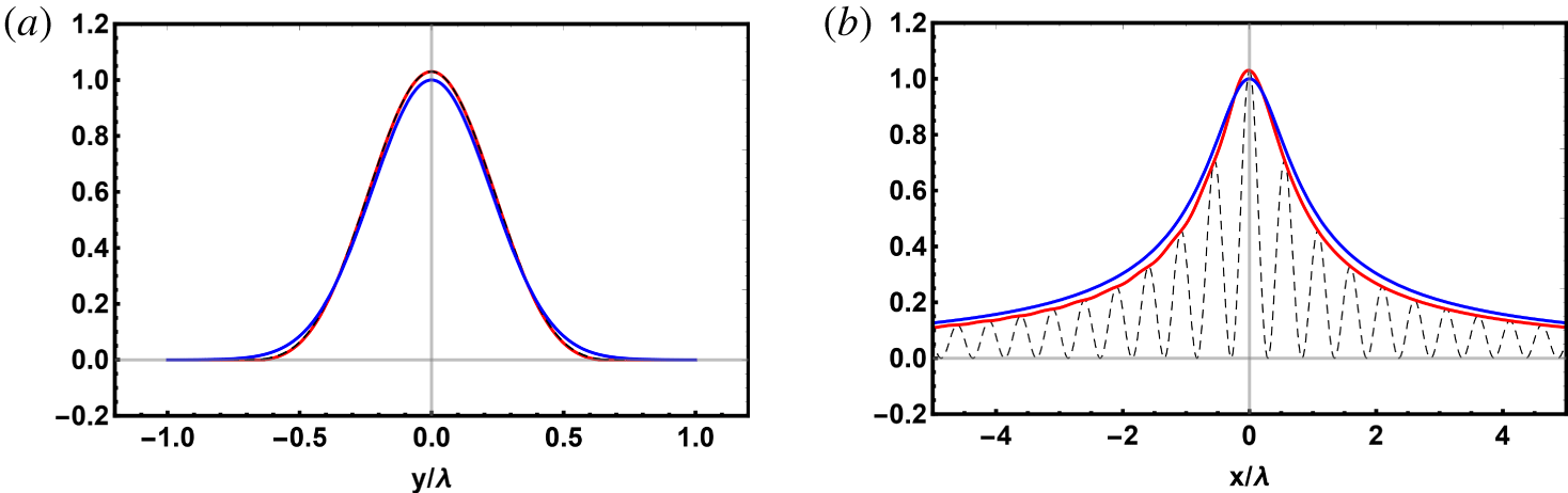
 $\unicode[STIX]{x1D6FC}=1/2$. The former presents the transverse distribution with respect to the direction of laser beam propagation, whereas the latter corresponds to the distribution along the beam. The blue lines present distributions (2.2), whereas the red ones correspond to solutions of the exact (A 7) and (A 10) with the same
 $\unicode[STIX]{x1D6FC}$ and total flux. The black dashed line presents half of the standing wave mentioned in the text. Note that the latter is almost indistinguishable from the red line in (a), although it is different.

Figure 14 shows the comparisons of two 1-D cross-sections of the  $|E|^{2}$ distribution obtained from the solution of both (2.2) and the exact equations (A 19)–(A 21). We used the same parameter
 $\unicode[STIX]{x1D6FC}=1/2$ and the same flux
 $J$, and normalize the plots to the maximum value from (2.2). For clarification, we plot also half of
 $|E|^{2}$ for standing wave solution, described in the previous paragraph. It is interesting that, although the travelling wave solution and the standing one are surely different, nevertheless, the difference cannot be resolved in figure 14 for this parameter
 $\unicode[STIX]{x1D6FC}=1/2$. We may mention another manifestation of the same feature at
 $\unicode[STIX]{x1D6FC}=1/2$: the intensity of the reflected wave in the region
 $x<0$,
 $r\rightarrow \infty$ is only approximately
 $10^{-4}$ of the incoming travelling wave. In summary, we conclude that the inaccuracy of (2.2) is less than
 ${\sim}3\,\%$–4 % of the maximum value even for our highest value of
 $\unicode[STIX]{x1D6FC}=1/2$. For lower
 $\unicode[STIX]{x1D6FC}\lesssim 1/\sqrt{8}\approx 0.35$ the difference becomes negligible.
Appendix B. Physical model implemented by the code MARPLE
The code MARPLE implements the following system of MHD equations:
 $$\begin{eqnarray}\displaystyle & \displaystyle \unicode[STIX]{x2202}_{t}\unicode[STIX]{x1D70C}+\unicode[STIX]{x1D735}\boldsymbol{\cdot }\unicode[STIX]{x1D70C}\boldsymbol{v}=0; & \displaystyle\end{eqnarray}$$
 $$\begin{eqnarray}\displaystyle & \displaystyle \unicode[STIX]{x1D70C}\left(\unicode[STIX]{x2202}_{t}\boldsymbol{v}+\left(\boldsymbol{v}\boldsymbol{\cdot }\unicode[STIX]{x1D735}\right)\boldsymbol{v}\right)=-\unicode[STIX]{x1D735}p-\frac{1}{c}~\boldsymbol{j}\times \boldsymbol{B}; & \displaystyle\end{eqnarray}$$
 $$\begin{eqnarray}\displaystyle & \displaystyle \unicode[STIX]{x1D735}\times \boldsymbol{B}=\frac{4\unicode[STIX]{x03C0}}{c}~\boldsymbol{j};\quad \boldsymbol{j}=\unicode[STIX]{x1D70E}\left(\boldsymbol{E}+\frac{1}{c}\boldsymbol{v}\times \boldsymbol{B}\right); & \displaystyle\end{eqnarray}$$
 $$\begin{eqnarray}\displaystyle & \displaystyle \unicode[STIX]{x2202}_{t}\boldsymbol{B}=-c\unicode[STIX]{x1D735}\times \boldsymbol{E};\quad \unicode[STIX]{x1D735}\boldsymbol{\cdot }\boldsymbol{B}=0; & \displaystyle\end{eqnarray}$$
 $$\begin{eqnarray}\displaystyle & \displaystyle \unicode[STIX]{x1D70C}\left(\unicode[STIX]{x2202}_{t}\unicode[STIX]{x1D700}_{e}+\boldsymbol{v}\boldsymbol{\cdot }\unicode[STIX]{x1D735}\unicode[STIX]{x1D700}_{e}\right)+p_{e}\unicode[STIX]{x1D735}\boldsymbol{\cdot }\boldsymbol{v}=\unicode[STIX]{x1D735}\boldsymbol{\cdot }(\unicode[STIX]{x1D705}_{e}\unicode[STIX]{x1D735}T_{e})+\frac{\boldsymbol{j}^{2}}{\unicode[STIX]{x1D70E}}-Q_{ie}+Q; & \displaystyle\end{eqnarray}$$
 $$\begin{eqnarray}\displaystyle & \displaystyle \unicode[STIX]{x1D70C}\left(\unicode[STIX]{x2202}_{t}\unicode[STIX]{x1D700}_{i}+\boldsymbol{v}\boldsymbol{\cdot }\unicode[STIX]{x1D735}\unicode[STIX]{x1D700}_{i}\right)+p_{e}\unicode[STIX]{x1D735}\boldsymbol{\cdot }\boldsymbol{v}=\unicode[STIX]{x1D735}\boldsymbol{\cdot }(\unicode[STIX]{x1D705}_{i}\unicode[STIX]{x1D735}T_{i})+Q_{ie}. & \displaystyle\end{eqnarray}$$
Besides quite standard notations for plasma density, its velocity, electric current and electric and magnetic fields, we use here less common notations. Here,  $p=p_{e}+p_{i}$ is the plasma pressure determined by the sum of the pressures of the electron,
 $p_{e}$, and ion components,
 $p_{i}$;
 $\unicode[STIX]{x1D700}_{e}$ and
 $\unicode[STIX]{x1D700}_{i}$ are specific internal energies of the electron and ion components of the plasma, respectively;
 $\unicode[STIX]{x1D70E}$ is the electric conductivity of the plasma;
 $\unicode[STIX]{x1D705}_{e}$ and
 $\unicode[STIX]{x1D705}_{i}$ are coefficients of thermal conduction in the electron and ion components of the plasma;
 $T_{e}$ and
 $T_{i}$ are temperatures of the electron and ion components the of plasma;
 $Q_{ie}$ represents the energy exchange between the electron and ion components; and
 $Q$ is the rate of energy deposition from the laser beam to plasma per unit volume and per unit time. The latter value is defined in § 2.
Equations (B 1) and (B 2) are the continuity equation and Newton’s second law, respectively. Equations (B 3)–(B 4) give three out of four Maxwell equations (in the quasi-stationary approximation) and Ohm’s law. The remaining Maxwell equation,  $\unicode[STIX]{x1D735}\boldsymbol{\cdot }\boldsymbol{E}=4\unicode[STIX]{x03C0}q$, where
 $q$ is the volume density of the total electric charge, is reduced to
 $q=0$ for macroscopic plasma volumes. The latter condition is usually referred to as the condition of quasi-neutrality:
 $n_{e}=Zn_{i}$, where
 $Z$ is the mean charge of compound plasma component of heavy particles, consisting of ions and neutrals, and
 $n_{e}$ and
 $n_{i}$ are the concentrations of electrons and the heavy particles, respectively. We include neutrals in a joint component consisting of neutrals and ions in this section. This heavy particle component is referred to as ‘ions’ and is designated by the subscript
 $i$ here. The mean charge
 $Z$ is defined here from the Saha ionization equation. Equations (B 5) and (B 6) are heat equations for electron and ion components, respectively. The thermodynamic parameters of these components
 $\unicode[STIX]{x1D700}_{e,i}$ and
 $p_{e,i}$ actually correspond to an ideal gas, however,
 $\unicode[STIX]{x1D700}_{e}$ includes the energy of ionization. Quite similar model for description of partially ionized hydrogen plasma was described by Bobrova et al. (Reference Bobrova, Esaulov, Sakai, Sasorov, Spence, Butler, Hooker and Bulanov2002).
Equations (B 1)–(B 6) are written here in a simplified form, which is relevant to the present problem. Nevertheless, the full MHD model implemented in the code MARPLE includes: plasma viscosity, anisotropic (tensor) structures of  $\unicode[STIX]{x1D70E}$ and
 $\unicode[STIX]{x1D705}_{e,i}$, thermal radiation transport etc. The kinetic coefficients
 $\unicode[STIX]{x1D70E}$,
 $\unicode[STIX]{x1D705}_{e,i}$, as well as
 $Q_{ie}$ were calculated using the model by Braginskii (Reference Braginskii and Leontovich1963). The model was extended to take into account collisions with neutrals analogously to Bobrova et al. (Reference Bobrova, Esaulov, Sakai, Sasorov, Spence, Butler, Hooker and Bulanov2002).
The code MARPLE utilizes different types of boundary conditions. See for example Bagdasarov et al. (Reference Bagdasarov, Sasorov, Gasilov, Boldarev, Olkhovskaya, Benedetti, Bulanov, Gonsalves, Mao and Schroeder2017a). They may include connection to an external low frequency electromagnetic generator. However, we do not include such external generators in the present problem. Moreover, we chose a sufficiently large size of the simulation domain so that the disturbances in the initially homogeneous cold gas do not reach its boundaries. As a result, the exact form of passive conditions for plasma parameters at the boundaries does not play any role in the present problem.
Magnetic field in the initial state is assumed negligible. The simple form of Ohms law, presented in (B 3), and the initial condition lead to the magnetic field  $\boldsymbol{B}$ being equal to 0 during the whole simulation. We estimated that the battery effect, neglected in (B 3), and caused by non-vanishing
 $\unicode[STIX]{x1D735}p_{e}\times \unicode[STIX]{x1D735}T_{e}$, leads to the generation of a magnetic field that could be neglected for the present problem. Our model contains, however, the effect
 $\unicode[STIX]{x1D735}p\times \unicode[STIX]{x1D735}\unicode[STIX]{x1D70C}$ in the equation of motion (B 2). It is similar to some extent to the battery effect and leads to the generation of vorticity in the hot plasma bubble. This effect plays an important role for our problem and is considered above.
The physical model, presented here, as well as the code MARPLE as a whole were used for successful simulations of different experiments, as it was mentioned above.