1. Introduction
In statistics, there are two main paradigms: classical and Bayesian statistics. A notorious problem with the Bayesian approach is the choice of prior credences. Because of Bertrand-style paradoxes, there does not seem to be any privileged way of choosing them. Classical statistics is, in a sense, an attempt to factor them out. A problematic consequence of this approach is its limited applicability. Another problem is how to interpret classical notions (such as significance levels) in terms of degrees of evidential support (e.g., Lindley Reference Lindley1957; Berger and Sellke Reference Berger and Sellke1987; Casella and Berger Reference Casella and Berger1987). Setting these issues aside, the purpose of this article is rather to investigate the extent to which classicists and Bayesians can (in some suitable sense of the word) agree in situations in which classical statistics is applicable. More precisely: Is there always a nontrivial prior credence distribution such that, for any possible observation, a Bayesian with that credence will agree with the classicist whether the observation speaks in favor of rejecting the hypothesis? The answer, as we will see, is no. In sections 2 and 3, I present the classical and Bayesian frameworks, respectively. In section 4, I define what I take to be a reasonable notion of agreement, and construct a case in which agreement is impossible. In section 5, I present a more general diagnosis of the conflict between classical statistics and the Bayesian theory of rational degrees of belief.
2. Classical Statistics
In classical statistics, hypotheses about the distribution of various properties in a population are tested by observing random samples of it. On the assumption that the sample is random, the conditional probability
 for every possible observation E and hypothesis H is usually derived as a matter of combinatorics. Given a particular hypothesis H 0 (a so-called null hypothesis, which is the hypothesis to be tested), a rejection region for H 0 has to be selected, which is the set of outcomes leading to the rejection of H 0. Formally, if Ω is a nonempty set of possible outcomes (a sample space), Σ is a σ-algebra on Ω (an event space), and Θ is a nonempty set of hypotheses, there is a function
 such that, for each hypothesis
 , the function
 is a probability function. A rejection region for a hypothesis
 is an event
 such that H 0 is rejected just in case an event
 is observed such that
 . The question is, what should this region look like?
Saying, for instance, that one should reject a hypothesis whenever an observation is made whose probability given that hypothesis is below a certain threshold will not do, since it means rejecting the hypothesis that a coin is fair given any sufficiently long sequence of observed tosses. Likewise, it means rejecting the hypothesis that the length of the male population is somewhat normally distributed around an average of 1.85 meters, after having observed a sample with exactly that average (in general, it is highly unlikely for the average of the sample to exactly coincide with the average of the population). There are essentially two classical approaches to this problem, one by Fisher and the other by Neyman and Pearson. I will look at each of them in turn.
2.1. Fisher
Instead of rejecting a hypothesis H just in case an event E is observed such that
 is sufficiently low (which would be absurd), the general idea proposed by Fisher (Reference Fisher1925) is to reject H just in case P(E or something more extreme|H) is sufficiently low. Formally, for a given hypothesis H, let ≺H be a strict partial order on Ω such that, for any
 ,
 . The intended interpretation of
 is that y is more extreme than x with respect to H. For any event
 , the so-called p-value of E with respect to H and ≺H can then be defined as follows:

Thus, the p-value of E with respect to H and ≺H is to be understood as the probability of observing E or something more extreme under the assumption that H is true. The lower the p-value, the more reason one has to reject H, according to Fisher. For instance, consider again the null hypothesis that the length of the male population is normally distributed around an average of 1.85 meters. Assuming that the measured average of a sample is to be considered more extreme, the more it differs from 1.85, the p-value of measuring an average of exactly 1.85 meters is 1. Such a high p-value will not warrant the rejection of the null hypothesis.
But what makes an outcome more extreme than some other outcome with respect to given hypothesis H? In general, it would be unwise to simply stipulate that
 just in case
 . For one thing, it might be the case that
 , in which case the probabilities in question are undefined. Or it might be the case that
 for all
 . That typically happens when Ω is the set ℝ of real numbers, Σ is the set of Lebesgue measurable subsets of ℝ, and
 is defined as the integral of a continuous probability density function
 . But it is equally unwise to stipulate in such cases that
 just in case
 , as the following example illustrates.
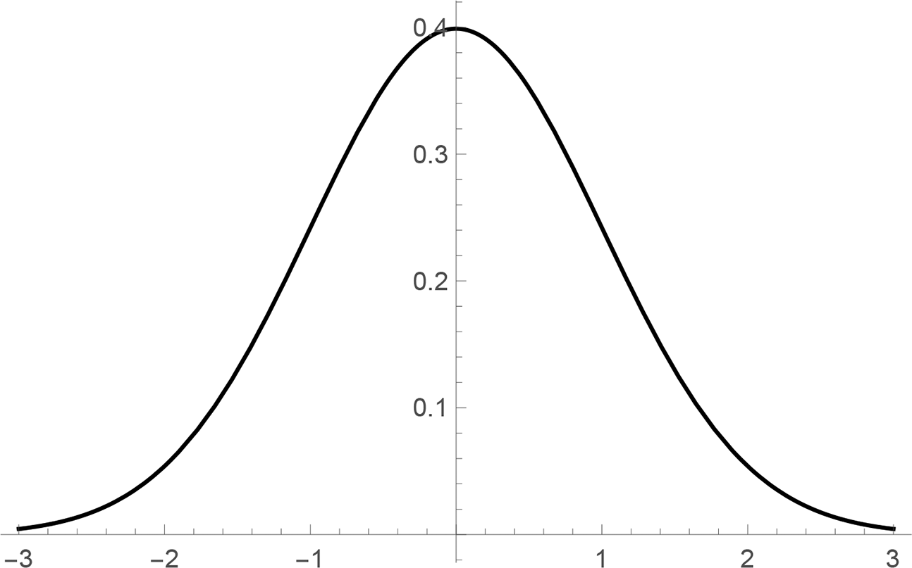
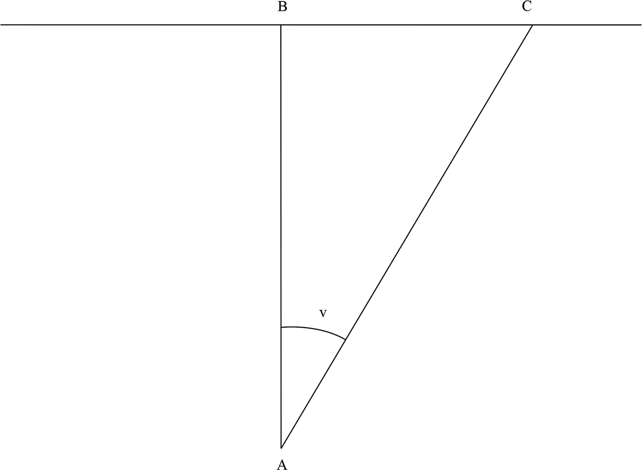
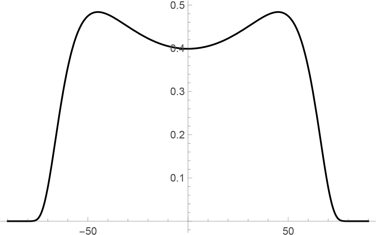
Example 1 (The shooting range). Suppose you want to test whether the aim on a rifle is straight (with respect to the horizontal direction). You go to a shooting range and fix the rifle aimed at a particular target. Your plan is to fire several bullets at the target, measure the horizontal distance in decimeters between the target and the point of impact for each bullet, and calculate the mean. Your null hypothesis H is that the aim is straight. Suppose that, on the assumption that the null hypothesis is true due to random influences (in particular the shape of the bullet leaving the pipe), the sampled mean can be expected to be normally distributed around 0 with variance 1, as depicted in figure 1. Any statistics textbook will tell you that an outcome y is to be considered more extreme than an outcome x relative to the null hypothesis just in case the absolute distance between y and the mean 0 is greater than the absolute difference between x and 0. In other words, for any
 ,
 just in case
 . One might be tempted to infer this from the shape of the probability density function f in figure 1 alone, since
 just in case
 . To see why that would be unwise, let us look at a different but equivalent representation of the same situation, depicted in figure 2. Let A be the point 1 decimeter from the target in the direction of the rifle, let B be the target, and let C be a point to the left or right of the target indicating the measured mean deviation, and consider the angle v between AB and AC, ranging in the open interval between −90 to 90 degrees. With the same random influences as before, the expected distribution on this angle is given by the probability density function g depicted in figure 3. But here it is no longer the case that, for any angles
 ,
 just in case
 .
Expected distribution on the measured mean according to the null hypothesis, given by a probability density function
 .

Measured mean represented by the angle
 .

Expected distribution on the angle corresponding to the measured mean according to the null hypothesis, given by a probability density function
 .

In conclusion, the relation of being a more extreme outcome with respect to a particular hypothesis cannot be inferred from the probability distribution associated with the hypothesis in any obvious way. Although it is intuitively clear enough in practice what relation to use, it does make Fisher’s theory less appealing from a philosophical point of view.
2.2. Neyman and Pearson
A philosophically more sophisticated theory is offered by Neyman and Pearson (Reference Neyman and Pearson1933a, Reference Neyman and Pearson1933b). The basic intuition is that, whether a hypothesis should be rejected depends on whether there are better alternatives, that is, whether there are plausible enough alternative hypotheses according to which the probability of the observation is higher. More specifically, determining an adequate rejection region for the null hypothesis involves two notions: type 1 and type 2 errors. To commit a type 1 error is to reject a true null hypothesis. To commit a type 2 error is to not reject a false null hypothesis. Naturally, one does not want to reject a true null hypothesis. Hence, for each proposed rejection region
 , one may ask: What is the probability of rejecting the null hypothesis, on the assumption that it is true? The answer, of course, is
 . For some suitably small number
 (e.g.,
 ), it is therefore reasonable to require that
 . However, if all we care about is minimizing the risk of making a type 1 error, then we should let
 and never reject any null hypothesis. In general, however, even if we require that
 , this condition does not single out a unique rejection region. As illustrated by Barnett (Reference Barnett1999, 167–68), if
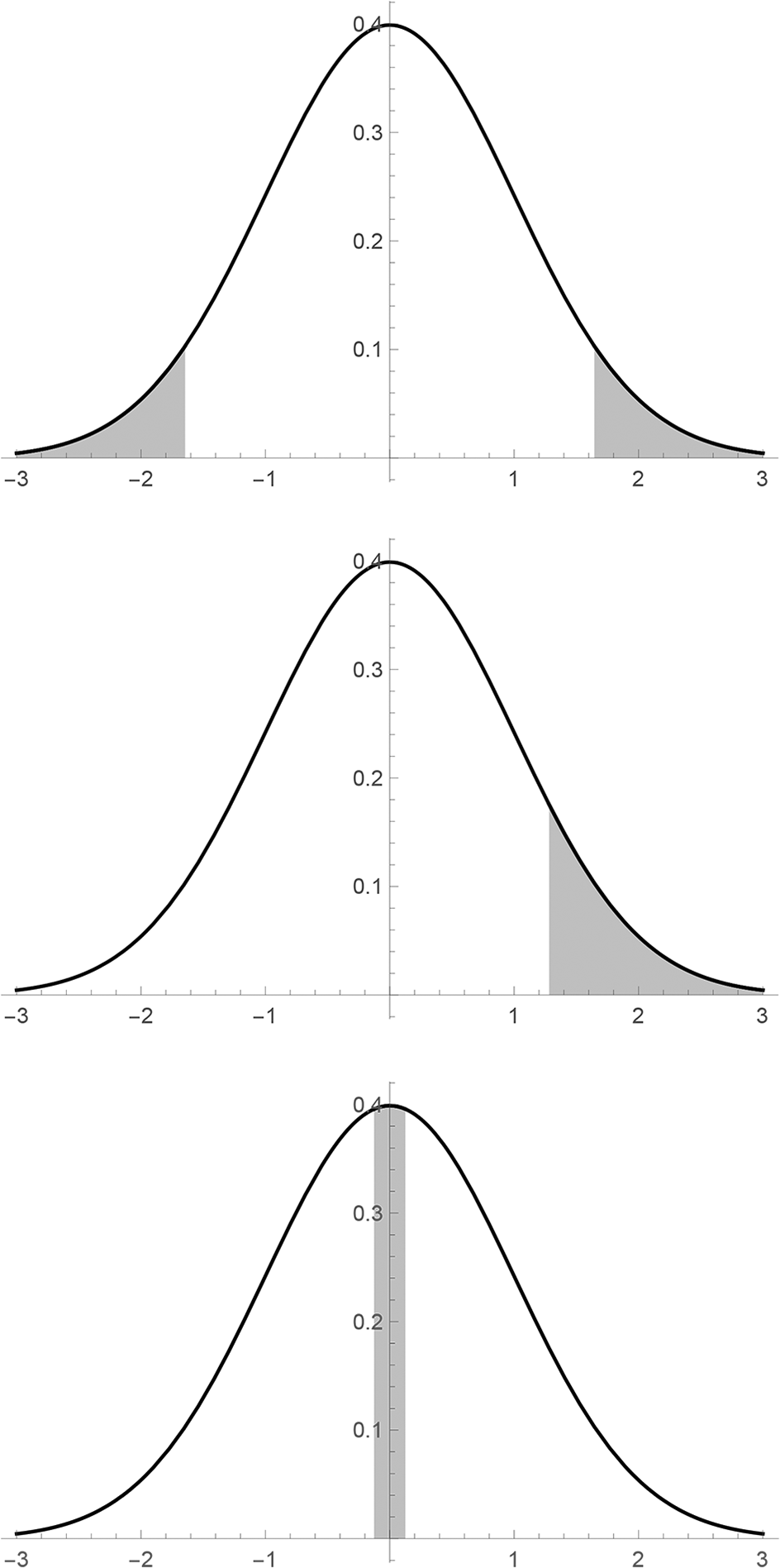
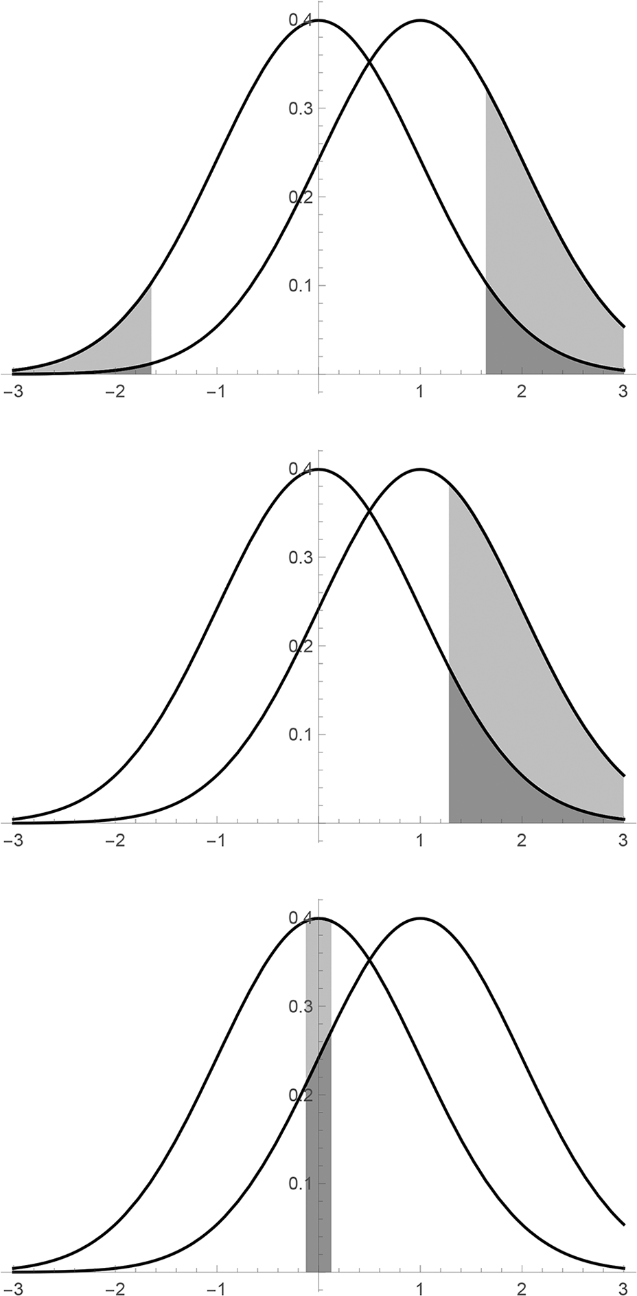
 and the null hypothesis yields a normal distribution with mean 0 and variance 1 over the sample space ℝ, the three regions depicted in figure 4 all meet said requirement.
Three possible rejection regions of size 0.1 for the null hypothesis, R 1, R 2, and R 3.

The solution, according to Neyman and Pearson, is to consider the probability of making a type 2 error. Relative to some alternative hypothesis
 , the probability of rejecting the null hypothesis on the assumption that H is true (and hence H 0 is false) is given by
 . In order to minimize the risk of making a type 2 error, we want this probability to be as high as possible. Consider figure 5. Suppose the alternative hypothesis H 1 yields a normal distribution with mean 1 and variance 1. Then
 . Hence, with H 1 considered as the alternative hypothesis, region R 2 is clearly the better choice. One can even show that, for every alternative region R such that
 and
 , we have
 . In this sense, R 2 dominates every other rejection region. It is a so-called most powerful test of size α for H 0 against the alternative H 1. As a matter of fact, R 2 is a most powerful test of size α against every alternative hypothesis yielding a normal distribution with a mean above 0 and variance 1. Against this particular set of alternative hypotheses, R 2 is a so-called uniformly most powerful test of size α for H 0. Intuitively, R 2 thereby makes for a natural nonarbitrary choice of rejection region. Indeed, it is the one Neyman and Pearson recommend. From a Bayesian point of view, they even show that such a rejection region is optimal independently of prior probabilities in the sense that, whatever the prior probabilities on hypotheses are, the probability of making a type 2 error can only increase by switching to another rejection region of the same size (Neyman and Pearson Reference Neyman and Pearson1933b).
R 2 is a most powerful test of size 0.1 for H 0 against H 1.

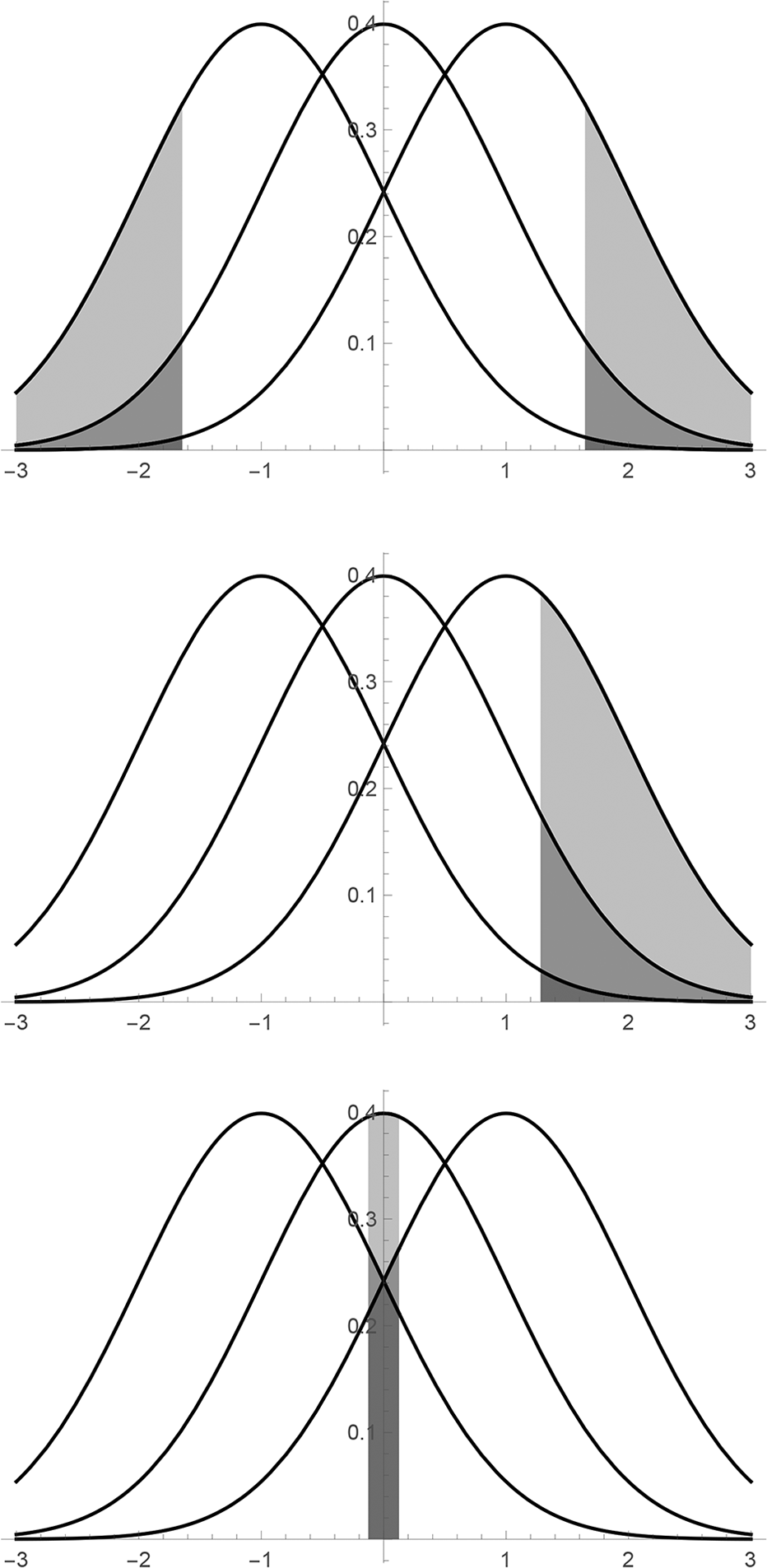
Sometimes, however, no uniformly most powerful test exists. For instance, in the presence of an alternative hypothesis H −1 yielding a normal distribution with mean −1 and variance 1, R 2 is dominated by R 1, as can be seen in figure 6. Hence, against any set of alternative hypotheses including both H 1 and H −1, no uniformly most powerful test exists for H 0. This fact, of which Neyman and Pearson were aware, limits the applicability of their method. The lack of a uniformly most powerful tests in certain situations is a problem for classical statistics, but not one I address in this article.
R 2 is not a most powerful test for H 0 against H −1 (R 1 is more powerful).

3. Bayesian Statistics
Compared with its classical counterparts, Bayesian statistics is straightforward. Basically, it falls out from the more general Bayesian theory of rational degrees of belief (rational credences), composed of the following two postulates:
1. Rational credences are coherent (in the sense of satisfying the laws of probability).
2. Rational credences are updated by conditionalizing on evidence.
However, the theory only tells us how to rationally adjust our prior credences in relation to new evidence. It does not tell us what our prior credences should be. Hence, it does not tell us in absolute terms what our posterior credences should be in relation to new evidence. Unlike classical statistics, it does not tell us whether a particular hypothesis should be rejected.
Initially, this may lead one to suspect that classical statistics harbors some implicit assumptions about what kind of prior credences one may have. On this picture, a classicist would just be a Bayesian with a particular kind of prior credences. As we will see, however, matters are much worse. We we will show that, in a certain rather natural sense, there are situations in which classical and Bayesian statistics are incompatible.
I now present what I take to be the essence of Bayesian statistics. For technical reasons, one usually distinguishes between the case when the set of hypotheses is countable (the discrete case) and when it is continuum sized (the continuous case). For our purposes, it is enough to consider the discrete case. Thus, let Θ be a countable nonempty set of hypotheses, each of which is associated with a probability function
 on an event space Σ (just as in classical statistics), and let
 be a probability function representing the prior credence in each hypothesis. The idea is to extend this function to the mixed domain
 by something like the principal principle (Lewis Reference Lewis and Jeffrey1980). Hence, we assume that, for each event
 and hypothesis
 ,

and, for each
 ,

For the sake of legibility, we write Cr(E&H) instead of Cr(〈E, {H}〉) and Cr(H) instead of Cr({H}). For the same reason, we write Cr(E&Δ) instead of Cr(〈E,Δ〉).
Now, for any observation
 such that
 , the posterior credence CrE is then given for each
 by conditionalizing on E:

The following fact is easy to establish and will be used in the next section:
Fact 1. Provided that
 , we have
 if, for all
 ,
 . Likewise, we have
 if, for all
 ,
 .
4. Agreement
In order to compare classical and Bayesian statistics, let us assume that we have a situation in which there is a uniformly most powerful test for the null hypothesis against the alternatives. We focus on the Neyman-Pearson version of classical statistics but also say something about Fisher’s version as we go along. Now, a classical statistician is not in the business of assigning rational credences to hypotheses. One may still wonder: Are there any credences he might have that would (in some suitable sense of the word) agree with his statistical methods? In the discrete case, the following definition of agreement seems natural.
Definition 1 (Agreement). Let Θ be a countable nonempty set of hypotheses, each of which is associated with a probability function
 on an event space Σ, and let
 be a probability function representing the initial credences of the Bayesian. Assume that the null hypothesis
 has uniformly most powerful test
 of size
 . We then say that the Bayesian and the classicist agree (with respect to α) just in case there is no event
 such that
 but
 .
In plain English: the Bayesian and the classicist agree just in case there is no observation prompting the classicist to reject the null hypothesis while prompting the Bayesian to increase his credence in it.
Observe that, by (4), if
 or
 , then the Bayesian and the classicist will agree trivially, since
 for all
 for which CrE is defined. They will also agree trivially when
 , since that means
 for any
 . What we are interested in is of course whether they can agree nontrivially. By fact 1, it follows that nontrivial agreement is guaranteed in the situation depicted in figure 5, with rejection region R 2 for H 0 against H 1. However, for any given
 , there are situations in which the Bayesian and the classicist cannot agree nontrivially. Here is such an example.
Example 2. Suppose you want to test the null hypothesis (H 0) that
 of all members of a population have property F against the alternative hypothesis (H 1) that
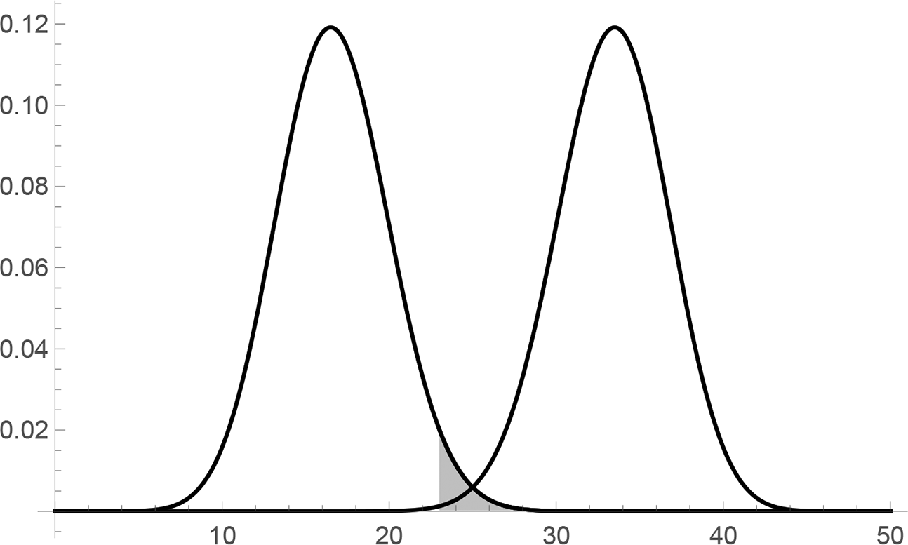
 have it. You decide to perform a random sample of 50 individuals and count the number of F’s in that sample. The expected number of F’s according to each hypothesis is given by a binomial distribution, depicted in figure 7. A most powerful test for the null hypothesis of size 0.05 against the alternative is an event when the sample contains anything between 23 and 50 F’s. Let E be the event that the sample contains 23 F’s. Thus, using a test of size 0.05, the event E should lead to a rejection of the null hypothesis. However, since
 , it follows by fact 1 that nontrivial agreement is impossible. Whatever his prior credences are (assuming that
 ), the Bayesian will deem the null hypothesis more likely after observing E than before.
Expected number of F’s in a random sample of 50 individuals according to the null hypothesis (left) and the alternative hypothesis (right). A most powerful test of size 0.05 for the null hypothesis against the alternative is indicated by the shaded area. In this case, Bayesians and classicists cannot agree.

Clearly, for any
 , a similar situation may arise if we make the sample size n large enough. Likewise, in the case of Fisher’s theory of p-values, assuming that
 just in case
 for any
 , we can for any
 find a large enough sample size n for which an event E exists whose p-value is below α, although the event in question will prompt the Bayesian to increase his credence in H 0. This is essentially just a version of Lindley’s (Reference Lindley1957) paradox. In the original paradox, however, a null hypothesis H 0 is tested against a set of alternatives
 (or, as statisticians like to put it, a precise null hypothesis is tested against an imprecise or composite alternative). In order to generate the original paradox (i.e., in order to derive the conclusion that the Bayesian will increase his credence in the rejected null hypothesis), one has to assume that the Bayesian assigns a nonzero prior credence to it. But since the set of hypotheses is uncountable, this assumption is not very plausible, and it is possible to obtain agreement by simply denying it. In that case, the result is perhaps less problematic for the classicist. According to Spanos (Reference Spanos2013), it merely reveals that powerful tests are more sensitive, which is why we can use them to detect small changes in a population. Moreover, as argued by Sprenger (Reference Sprenger2013), the original paradox may also be a problem for the Bayesian. But in the example at hand, in which a precise null hypothesis is tested against an equally precise alternative, the result is more clearly problematic only for the classicist. Intuitively, there is no sense in which the observation of 23 F’s favors the alternative H 1 over H 0.
The example indicates that, from a classical point of view, it may be unwise to settle for any particular test size in advance (e.g.,
 ), regardless of how small it is. Indeed, for any particular sample size n, there is a most powerful test of some size (e.g.,
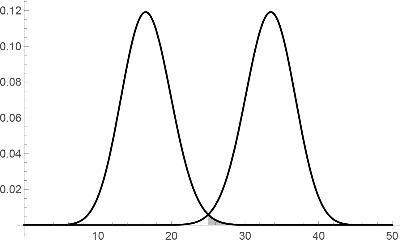
 when
 ) for H 0 against H 1 with respect to which Bayesians and classicists can and, in fact, must agree. Such a situation is depicted in figure 8. According to Mayo and Spanos (Reference Mayo and Spanos2006, 345 n. 21), some statisticians have even suggested that the significance level should be adjusted as a function of the sample size.Footnote 1 As a general solution, however, that suggestion is problematic. As witnessed by the following example, it is possible to construct a situation in which there is no
 with respect to which Bayesians and classicists can agree.
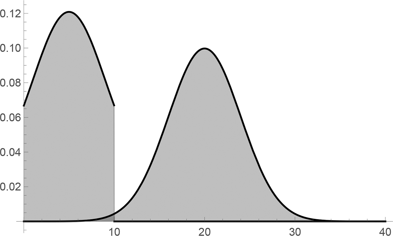
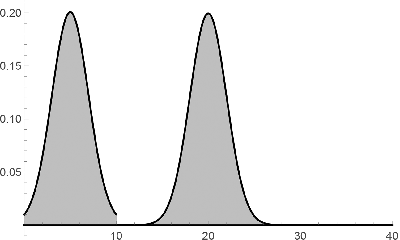
Example 3. Let the null hypothesis H 0 be that the length of individuals in a certain population ranges between 0 and 10 and that it is (approximately) normally distributed with mean 5 and some variance v. Let the alternative hypothesis H 1 be that it ranges between 0 and 40 and that it is (approximately) normally distributed with mean 20 and the same variance v. The situation is depicted in figure 9. According to the null hypothesis, the average length of a random sample will range between 0 and 10 and be (approximately) normally distributed with mean 5 and some variance
 . According to the alternative, it will range between 0 and 40 and be (approximately) normally distributed with mean 20 and the same variance v′. The situation is depicted in figure 10. Clearly, for any
 , a most powerful test of size α of the null hypothesis against the alternative is given by the rejection region [a, 40], for some
 . However, for each such region R, there is an event
 such that
 , namely,
 . Hence, by fact 1, for each
 , nontrivial agreement is impossible.
Most powerful test of size 0.02 for the null hypothesis (left) against the alternative (right) is indicated by the shaded area. In this case, Bayesians and classicist must agree.

Distribution of length in a population according to the null hypothesis (left) and the alternative (right).

Distribution of average length of a random sample according to the null hypothesis (left) and the alternative (right).

The general features making nontrivial agreement impossible in this example are as follows. The null hypothesis is associated with a probability density function f on a sample space
 , where
 , such that
a)
 for all
, and
b) each alternative hypothesis is associated with a probability density function g on the sample space such that
i)
for all
, andii)
is strictly decreasing on [p, q].


Features a and b.ii guarantee that, for each
 , a uniformly most powerful test of that size is given by the interval [a, r], for some
 . Feature b.i guarantees that the event
 is more probable according to the null hypothesis than according to any alternative. By fact 1, this event will therefore prompt the Bayesian to increase his credence in the null.
In summary, the example describes a situation in which, for each
 , there is a most powerful test of size α of the null hypothesis against the alternative and for which there is an event E such that
1. The null hypothesis is rejected by E according to the Neyman-Pearson theory,
2. The p-value of E is smaller than α according to Fisher’s theory,Footnote 2 and
3. Conditionalizing on E will increase one’s credence in the null hypothesis given any nontrivial assignment of prior credences to the null hypothesis and its alternative.
The upshot is that, if we assume that a classical statistician is not allowed to increase his credence in the null hypothesis after he has rejected it, he either has to have trivial or incoherent credences to begin with or fail to update his credences by conditionalization.
Some classicists might respond that although an event with a sufficiently low p-value always indicates some discrepancy from the null, it does not indicate the large discrepancy represented by the alternative in this case. The problem with this response is that, under the assumptions in the case at hand, any discrepancy from the null entails the alternative. So anything indicating the former indicates the latter. Alternatively, they might argue that the testing of a precise null hypothesis against an equally precise alternative is “artificial” or “illegitimate” (e.g., Mayo and Spanos Reference Mayo and Spanos2006, Reference Mayo, Spanos, Bandyopadhyay and Forster2011). If so, I fail to see in what sense. Surely it is possible to know that either of two such hypotheses obtain and to gather evidence for or against them by means of random sampling. A general theory of statistical inference should be able to explain how and why.
5. A Diagnosis
Examples 2 and 3 illustrate (as does Lindley’s paradox) a basic conflict between classical and Bayesian statistics. The conflict is that the former (in the case of Neyman and Pearson, where
 is a uniformly most powerful rejection region) equates the evidential value of a piece of information
 to the evidential value of
 or (in the case of Fisher) equates it to the evidential value of E or something more extreme. Their evidential values are equated in the sense that they license exactly the same classical statistical inferences: respectively, E is sufficient for rejecting the null hypothesis just in case
 is, and the p-value of E is the same as the p-value of E or something more extreme. But E is generally not the same information as
 or E or something more extreme. For the Bayesian, they generally do not have the same evidential value. The point is a familiar one. Jeffreys (Reference Jeffreys and Zellner1980, 453) put it this way: “I have always considered the arguments for the use of [p-values] absurd. They amount to saying that a hypothesis that may or may not be true is rejected because a greater departure from the trial value was improbable [under that hypothesis]; that is, that it has not predicted something that has not happened.”Footnote 3 Indeed, as the examples show, the null hypothesis may assign an arbitrarily low probability to E or something more extreme and yet assign a higher probability to E than any alternative hypothesis. By fact 1, the Bayesian will then increase his credence in the null hypothesis (given any nontrivial prior credences) although it is been rejected by the classicist.
6. Conclusion
Suppose that a classical statistician is not allowed to have a higher degree of belief (credence) in a null hypothesis after he has rejected it than before. We have shown that, in certain situations, he has to either have trivial or incoherent credences to begin with or fail to update his credences by conditionalization. Remember that, in the trivial case, he is either absolutely certain that the null hypothesis is true or absolutely certain that it is false. For obvious reasons, that case is irrelevant in this context. In the nontrivial case, there are plenty of good arguments to the effect that the classical statistician is irrational. I am thinking primarily of synchronic and diachronic Dutch book arguments, which I will not rehearse here. At any rate, there is a conflict between classical statistics and the Bayesian theory of rational degrees of belief.