
1. Introduction
Turbulence, the chaotic state of fluid flow in terms of pressure and velocity, is one of the most challenging fluid physics problems. A fundamental understanding of turbulence physics is essential for designing engineering systems because turbulence exists in nearly all macro engineering and atmospheric flows (Pope Reference Pope2000). Traditionally, researchers have broadly classified the means to study turbulent flows into analytical theory, physical experiment and numerical simulation (Scheffel Reference Scheffel2001).
Navier–Stokes equations are widely used to model turbulent flows such as hurricanes, ocean currents and flows behind high-speed vehicles. However, analytical solutions to Navier–Stokes equations have only been attainable with many assumptions, such as one-dimensional (1-D) geometry, constant specific heats, constant viscosity or equation linearization. However, experiments are often costly and face challenges to collect comprehensive information of the laminar–turbulent transition process and many turbulent quantities, such as the spanwise normal stress, turbulent kinetic energy dissipation and higher-order correlations. Certain unmeasurable flow properties in the flow field can be approximated by strong Reynolds analogy (SRA) (Morkovin Reference Morkovin1962; Cebeci & Smith Reference Cebeci and Smith1974) or extended strong Reynolds analogy (ESRA) models (Bradshaw Reference Bradshaw1977; Gaviglio Reference Gaviglio1987; Barre, Quine & Dussauge Reference Barre, Quine and Dussauge1994; Lele Reference Lele1994; Huang, Coleman & Bradshaw Reference Huang, Coleman and Bradshaw1995; Duan & Martin Reference Duan and Martin2011; Zhang et al. Reference Zhang, Bi, Hussain and She2014; Barre & Bonnet Reference Barre and Bonnet2015), but with strict conditions such as insignificant temperature and density fluctuations. In contrast, the numerical simulation of turbulence has become popular owing to the exponential computing power growth in the last several decades. Numerical simulations have empowered researchers and designers to explore deeper and broader into the details of the system behaviour than what experiment can. Based on the degree of the representation of the accuracy and physics, we can classify the numerical simulation methodologies into direct numerical simulation (DNS), large-eddy simulation (LES) and Reynolds-averaged Navier–Stokes (RANS) simulation.
Each numerical simulation approach possesses its own advantages and disadvantages. So far, DNS is only able to simulate simple flow configurations with low Reynolds numbers owing to the limitation in computational resources. The RANS approach is intrinsically less accurate and unable to provide detailed information about the flow field although it is computationally efficient. It is still widely used in engineering practice because the averaged flow field's reasonable prediction is adequate for design. Since the late l950s, RANS modelling has progressed to second-order closure turbulence models. The performance of the second-order closure models manifests a significant improvement over that of simple turbulence models. Studies of some typical RANS models can be found in the literature (Launder, Reece & Rodi Reference Launder, Reece and Rodi1975; Hanjalic & Launder Reference Hanjalic and Launder1976; Launder Reference Launder1989; Sarkar et al. Reference Sarkar, Erlebacher, Hussaini and Kreiss1989, Reference Sarkar, Erlebacher, Hussaini and Kreiss1991; Speziale, Sarkar & Gatski Reference Speziale, Sarkar and Gatski1991; Ristorcelli, Lumley & Abid Reference Ristorcelli, Lumley and Abid1995; Hwang & Jaw Reference Hwang and Jaw1998; Jaw & Chen Reference Jaw and Chen1998a, ; Girimaji Reference Girimaji2000; Yoder Reference Yoder2003; Carlson Reference Carlson2005; Gross, Blaisdell & Lyrintzis Reference Gross, Blaisdell and Lyrintzis2011; Dudek & Carlson Reference Dudek and Carlson2017). The LES approach situates in between DNS and RANS in computational cost. Large-eddy simulation is more accurate and reliable than RANS simulation for turbulent flows in which large-scale unsteadiness is significant, because LES can resolve large-scale structures without modelling (Pope Reference Pope2000). Additionally, LES can provide more insights into fundamental physics owing to the available instantaneous flow structures. Large-eddy simulation has become a desirable approach to study flows dominated by large-scale coherent structures (Pope Reference Pope2000), such as the plane free shear layer.
Recently, owing to the rapid advances in computational power, improved subgrid-scale (SGS) models have been continuously proposed since the first practical SGS model developed by Smagorinsky (Reference Smagorinsky1963). However, none of them has accomplished the combination of accuracy and efficiency to make LES the preferred turbulence modelling approach for engineers and scientists (Burton & Dahm Reference Burton and Dahm2005). Therefore, the development of accurate and efficient SGS models has been a major task. The SGS stresses appear as essential terms for modelling in LES (Vreman, Geurts & Kuerten Reference Vreman, Geurts and Kuerten1997). Thus, intense efforts have been put into developing sophisticated SGS models, which are able to simulate wall-bounded or non-wall-bounded turbulent flows, e.g. the wall-adapting local eddy-viscosity (WALE) and Sigma models (Nicoud & Ducros Reference Nicoud and Ducros1999; Nicoud et al. Reference Nicoud, Toda, Cabrit, Bose and Lee2011). Many researchers attempted to validate the SGS models using DNS data at relatively low Reynolds numbers (Clark, Ferziger & Reynolds Reference Clark, Ferziger and Reynolds1979; Love Reference Love1980; Piomelli et al. Reference Piomelli, Cabot, Moin and Lee1990; Zang, Dahlburg & Dahlburg Reference Zang, Dahlburg and Dahlburg1992; Vreman, Geurts & Kuerten Reference Vreman, Geurts and Kuerten1995a; Vreman et al. Reference Vreman, Geurts and Kuerten1997; Okong'o & Bellan Reference Okong'o and Bellan2004; Selle et al. Reference Selle, Okong'o, Bellan and Harstad2007; Nicoud et al. Reference Nicoud, Toda, Cabrit, Bose and Lee2011). In such SGS model validations, a priori and a posteriori tests (Piomelli et al. Reference Piomelli, Cabot, Moin and Lee1990) are often used. The a priori test is performed by filtering the DNS data to compute the turbulent SGS stresses and comparing these quantities with stresses provided by SGS models (Vreman et al. Reference Vreman, Geurts and Kuerten1995a). However, the a posteriori test involves real LES simulations, and the results are used to compare with DNS data (Vreman et al. Reference Vreman, Geurts and Kuerten1995a). In the present paper, we adopt the a priori test for the SGS model examination.
The evaluation of turbulence models in a spatially developing turbulent free shear layer with naturally developing inflow condition is not currently available in the literature. The performance of some typical turbulence models in the laminar, transition and turbulent regions of such a flow is still unclear. Additionally, the sensitivity of turbulence models to the change of Mach number is not fully understood. In this context, we perform a comparative study of some typical turbulence models using DNS data generated by a high-order discontinuous spectral element method (DSEM) code (Kopriva & Kolias Reference Kopriva and Kolias1996; Kopriva Reference Kopriva1998; Jacobs, Kopriva & Mashayek Reference Jacobs, Kopriva and Mashayek2005). This DSEM code has been employed for LES and DNS of compressible turbulent flows (Ghiasi et al. Reference Ghiasi, Komperda, Li, Peyvan, Nicholls and Mashayek2019; Li et al. Reference Li, Komperda, Ghiasi, Peyvan and Mashayek2019, Reference Li, Peyvan, Ghiasi, Komperda and Mashayek2021) as well as reacting flows (Komperda et al. Reference Komperda, Ghiasi, Li, Peyvan, Jaberi and Mashayek2020). We do not concentrate on numerical methods but systematically examine and compare the characteristic behaviour of several SRA, RANS and LES models for a three-dimensional (3-D), compressible plane free shear layer. This primary objectives of this work are: (1) to identify and explain the performance of the SRA, RANS and SGS models; (2) to provide a basis for future modelling of a spatially developing, compressible free shear flow in the laminar, transition and turbulent regions. The remainder of this paper is organized as follows. First, we provide a brief overview of the DNS data. Then, the comparisons and discussions of different turbulent models are presented. Finally, we provide a summary of the findings.
2. Direct numerical simulation
In this section, we briefly describe the DNS of the 3-D, compressible turbulent plane free shear layer flow that has been reported in detail in our previous papers (Li et al. Reference Li, Komperda, Ghiasi, Peyvan and Mashayek2019, Reference Li, Peyvan, Ghiasi, Komperda and Mashayek2021).
2.1. Compressible Navier–Stokes equations
The compressible Navier–Stokes equations govern the viscous fluid flow and are solved in conservative form. Variables are non-dimensionalized by the reference length,  $L_{f}^*$, density,
 $\rho _{f}^*$, velocity,
 $U_{f}^*$, and temperature,
 $T_{f}^*$. The superscript
 $*$ denotes dimensional quantities and the subscript
 $f$ indicates reference values. The non-dimensionalized variables are defined as
 \begin{equation} \left.\begin{array}{c} x_j = x_j^*/L_f^*,\quad \rho = \rho^*/\rho_f^*, \\ u_i = u_i^*/U_f^*,\quad t = t^*/(L_f^*/U_f^*), \\ T = T^*/T_f^*,\quad p = p^*/(\rho_f^*{U_f^*}^2), \\ \gamma = c_p^*/c_v^*,\quad Pr=c_p^*\mu^*/\kappa^*, \\ M_f = U_f^*/\sqrt{\gamma R^*T_f^*},\quad Re_f = U_f^*L_f^* \rho_f^* / \mu^*, \\ \end{array}\right\} \end{equation}
where  $x_{j}$ is the
 $j$th Cartesian coordinate. Also,
 $p$,
 $\gamma$ and
 $\mu$ are pressure, specific heats ratio and dynamic viscosity, respectively. Moreover,
 $c_{v}$,
 $c_{p}$,
 $\kappa$ and
 $R$ represent the specific heat at constant volume, specific heat at constant pressure, thermal conductivity and gas constant, respectively. The Prandtl number, reference Mach number and reference Reynolds number are respectively indicated by
 $Pr$,
 $M_f$ and
 $Re_{f}$. These lead to the following non-dimensional Navier–Stokes equations, presented in a conservative form in Cartesian tensor notation,
 $$\begin{gather} \frac{\partial \rho}{\partial t} + \frac{\partial ( \rho u_{j} ) }{\partial x_j} = 0 , \end{gather}$$
 $$\begin{gather}\frac{\partial ( \rho u_{i} )}{\partial t} + \frac{\partial ( \rho u_{i} u_{j} ) }{\partial x_j} ={-}\frac{\partial p}{\partial x_i} + \frac{\partial \sigma_{ij}}{\partial x_j} , \end{gather}$$
 $$\begin{gather}\frac{\partial ( \rho e )}{\partial t} + \frac{\partial [ ( \rho e + p )u_{j}]}{\partial x_j} ={-}\frac{\partial q_{j}}{\partial x_j} + \frac{\partial ( \sigma_{ij}u_{i})}{\partial x_j} . \end{gather}$$
Here, the total energy term, viscous stress tensor and heat flux vector are respectively defined as
 $$\begin{gather} \rho e = \frac{p}{{\gamma - 1}} + \frac{1}{2} \rho u_k u_k , \end{gather}$$
 $$\begin{gather}\sigma_{ij} = \frac{1}{Re_{f}} \left(\frac{\partial u_i}{{\partial {x_j}}} +\frac{\partial u_j}{{\partial {x_i}}}-\frac{2}{3}\frac{\partial u_k}{{\partial x_k}} \delta_{ij}\right) , \end{gather}$$
 $$\begin{gather}q_j ={-}\frac{1}{(\gamma-1)Re_{f}Pr M_{f}^2} \frac{\partial T}{\partial x_j} , \end{gather}$$
where  $\delta _{ij}$ is the Kronecker delta. In this study, the specific heat, thermal conductivity and dynamic viscosity of the fluid are assumed to be constant because the temperature fluctuations in all considered simulations are insignificant (
 $< 6\,\%$) (Li et al. Reference Li, Peyvan, Ghiasi, Komperda and Mashayek2021). The equation of state closes the equations mentioned above, and is given as
 \begin{equation} p = \frac{\rho T}{{\gamma M_{f}^2}} . \end{equation}
The total energy can be also expressed as
 \begin{equation} \rho e = \frac{\rho T}{(\gamma-1)\gamma M_{f}^2} + \frac{1}{2} \rho u_k u_k , \end{equation}
which is convenient when applying Reynolds averaging or Favre averaging to the energy conservation equation.
2.2. Discontinuous spectral element method
This work employs the DSEM as the compressible turbulent flow solver (Jacobs et al. Reference Jacobs, Kopriva and Mashayek2005). The physical geometry is partitioned into 3-D hexahedral elements. The DSEM then uses the isoparametric mapping to map each element onto a unit cube in every direction. After mapping, (2.2)–(2.4) read
 $$\begin{gather} \frac{\partial \hat{\rho}}{\partial t} + \frac{\partial \widehat{( \rho u_{j} ) }}{\partial X_j} = 0 , \end{gather}$$
 $$\begin{gather}\frac{\partial \widehat{( \rho u_{i} )}}{\partial t} + \frac{\partial \widehat{( \rho u_{i} u_{j}+p \delta_{ij} )} }{\partial X_j} = \frac{\partial \widehat{\sigma_{ij}}}{\partial X_j} , \end{gather}$$
 $$\begin{gather}\frac{\partial \widehat{( \rho e )}}{\partial t} + \frac{\partial \widehat{[ ( \rho e + p )u_{j}]}}{\partial X_j} ={-}\frac{\partial \widehat{q_{j}}}{\partial X_j} + \frac{\partial \widehat{( \sigma_{ij}u_{i})}}{\partial X_j} . \end{gather}$$
For (2.10),
 \begin{equation} \hat{\rho}= J \rho ;\quad \widehat{( \rho u_{j} )}= J \frac{\partial X_j}{\partial x_i} ( \rho u_{i} ); \end{equation}
for (2.11),
 \begin{equation} \widehat{( \rho u_{i} )}= J ( \rho u_{i} );\quad \widehat{( \rho u_{i} u_{j}+p \delta_{ij} )}= J \frac{\partial X_j}{\partial x_i} ( \rho u_{j} u_{i}+p \delta_{ji} );\quad \widehat{\sigma_{ij}}= J \frac{\partial X_j}{\partial x_i} \sigma_{ji}; \end{equation}
and for (2.12),
 \begin{align} &\widehat{( \rho e )}= J ( \rho e );\quad \widehat{[ ( \rho e + p )u_{j}]}= J \frac{\partial X_j}{\partial x_i} [ ( \rho e + p )u_{i}];\notag\\ &\widehat{q_{j}}= J \frac{\partial X_j}{\partial x_i} q_{i};\quad \widehat{(\sigma_{ij}u_{i})}= J \frac{\partial X_j}{\partial x_i} (\sigma_{ji}u_{j}). \end{align}
In the above equations,  $J$ is defined as (Jacobs Reference Jacobs2003)
 \begin{align}
J(X_1,X_2,X_3) &= \frac{\partial x_1}{\partial
X_1}\left(\frac{\partial x_2}{\partial X_2}\frac{\partial
x_3}{\partial X_3}-\frac{\partial x_2}{\partial
X_3}\frac{\partial x_3}{\partial X_2} \right) - \frac{\partial x_1}{\partial
X_2}\left(\frac{\partial x_2}{\partial X_1}\frac{\partial
x_3}{\partial X_3}-\frac{\partial x_2}{\partial
X_3}\frac{\partial x_3}{\partial X_1} \right) \nonumber\\ &
\quad + \frac{\partial x_1}{\partial
X_3}\left(\frac{\partial x_2}{\partial X_1}\frac{\partial
x_3}{\partial X_2}-\frac{\partial x_2}{\partial
X_2}\frac{\partial x_3}{\partial X_1} \right),
\end{align}
which is the determinant of the Jacobian matrix of the transformation. The term  $\partial X_i / \partial x_j$ denotes the metrics matrix, where
 $x_j$ and
 $X_i$ are the coordinates of the physical and mapped spaces, respectively. The variables with hat
 $\hat { }$ are in the mapped space, whereas those without a hat are in the physical space.
In each mapped element, high-order Lagrange basis functions estimate the primitive variables and the fluxes on the Gauss quadrature and Lobatto quadrature points, respectively. Gauss quadrature and Lobatto quadrature points are respectively defined as
 \begin{equation} X_{j+1/2} = \frac{1}{2} \left\{ 1-\cos\left[\frac{(2j+1){\rm \pi}}{2N}\right]\right\},\quad j = 0, \ldots, N-1 , \end{equation}
and
 \begin{equation} X_{j} = \frac{1}{2} \left\{ 1-\cos\left[\frac{{\rm \pi} j}{N}\right]\right\},\quad j = 0, \ldots, N , \end{equation}
within the unit cube. Here,  $N - 1$ is the polynomial order of the spectral element. For convenience, we refer to
 $N - 1$ as
 $\varsigma$ hereafter. Finally, the primitive variable,
 $\hat {\rho }$, on the Gauss quadrature points, for example, is estimated as
 \begin{equation} \hat{\rho}(X,Y,Z) = \sum_{i=0}^{\varsigma}\sum_{j=0}^{\varsigma}\sum_{k=0}^{\varsigma} \hat{\rho}_{i+1/2,j+1/2,k+1/2}h_{i+1/2}(X) h_{j+1/2}(Y) h_{k+1/2}(Z) . \end{equation}
Here,  $X$,
 $Y$ and
 $Z$ indicate the mapped space coordinates, while
 $h_{j+1/2}$ denotes the Lagrange interpolating polynomial on the Gauss points. A fourth-order low-storage Runge–Kutta scheme (Carpenter & Kennedy Reference Carpenter and Kennedy1994) is adopted for time integration after the viscous and inviscid fluxes are calculated.
2.3. Simulation parameters
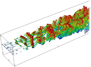
The computational domain, as shown in figure 1, is enclosed with inflow and outflow boundaries (Jacobs, Kopriva & Mashayek Reference Jacobs, Kopriva and Mashayek2003) in the streamwise direction, non-reflecting boundaries (Thompson Reference Thompson1987) in the cross-stream direction and periodic boundaries (Jacobs et al. Reference Jacobs, Kopriva and Mashayek2003) in the spanwise direction. The high- and low-speed streams at the inlet are set to fulfil a velocity ratio,  $VR = 0.54$, which is given as
 \begin{equation} VR = \frac{U_1 - U_2}{U_1 + U_2}= \frac{\Delta U}{U_1 + U_2}.\end{equation}
Three simulations are conducted for various inflow Mach numbers and convective Mach numbers, as given in table 1. The momentum thickness Reynolds number,  $Re_{\theta }$, based on
 $\Delta U$ and
 $\delta _{\theta 0}$, is 140, where
 $\delta _{\theta 0}$ is the initial momentum thickness. The momentum thickness is defined as (Jiménez Reference Jiménez2004)
 \begin{equation} \delta_{\theta} = \frac{1}{\rho_o} \int_{-\infty}^{+\infty} \langle \rho \rangle \frac{\{ u \}-U_2}{\Delta U}\left(1-\frac{\{ u \}-U_2}{\Delta U}\right)\, \mathrm{d} y , \end{equation}
for a spatially evolving compressible plane free shear layer. Here,  $\rho _o$ indicates the initial inflow density, and
 $\langle \rho \rangle$ and
 $\{ u \}$ are respectively the Reynolds-averaged density and Favre-averaged velocity (Favre Reference Favre1969). A pair of angled brackets,
 $\langle \rangle$, denotes a Reynolds average, and a pair of curly brackets,
 $\{ \}$, indicates a Favre average. To compute Reynolds and Favre averages, we start with Reynolds decomposition (Favre Reference Favre1969), which is defined as
 \begin{equation} \phi = \langle \phi \rangle + \phi' , \end{equation}
for any variable  $\phi$. Here,
 $\phi '$ is the turbulent fluctuation from the Reynolds average indicated by the superscript
 $'$. The Reynolds average,
 $\langle \phi \rangle$, can be obtained from an average in time, space or an ensemble average. Similarly, Favre decomposition is defined as (Favre Reference Favre1969)
 \begin{equation} \phi = \{ \phi \} + \phi'' , \end{equation}
where  $\phi ''$ is the turbulent fluctuation with respect to the Favre average denoted by the superscript
 $''$. The Favre average,
 $\{ \phi \}$, is defined as
 \begin{equation} \{ \phi \} = \langle \rho \phi \rangle / \langle \rho \rangle . \end{equation}
Note that
 \begin{equation} \langle \phi'\rangle=0;\quad \langle \rho \phi''\rangle=0;\quad \langle \phi''\rangle\neq 0. \end{equation}
Finally, the specific heats ratio,  $\gamma$, and the reference Prandtl number,
 $Pr_{f}$, are respectively taken as
 $1.4$ and
 $0.7$.
Schematic of the computational domain.

Some simulation parameters and estimated flow properties. Here,  $M_c = \Delta U/(c_1 + c_2)$ (Bogdanoff Reference Bogdanoff1983), where
 $c_1$ and
 $c_2$ are respectively the speeds of sound in the high- and low-speed streams of the shear layer. The inflow Mach numbers on the high- and low-speed sides are respectively indicated by
 $M_1 = U_1/c_1$ and
 $M_2 = U_2/c_2$. Finally,
 $x_R$ represents the location where the transition starts, while
 $x_E$ denotes the location where the transition to turbulent flow ends (see Li et al. (Reference Li, Komperda, Ghiasi, Peyvan and Mashayek2019) for more detail).

2.4. Initial conditions
In this work, the shear layer is formed by two parallel laminar boundary layers, with naturally developing inflow condition and separated by a splitter plate. The two fully developed Blasius boundary layers traverse the trailing edge of the splitter plate and merge into a free shear layer downstream. The configuration of the splitter plate is illustrated in figure 1. A small perturbation is superimposed on the high-speed side boundary layer (Li et al. Reference Li, Komperda, Ghiasi, Peyvan and Mashayek2019). The low-speed stream is laminar without perturbations. The dimensionless density and temperature are uniformly initialized to  $1.0$ and
 $(\Delta U / 2M_c)^2$, respectively. Note that the trace of the initial conditions has been fully purged as the flow attains self-similarity (Bradshaw Reference Bradshaw1966) (see Li et al. (Reference Li, Komperda, Ghiasi, Peyvan and Mashayek2019) for the detailed description of the free shear layer initial conditions).
2.5. Computational domain and grid
All dimensions are normalized by  $\delta _{\theta 0}$. The size of the domain is set as
 $L_x \times L_y \times L_z = 1982 \times 1600 \times 140$, as shown in figure 1. The area of interest is
 $0\leq x \leq 1200$ used for producing DNS data. The remainder is used as a vast buffer zone to avoid solution contamination from cross-stream and outlet boundaries (see figure 1). The computational grid contains 1 368 260 elements and 295 544 160 solution points for a polynomial order of five. With the relatively low Reynolds number (
 $Re = 140$) considered in this work, the resolution of the current grid is sufficient to capture all relevant turbulent scales. A detailed validation against published theoretical, experimental and numerical results has been performed and excellent agreements have been found (Li et al. Reference Li, Komperda, Ghiasi, Peyvan and Mashayek2019). To acquire the necessary statistics, every simulation is first run for five flow-through times to eliminate the transient flow and accomplish a quasi-stationary state. The flow-through time is the time required for the flow to move with the convective velocity from the inlet to the outlet, i.e.
 \begin{equation} \hbox{flow-through time} = \frac{L_x}{U_c} , \end{equation}
where the convective velocity  $U_c$ is defined as
 \begin{equation} U_c = \frac{U_1+U_2}{2},\end{equation}
when the specific heats ratio is assumed to be constant across the shear layer. Second, five flow-through times are required to calculate the first-order statistics. Third, ten flow-through times are needed to acquire sufficient data for the second-order statistics. Finally, we implement post-processing for ensemble averages in the spanwise direction to enhance the accuracy of the statistics. The details of the problem set-up and solution validation are reported in previous work (Li et al. Reference Li, Komperda, Ghiasi, Peyvan and Mashayek2019, Reference Li, Peyvan, Ghiasi, Komperda and Mashayek2021).
3. Strong Reynolds analogy
When developing turbulence models for compressible flows, researchers often start with Morkovin's hypothesis – strong Reynolds analogy (Morkovin Reference Morkovin1962). Morkovin suggested that the effect of high speed is reflected by the change of fluid properties. However, the high-speed effect does not directly affect the dynamic behaviour of turbulence for moderate Mach numbers (Morkovin Reference Morkovin1962). Thus, to properly apply Morkovin's hypothesis, the temperature fluctuations are often required to be negligible, which is valid for the present study. In this section, we examine this hypothesis. In other words, we attempt to show that it is possible to describe turbulent free shear flows using relatively straightforward SRA models.
In the turbulent free shear flow experiment, the measurements might give most of the flow properties in the flow field. However, no direct measurement of temperature fluctuation, or density fluctuation, or the correlation between temperature and velocity or the correlation between density and velocity has been realized. Using the SRA, the temperature and density fluctuations can be obtained from the measured velocity fluctuations. The fluctuations in temperature, density and velocity are related by (Morkovin Reference Morkovin1962; Gaviglio Reference Gaviglio1987; Barre et al. Reference Barre, Quine and Dussauge1994)
 \begin{equation} \frac{\sqrt{\langle T'^{2} \rangle}}{\langle T \rangle} \approx \frac{\sqrt{\langle \rho'^{2} \rangle}}{\langle \rho \rangle}, \end{equation}
and
 \begin{equation} \frac{\sqrt{\langle T'^{2} \rangle}}{\langle T \rangle} = (\gamma-1 )M^2 \frac{\sqrt{\langle u'^2 \rangle}}{\langle u \rangle} , \end{equation}
where  $M = \{u\}/c$ is the local Mach number. Figure 2 shows the variations of the normalized temperature fluctuation,
 $( \sqrt {\langle T'^{2} \rangle }/\langle T \rangle )/(\Delta U)$, and the normalized density fluctuation,
 $(\sqrt {\langle \rho '^{2} \rangle }/\langle \rho \rangle )/(\Delta U)$, across the shear layer. As can be seen, the maximum
 $(\sqrt {\langle T'^{2} \rangle }/\langle T \rangle )/(\Delta U)$ is approximately
 $0.008$ for
 $M_c = 0.3$, and increases to
 $0.011$ as
 $M_c$ increases to 0.7. However, for all cases,
 $\sqrt {\langle T'^{2} \rangle } \ll \langle T \rangle$, which is the condition that satisfies the requirement for applying SRA. Moreover, figure 2 indicates that the variation of the normalized density fluctuation approximately agrees with that of the temperature fluctuation in each case, which confirms the analogy relation defined by (3.1). Moreover, figure 3(a) shows a remarkable agreement between the temperature and velocity fluctuations, which confirms the analogy relation presented by (3.2). However, with increasing convective Mach number,
 $[(\gamma -1 )M^2 \sqrt {\langle u'^2 \rangle } / \langle u \rangle ]/(\Delta U)$ increasingly overpredicts
 $(\sqrt {\langle T'^{2} \rangle } /\langle T \rangle )/(\Delta U)$, as shown in figures 3(b) and 3(c). This trend may arise from the fact that increasing the convective Mach number increases the temperature fluctuation. Consequently, the condition of applying the SRA model deviates away from the ideal assumption.
Cross-stream profiles of the values of the left-hand side (black squares) and right-hand side (red circles) of (3.1) with (a)  $M_c = 0.3$, (b)
 $M_c = 0.5$ and (c)
 $M_c = 0.7$ at
 $x - x_E = 300$. All terms are normalized by
 $(\Delta U)$.

Cross-stream profiles of the values of the left-hand side (black squares) and right-hand side (red circles) of (3.2) with (a)  $M_c = 0.3$, (b)
 $M_c = 0.5$ and (c)
 $M_c = 0.7$ at
 $x - x_E = 300$. All terms are normalized by
 $(\Delta U)$.

Under the condition of negligible temperature fluctuations, the Favre average can be expressed as a function of the Reynolds average and fluctuation (Gaviglio Reference Gaviglio1987; Barre et al. Reference Barre, Quine and Dussauge1994; Barre & Bonnet Reference Barre and Bonnet2015)
 \begin{equation} \{u\} \approx \langle u \rangle + \frac{( \gamma-1 )M^2 }{\langle u \rangle} \langle u'^{2} \rangle, \end{equation}
and
 \begin{equation} \{v\} \approx \langle v \rangle + \frac{( \gamma-1 )M^2 }{\langle u \rangle} \langle u'v' \rangle . \end{equation}
Equations (3.3) and (3.4) represent another form of SRA, which present the relations between the Favre and Reynolds quantities. The compressibility effect is reflected by the square of the Mach number in the equation. Figures 4 and 5 respectively compare the variations of left-hand side (black squares) and right-hand side (red circles) of (3.3) and (3.4). As can be seen, the left-hand side and right-hand side of the equations are in good agreement for various convective Mach numbers. This implies that the SRA performs excellently for different velocity components and convective Mach numbers.
Cross-stream profiles of the values of the left-hand side (black squares) and right-hand side (red circles) of (3.3) with (a)  $M_c = 0.3$, (b)
 $M_c = 0.5$, and (c)
 $M_c = 0.7$, at
 $x - x_E = 300$. All terms are normalized by
 $(\Delta U)$.

Cross-stream profiles of the values of the left-hand side (black squares) and right-hand side (red circles) of (3.4) with (a)  $M_c = 0.3$, (b)
 $M_c = 0.5$, and (c)
 $M_c = 0.7$, at
 $x - x_E = 300$. All terms are normalized by
 $(\Delta U)$.

Although the SRA predicts the relations among the fluctuations of the temperature, density and velocities well, it is insufficient to estimate the budget terms in the turbulent kinetic energy transport equation. Relations must be created for the triple correlations, such as  $\langle \rho u''v'' \rangle$. Those relations are called extended strong Reynolds analogy (ESRA) and can be expressed as (Barre et al. Reference Barre, Quine and Dussauge1994; Barre & Bonnet Reference Barre and Bonnet2015)
 $$\begin{gather} u'' \approx u' - \frac{( \gamma-1 )M^2 }{\langle u \rangle} \langle u'^{2} \rangle , \end{gather}$$
 $$\begin{gather}v'' \approx v' - \frac{( \gamma-1 )M^2 }{\langle u \rangle} \langle u'v' \rangle , \end{gather}$$
 $$\begin{gather}\frac{\langle \rho u''v'' \rangle}{\langle \rho \rangle} \approx \langle \rho u'v' \rangle + \frac{( \gamma-1 )M^2 }{\langle u \rangle} \langle u'^2 v' \rangle - \frac{( \gamma-1 )^2 M^4 }{\langle u \rangle^2} \langle u'^2 \rangle \langle u' v' \rangle . \end{gather}$$
Equations (3.5) and (3.6) express the relations between Favre and Reynolds fluctuations for streamwise and cross-stream velocities. Similarly, (3.7) presents the relation between the density-weighted shear stress term (the shear component in the  $x-y$ plane) and its expression in terms of Reynolds fluctuations. Figure 6 shows the cross-stream profiles of the left-hand side (black squares) and right-hand side (red circles) of (3.7) for
 $M_c = 0.3$,
 $0.5$ and
 $0.7$. The data are extracted at
 $x - x_E = 300$ and normalized by
 $(\Delta U)^2$. It can be seen that the left-hand side and right-hand side are in excellent agreement, which means that the ESRA model correctly estimates the most important component of the production term of the turbulent kinetic energy transport equation.
Cross-stream profiles of the left-hand side (black squares) and right-hand side (red circles) of (3.7) for (a)  $M_c = 0.3$, (b)
 $M_c = 0.5$, and (c)
 $M_c = 0.7$. All terms are extracted at
 $x - x_E = 300$ and normalized by
 $(\Delta U)^2$.

Figures 7 and 8 show the scatter plots of the temporal evolution data of the modelled and DNS Favre velocity fluctuations at a specific location for six flow-through times. Figure 7 compares DNS (left-hand side of (3.5)) with modelled (right-hand side of (3.5)) Favre streamwise velocity fluctuations for  $M_c = 0.3$ and
 $0.7$. All terms are extracted at the centre of the shear layer (see table 2) and normalized by
 $(\Delta U)$. It can be seen that the left-hand side and right-hand side of (3.5) exhibit a high degree of correlation at both
 $M_c = 0.3$ and
 $0.7$. Strong correlation is also found in figure 8 representing (3.6) at the centre of the shear layer. Other locations, such as the upper and lower edges (see table 2) of the shear layer also showed similar behaviours for (3.5) and (3.6). For brevity, the comparisons at these locations are not included here.
Scatter plots of the normalized Favre streamwise velocity fluctuations obtained by DNS (left-hand side of (3.5)) versus that obtained by the models (right-hand side of (3.5)) for (a)  $M_c = 0.3$ and (b)
 $M_c = 0.7$. All terms are extracted at the centre of the shear layer (see table 2) and normalized by
 $(\Delta U)$. The 45-degree line is shown in red.

Scatter plots of the normalized Favre cross-stream velocity fluctuations obtained by DNS (left-hand side of (3.6)) versus that computed by the models (right-hand side of (3.6)) for (a)  $M_c = 0.3$ and (b)
 $M_c = 0.7$. All terms are extracted at the centre of the shear layer (see table 2) and normalized by
 $(\Delta U)$. The 45-degree line is shown in red.


To further compare the discrepancy between the left-hand side and right-hand side of (3.5) and (3.6), we compute the mean absolute deviation (MAD), which is defined as
 \begin{equation} {MAD} = \frac{1}{n} \sum_{i=1}^{n} \lvert LHS_i- RHS_i \rvert , \end{equation}
where  $n$ represents the number of samples. The computed MADs are tabulated in tables 3 and 4. Based on the data in tables 3 and 4, we can conclude the following: the largest correlation discrepancy is located at the centre of the shear layer for both (3.5) and (3.6); the correlation discrepancy in (3.5) is larger than that in (3.6); the error in the high-Mach-number case is higher than that in the low-Mach-number case.


4. Reynolds-averaged Navier–Stokes models
For several decades, the most popular approach for simulating industrial turbulent flows has been the RANS, where the statistical averaging is based on ensemble averaging (Reynolds Reference Reynolds1895). The fundamental approach is to decompose the flow variables into an ensemble mean value component and a fluctuating one, substituting them into the original equations and then ensemble-averaging the resulting equations.
4.1. Reynolds-averaged Navier–Stokes equations
For compressible flows with significant compressibility effects, the averaging is of the Favre type (Smits & Dussauge Reference Smits and Dussauge2006). Note that we let the reference viscosity equal the dimensional viscosity so that the dimensionless viscosity equals one. The non-dimensional Favre-averaged continuity, momentum and energy equations can be respectively written in conservation form as (Huang et al. Reference Huang, Coleman and Bradshaw1995)
 $$\begin{gather} \frac{\partial \langle\rho\rangle}{\partial t}+\frac{\partial \langle\rho\rangle\{u_k\}}{\partial x_k}=0, \end{gather}$$
 $$\begin{gather}\frac{\partial \langle\rho\rangle\{u_i\}}{\partial t}+\frac{\partial \langle\rho\rangle\{u_i\}\{u_k\}}{\partial x_k}={-}\frac{\partial \langle p\rangle}{\partial x_i}+\frac{\partial \langle\tau_{ik}\rangle}{\partial x_k}-\frac{\partial \langle\rho\rangle \{u_i''u_k''\}}{\partial x_k}, \end{gather}$$
 \begin{align} &\frac{\partial }{\partial t}\langle\rho\rangle \left( \frac{\{T\}}{(\gamma-1)\gamma M_{f}^2} + \{K\}+\{k\}\right)+ \frac{\partial }{\partial x_k}\langle\rho\rangle\{u_k\}\left( \frac{\{T\}}{(\gamma-1)\gamma M_{f}^2}+ \frac{\langle p \rangle}{\langle\rho\rangle} + \{K\}+\{k\}\right) \nonumber\\ &\quad = \frac{\partial }{\partial x_k} (\langle\tau_{ik}\rangle\langle u_i\rangle+\langle \tau_{ik}'u_i'\rangle) + \frac{1}{Re_f}\frac{1}{(\gamma-1) M_{f}^2 Pr_{f}}\frac{\partial ^2\langle T\rangle}{\partial x_{k}^2} \nonumber\\ &\qquad -\frac{\partial }{\partial x_k}(\langle\rho\rangle\{u_k''K''\} + \langle\rho\rangle\{u_k''k''\}) - \frac{1}{(\gamma-1) M_{f}^2}\frac{\partial \langle\rho\rangle \{u_k''T''\}}{\partial x_k}, \end{align}
where
 $$\begin{gather} \{k\} = \frac{1}{2} \{u_i''^{2}\} , \end{gather}$$
 $$\begin{gather}\{K\} = \frac{1}{2} \{u_i\}^{2}, \end{gather}$$
 $$\begin{gather}\tau_{ik}' = \frac{1}{Re_f}\left(\frac{\partial u_i'}{\partial x_k}+\frac{\partial u_k'}{\partial x_i} -\frac{2}{3}\frac{\partial u_l'}{\partial x_l}\delta_{ik}\right), \end{gather}$$
 $$\begin{gather}\langle\tau_{ik}\rangle = \frac{1}{Re_f}\left( \frac{\partial \langle u_i\rangle}{\partial x_k} +\frac{\partial \langle u_k\rangle}{\partial x_i} -\frac{2}{3}\frac{\partial \langle u_l\rangle}{\partial x_l}\delta_{ik}\right). \end{gather}$$
In (4.3),  $\{K\}$ and
 $\{k\}$ are the Favre-averaged mean kinetic energy and the Favre-averaged turbulent kinetic energy, respectively. The turbulent transport,
 $\langle \rho \rangle \{u_k''k''\}$, and molecular diffusion,
 $\langle \tau _{ik}'u_i'\rangle$, are typically very small (Speziale et al. Reference Speziale, Sarkar and Gatski1991; Wilcox Reference Wilcox2006), and thus these terms can be neglected. Models for Reynolds stresses,
 $\{u_i''u_k''\}$, and the heat flux,
 $\{u_k''T''\}$, are required to close (4.1)–(4.3) (Wilcox Reference Wilcox2006).
The Reynolds stresses,  $R_{ij}=\{u_i''u_j''\}$, are the components of the second-order tensor, which is intrinsically symmetric, such that
 $R_{ij} = R_{ji}$. The diagonal components are normal stresses, e.g.
 $R_{11}$,
 $R_{22}$ and
 $R_{33}$. The off-diagonal components are shear stresses, such as
 $R_{12}$,
 $R_{13}$ and
 $R_{23}$. The normalized turbulent intensity in different directions can be represented in terms of Reynolds stresses, e.g.
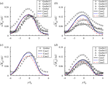
 $\sqrt {R_{ij}}/(\Delta U)$. Figure 9 presents the cross-stream profiles of normalized turbulence intensities from the current DNS and experiments. The compared data are extracted in the self-similar turbulent region. It can be seen that the magnitudes of
 $\sqrt {R_{11}}/(\Delta U)$ and
 $\sqrt {\lvert R_{12}\rvert }/(\Delta U)$ of the current simulations agree well with the experimental results from Goebel & Dutton (Reference Goebel and Dutton1991) for
 $M_c = 0.46$ and 0.69, while
 $\sqrt {R_{33}}/(\Delta U)$ presents good agreement with the experimental result of Gruber, Messersmith & Dutton (Reference Gruber, Messersmith and Dutton1993). The magnitudes of
 $\sqrt {R_{22}}/(\Delta U)$ from the present DNS fall between the experimental results from Goebel & Dutton (Reference Goebel and Dutton1991) for
 $M_c = 0.2$ and 0.46, and are higher than that by Gruber et al. (Reference Gruber, Messersmith and Dutton1993) for
 $M_c = 0.8$. In addition to presenting the cross-stream profiles of turbulence intensities in figure 9, we also tabulate their magnitudes in table 5 for better quantitative comparisons between DNS and experimental results. Particularly note that based on the present DNS results,
 $\sqrt {R_{11}}/(\Delta U) > \sqrt {R_{33}}/(\Delta U) > \sqrt {R_{22}}/(\Delta U)$ for all cases with
 $M_c = 0.3$, 0.5 and 0.7, which indicates that the fluctuations in this work are strongly three-dimensional.
Comparisons of the turbulent intensities, (a)  $\sqrt {R_{11}}/(\Delta U)$, (b)
 $\sqrt {R_{22}}/(\Delta U)$, (c)
 $\sqrt {R_{33}}/(\Delta U)$ and (d)
 $\sqrt {\lvert R_{12}\rvert }/(\Delta U)$ in the self-similar turbulent region between the present and experimental results. Goebel1, Goebel2 and Goebel3 represent the results by Goebel & Dutton (Reference Goebel and Dutton1991) for
 $M_c = 0.2$, 0.46 and 0.69, respectively. Gruber represents the results by Gruber et al. (Reference Gruber, Messersmith and Dutton1993) for
 $M_c = 0.8$. Case1, Case2 and Case3 stand for the present results for
 $M_c = 0.3$, 0.5 and 0.7, respectively.

The turbulence intensities on the centreline of the shear layer for different convective Mach numbers in the self-similar turbulent region.

Reynolds stresses,  $R_{ij}$, are often used to characterize the flow structure motions. The isotropic stress is defined as
 $\frac {2}{3} k \delta _{ij}$; the deviatoric anisotropic part is then defined as (Pope Reference Pope2000)
 \begin{equation} a_{ij} = R_{ij} - \tfrac{2}{3} k \delta_{ij}. \end{equation}
The normalized anisotropy tensor, hereinafter referred to as Reynolds stress anisotropy, is defined as
 \begin{equation} b_{ij} = \frac{a_{ij}}{2k} = \frac{R_{ij}}{R_{ll}} - \frac{1}{3}\delta_{ij}. \end{equation}
Note that in turbulent flows modelling, the Reynolds stress anisotropy tensor  $b_{ij}$ is a significant characteristic of velocity fluctuations (Pantano & Sarkar Reference Pantano and Sarkar2002). In addition, the tensor
 $b_{ij}$ is often used to describe the motions of vortex structures (Smyth & Moum Reference Smyth and Moum2000).
We examine tensor  $b_{ij}$ as a function of the cross-stream coordinate for the self-similar turbulent region. Figure 10 presents comparisons of different components of tensor
 $b_{ij}$ for various convective Mach numbers. At the shear layer centre, the magnitude of
 $b_{11}$ increases significantly, while the magnitudes of
 $b_{22}$ and
 $b_{33}$ slightly increase (more negative) with increasing convective Mach number. This different behaviour is attributed to the fact that the values of Reynolds stresses,
 $R_{22}$ and
 $R_{33}$, decrease as the convective Mach number increases, while the value of
 $R_{11}$ remains almost the same. However, no obvious trend can be found with respect to the effect of compressibility on
 $b_{12}$.
Comparisons of the cross-stream profiles of (a)  $b_{11}$, (b)
 $b_{22}$, (c)
 $b_{33}$ and (d)
 $b_{12}$ in self-similar turbulent region for
 $M_c = 0.3$, 0.5 and 0.7.

Figure 10(a) shows that the positive values of  $b_{11}$ distribute around the centre and edges of the shear layer owing to the dominance of the streamwise component of the velocity fluctuations at these areas. In contrast, two regions in the cross-stream profile show near zero
 $b_{11}$. One region is laterally above the centre of the shear layer, between the high-speed free-stream and the upper shear layer; another region is laterally below the shear layer, between the low-speed free-stream and the lower shear layer. The value of
 $b_{11}$ near zero means the normal Reynolds stress,
 $R_{11}$, is similar in magnitude to the average of
 $R_{22}$ and
 $R_{33}$. It indicates that the regions with near zero
 $b_{11}$ contain the velocity fluctuations which are similar in different directions. Similar discussions hold true for figures 10(b) and 10(c). Figure 10(d) reveals strong negative
 $b_{12}$ at the centre of the shear layer. The strong negative correlation between the streamwise and cross-stream velocity fluctuations indicates that these fluctuations are structured to facilitate the dissipation of energy from the shear layer (Smyth & Moum Reference Smyth and Moum2000).
The Reynolds stress anisotropy tensor,  $b_{ij}$, and the Reynolds stress tensor,
 $R_{ij}$, can be related to each other through
 \begin{equation} R_{ij} = 2k \left( \frac{1}{3}\delta_{ij}+b_{ij}\right). \end{equation}
In the following, we describe several approaches for determining Reynolds stress tensor,  $R_{ij}$. The transport equation of the Reynolds stress tensor can be written as (Pantano & Sarkar Reference Pantano and Sarkar2002)
 \begin{equation} \frac{\partial \langle\rho\rangle R_{ij}}{\partial t}+\frac{\partial \langle\rho\rangle\{u_k\} R_{ij}}{\partial x_k} = \langle\rho\rangle \mathcal{P}_{ij} - \frac{\partial T_{ijk}}{\partial x_k} - \langle\rho\rangle \epsilon_{ij} +\varPi_{ij} + \varSigma_{ij}. \end{equation}
Here, the turbulent production, turbulent transport, turbulent dissipation, pressure–strain correlation and mass flux coupling terms are respectively
 $$\begin{gather} \mathcal{P}_{ij} ={-}\left( R_{ik}\frac{\partial \{u_j\}}{\partial x_k}+R_{jk}\frac{\partial \{u_i\}}{\partial x_k}\right), \end{gather}$$
 $$\begin{gather}T_{ijk}= \langle\rho u_i''u_j''u_k'' \rangle +\langle p'u_i' \rangle \delta_{jk} +\langle p'u_j' \rangle \delta_{ik} - ( \langle \tau_{jk}'u_i'' \rangle + \langle \tau_{ik}'u_j'' \rangle ) , \end{gather}$$
 $$\begin{gather}\epsilon_{ij} = \frac{1}{\langle\rho\rangle} \left\langle \tau_{jk}' \frac{\partial u_i''}{\partial x_k}+\tau_{ik}' \frac{\partial u_j''}{\partial x_k} \right\rangle, \end{gather}$$
 $$\begin{gather}\varPi_{ij} = \left\langle p' \left( \frac{\partial u_i''}{\partial x_j}+\frac{\partial u_j''}{\partial x_i}\right) \right\rangle , \end{gather}$$
 $$\begin{gather}\varSigma_{ij} = \langle u_i'' \rangle \left( \frac{\partial \langle\tau_{jk}\rangle}{\partial x_k}-\frac{\partial \langle p \rangle}{\partial x_j}\right) + \langle u_j'' \rangle \left( \frac{\partial \langle\tau_{ik}\rangle}{\partial x_k}-\frac{\partial \langle p \rangle}{\partial x_i}\right). \end{gather}$$
In the above exact Reynolds stress transport equation, (4.11), the turbulent production term,  $\mathcal {P}_{ij}$, is exact and does not require modelling because the Reynolds stresses and the mean flow velocity are given by the transport equations. Other terms on the right-hand side of (4.11) need modelling. The pressure–strain correlation,
 $\varPi _{ij}$, is the most important term to be modelled (Cecora et al. Reference Cecora, Eisfeld, Probst, Crippa and Radespiel2012).
By setting the indices of (4.11) such that  $j = i$, we can obtain the following transport equation for the turbulent kinetic energy,
 $\{k\} =\frac {1}{2} \{u_i''^{2}\}= \frac {1}{2}R_{ii}$,
 \begin{align}
\frac{\partial \langle\rho\rangle\{k\}}{\partial t}+
\frac{\partial \langle\rho\rangle\{u_k\}\{k\}}{\partial
x_k} &={-}\langle\rho\rangle\{u_i''u_k''\} \frac{\partial
\{u_i\}}{\partial x_k} -\frac{\partial
\langle\rho\rangle\{u_k''k''\}}{\partial x_k}
-\frac{\partial \langle p'u_k'\rangle}{\partial x_k}
+ \frac{\partial \langle\tau_{ik}'
u_i'\rangle}{\partial x_k}\nonumber\\ &\quad -\left\langle\tau_{ik}'\frac{\partial
u_i'}{\partial x_k}\right\rangle -\langle
u_k''\rangle\frac{\partial \langle p\rangle}{\partial x_k}
+\langle u_i''\rangle\frac{\partial
\langle\tau_{ik}\rangle}{\partial x_k} +\left\langle
p'\frac{\partial u_k'}{\partial x_k}\right\rangle.
\end{align}
Based on the literature (Favre Reference Favre1965, Reference Favre1969; Lele Reference Lele1994; Huang et al. Reference Huang, Coleman and Bradshaw1995; Pope Reference Pope2000), the second term on the left-hand side of (4.17) represents kinetic energy convection. The terms on the right-hand side are, respectively, the turbulent production, turbulent convection, pressure transport, viscous diffusion, turbulent viscous dissipation, enthalpic production, compressibility term resulting from turbulent fluctuations and pressure–dilatation correlation. Note that the last three terms are compressibility related terms arising from turbulent fluctuations.
4.2. Formulations of different RANS models
To improve the model accuracy, researchers take higher and higher moments for models, e.g. from the Boussinesq eddy-viscosity approximation, algebraic (zero-equation) models, one-equation models, two-equation models, four-equation models to Reynolds-stress seven-equation models (Pope Reference Pope2000). Consequently, we generate additional unknowns at each level. The purpose of turbulence modelling is to create approximations for the unknowns and finally achieve closure. Most of the compressible turbulence modelling approaches begin with incompressible flows and often provide satisfying results (Smits & Dussauge Reference Smits and Dussauge2006). In contrast to incompressible flows, no model is able to provide accurate results for high compressible flows.
Among various RANS models, the two-equation  $k{-}\epsilon$ model is most commonly used in turbulent free shear flows, while the Reynolds-stress model is currently the most comprehensive turbulent modelling approach (Wilcox Reference Wilcox2006). For the
 $k{-}\epsilon$ model, several unclosed terms in the turbulent kinetic energy transport equation need to be modelled, such as the turbulent kinetic energy dissipation term, turbulent transport terms and compressibility terms resulting from turbulent fluctuations and pressure–dilatation correlation. The turbulent kinetic energy dissipation term is modelled using the hypothesis of high Reynolds numbers, which means the dissipation is assumed to have the form of isotropic dissipation,
 $\epsilon$ (Haase et al. Reference Haase, Aupoix, Bunge and Schwamborn2006). For the modelling of the diffusion terms, the turbulent-transport terms are lumped together and modelled using a classical gradient-diffusion hypothesis (Daly & Harlow Reference Daly and Harlow1970). The model constants associated with the diffusion and dissipation terms are either chosen as constants for the whole flow (Schmidt & Schumann Reference Schmidt and Schumann1989) or calculated dynamically (Ghosal et al. Reference Ghosal, Lund, Moin and Akselvol1995). To account for the compressibility effect, researchers often model the dilatational dissipation term when simulating compressible flows (Sarkar et al. Reference Sarkar, Erlebacher, Hussaini and Kreiss1989, Reference Sarkar, Erlebacher, Hussaini and Kreiss1991; Zeman Reference Zeman1990; Wilcox Reference Wilcox1992). Additionally, the pressure–dilatation correlation, which is the trace of the pressure–strain correlation tensor, plays a key role in the
 $k{-}\epsilon$ model to mimic the influence of compressibility. The functions of the pressure–dilatation correlation in the
 $k{-}\epsilon$ model are similar to that of the pressure–strain correlation in the Reynolds-stress model (Wilcox Reference Wilcox2006).
For the Reynolds-stress model, the unclosed terms in transport equations are turbulent transport terms, dissipation term and pressure–strain correlation. The turbulent transport terms contain contributions of turbulent transport, pressure diffusion and viscous diffusion, where the pressure diffusion term is often considered negligible (Wilcox Reference Wilcox1992). As discussed above, the contributions of turbulent transport terms can be combined and approximated using a generalized gradient diffusion model (Daly & Harlow Reference Daly and Harlow1970). Moreover, the dissipation term is often modelled by an isotropic tensor,  $\epsilon _{ij}=2\epsilon /3$, based on the Kolmogorov hypothesis of local isotropy (Haase et al. Reference Haase, Aupoix, Bunge and Schwamborn2006). An additional transport equation is required to provide the isotropic dissipation term,
 $\epsilon$. Last but not least, the pressure–strain correlation is one of the most important terms in the Reynolds-stress equations for the following reasons. The pressure–strain correlation is mainly responsible for the shear layer growth rate, the turbulence kinetic energy redistribution (Wilcox Reference Wilcox2006) and the influence of compressibility (Pope Reference Pope2000). It also has the same order of magnitude as the production term in the Reynolds-stress equations (see figure 13). In this work, we only consider the assessments of some commonly used dilatational dissipation, pressure–dilatation correlation and pressure–strain correlation models and present them in the following section.
4.2.1. Modelling the dilatational dissipation term
The turbulent dissipation in the turbulent kinetic energy transport equation is also called the scalar dissipation rate,  $\epsilon = \epsilon _{ii}/2 = \langle \tau _{ik}'\partial u_i' / \partial x_k \rangle$. The quantity,
 $\epsilon$, can be decomposed into the solenoidal dissipation,
 $\epsilon _s$, dilatational dissipation,
 $\epsilon _d$, and inhomogeneous dissipation,
 $\epsilon _I$: (Huang et al. Reference Huang, Coleman and Bradshaw1995)
 \begin{equation} \epsilon \approx \epsilon_s+\epsilon_d+\epsilon_I,\end{equation}
where
 $$\begin{gather} \epsilon_s = \frac{2}{Re_f} \langle\omega_{ij}'\omega_{ij}'\rangle, \quad \text{with }\omega_{ij}'=\frac{1}{2} \left(\frac{\partial u_i'}{\partial x_j}-\frac{\partial u_j'}{\partial x_i}\right), \end{gather}$$
 $$\begin{gather}\epsilon_d = \frac{4}{3 Re_f} \left\langle\frac{\partial u_l'}{\partial x_l}\frac{\partial u_k'}{\partial x_k} \right\rangle, \end{gather}$$
 $$\begin{gather}\epsilon_I = \frac{2}{Re_f} \left(\frac{\partial ^2\langle u_i'u_j'\rangle}{\partial x_i\partial x_j} -2\frac{\partial }{\partial x_i}\left\langle u_i'\frac{\partial u_j'}{\partial x_j}\right\rangle\right). \end{gather}$$
The inhomogeneous dissipation mainly arises from the shear between the wall and the shear layer (Brown et al. Reference Brown, Shaver, Lahey and Bolotnov2017; Li et al. Reference Li, Peyvan, Ghiasi, Komperda and Mashayek2021). As expected, the inhomogeneous dissipation is close zero in the turbulence area of the free shear layer (without wall) based on the present DNS data. The inhomogeneous dissipation shows a negligible contribution to the turbulent kinetic energy transport equation in the free shear layer but has a significant contribution in the boundary shear layer (Lele Reference Lele1994; Huang et al. Reference Huang, Coleman and Bradshaw1995; Brown et al. Reference Brown, Shaver, Lahey and Bolotnov2017).
In the  $k{-}\epsilon$ model, the dilatational dissipation term is responsible for the reduction in growth rate as compressibility increases, thus it is a function of turbulent Mach number,
 $M_t = \sqrt {k}/c_{0}$ (Sarkar et al. Reference Sarkar, Erlebacher, Hussaini and Kreiss1989). Here,
 $c_{0} = (c_{1}+c_{2})/2$ is the mean speed of sound. Therefore, the magnitude of the dilatational dissipation term increases with increasing turbulent Mach number. Sarkar et al. (Reference Sarkar, Erlebacher, Hussaini and Kreiss1989) proposed
 \begin{equation} \epsilon_d = M_t^2 \epsilon_s. \end{equation}
The study by Zeman (Reference Zeman1990) suggested
 \begin{equation} \epsilon_d = 0.75\left(1-\exp \left\{ -\left[\frac{M_t-0.1}{0.6} \right]^2 \right\} \right) \epsilon_s. \end{equation}
Later, Wilcox (Reference Wilcox1992) introduced
 \begin{equation} \epsilon_d = 1.5 [M_t^2-0.1^2 ] \epsilon_s. \end{equation}
Figure 11 presents the cross-stream profiles of dilatational dissipation obtained from the present DNS and the models (4.22)–(4.24) for  $M_c = 0.3$ and
 $0.7$. All terms are extracted at
 $x - x_E = 300$ and normalized by
 $(\Delta U)^3/\delta _\theta$. It can be seen that all the models unrealistically overpredict the value of the dilatational dissipation, while the model of Zeman (Reference Zeman1990) (4.23) shows relatively better agreement than the rest for
 $M_c = 0.3$. In the turbulent kinetic energy transport equation, the dilatational dissipation term converts the turbulent kinetic energy to internal energy. The considered models were primarily devised to increase this energy conversion as the convective Mach number increases to account for the compressibility effects. However, in figure 26(c) of our recently published paper (Li et al. Reference Li, Peyvan, Ghiasi, Komperda and Mashayek2021), the ratio of the dilatational to solenoidal dissipation reveals that the value of the dilatational dissipation is insignificant compared with the solenoidal dissipation. In summary, the dilatational dissipation is insignificant in the plane free shear flow for the convective Mach numbers considered in this study. Therefore, the models discussed in this paper for dilatational dissipation are unsuitable for compressible plane free shear layer flows for
 $M_c \leq 0.7$.
Comparison of dilatational dissipation cross-stream profiles between present DNS and models by Sarkar et al. (Reference Sarkar, Erlebacher, Hussaini and Kreiss1989) (4.22), Zeman (Reference Zeman1990) (4.23) and Wilcox (Reference Wilcox1992) (4.24) for (a)  $M_c = 0.3$ and (b)
 $M_c = 0.7$. All terms are extracted at
 $x - x_E = 300$ and normalized by
 $(\Delta U)^3/\delta _\theta$.

4.2.2. Modelling the pressure–dilatation correlation
The pressure–dilatation correlation,  $\varPi = \langle p'({u_k'}/{x_k})\rangle$, is intrinsically the trace of the pressure–strain correlation tensor and appears in the turbulent kinetic energy transport equation. Sarkar, Erlebacher & Hussaini (Reference Sarkar, Erlebacher and Hussaini1992), in their
 $k{-}\epsilon$ two-equation model study, suggested that the pressure–dilatation correlation could be related to the turbulent Mach number, the turbulent kinetic energy production,
 $\mathcal {P}_{kk} = -\langle \rho \rangle \{u_i''u_k''\} ({\{u_i\}}/{x_k})$, and the solenoidal part of the dissipation rate,
 $\epsilon _s = ({2}/{Re_f}) \langle \omega _{ij}'\omega _{ij}'\rangle$, i.e.
 \begin{equation} \varPi ={-}0.15\langle \rho \rangle \mathcal{P}_{kk} M_t+0.2\langle \rho \rangle \epsilon_s M_t^2. \end{equation}
The purpose of including the turbulent Mach number in the model is to account for the effect of compressibility, which may suppress the growth of the shear layer. Later, El Baz & Launder (Reference El Baz and Launder1993) proposed a similar model, which involves the divergence of the Favre average velocity,
 \begin{equation} \varPi = 3\langle \rho \rangle \left( \frac{4}{3} \{k\} \frac{\partial \{u_i\}}{\partial x_i}- \mathcal{P}_{kk} \right) M_t^2. \end{equation}
Huang et al. (Reference Huang, Coleman and Bradshaw1995), based on the study by Sarkar et al. (Reference Sarkar, Erlebacher and Hussaini1992), suggested
 \begin{equation} \varPi ={-}0.4\langle \rho \rangle \mathcal{P}_{kk} M_t^2+0.2\langle \rho \rangle \epsilon_s M_t^2. \end{equation}
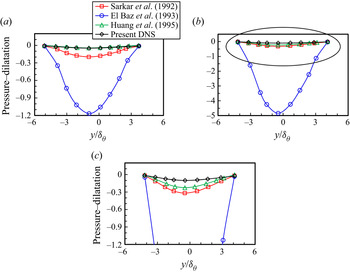
Figure 12 presents the cross-stream profiles from the DNS and the modelled pressure–dilatation correlation. The corresponding data are extracted from the turbulent section of the shear layer at  $x - x_E = 300$. The results of the modelled pressure–dilatation correlation are computed from (4.25) (Sarkar et al. Reference Sarkar, Erlebacher and Hussaini1992), (4.26) (El Baz & Launder Reference El Baz and Launder1993) and (4.27) (Huang et al. Reference Huang, Coleman and Bradshaw1995) for
 $M_c = 0.3$ and
 $0.7$. All these models were mainly designed to decrease the turbulent kinetic energy as the convective Mach number increases to mimic the behaviour of the compressible flow. Based on our previous study (Li et al. Reference Li, Peyvan, Ghiasi, Komperda and Mashayek2021), we conclude that the pressure–dilatation term's contribution to the turbulent kinetic energy budget is insignificant even as the convective Mach number is raised to 0.7, which is consistent with the results by Vreman, Sandham & Luo (Reference Vreman, Sandham and Luo1996). The authors suggested that the pressure–dilatation correlation is negligible in the turbulent kinetic energy transport equation even at the highest Mach numbers examined. This might arise from the self-cancellation when averaging the instantaneous
 $p'({u_k'}/{x_k})$ over time. Therefore, a reliable model should be able to predict that the pressure–dilatation correlation is negligible. Unfortunately, figure 12 shows that the models proposed by Sarkar et al. (Reference Sarkar, Erlebacher and Hussaini1992) and El Baz & Launder (Reference El Baz and Launder1993) largely overestimate the magnitude of pressure–dilatation. Thus, these two models are unsuitable for free shear flows with moderate Mach numbers. However, the model proposed by Huang et al. (Reference Huang, Coleman and Bradshaw1995) shows exceptional performance for
 $M_c = 0.3$ and acceptable prediction for
 $M_c = 0.7$. In conclusion, the model by Huang et al. (Reference Huang, Coleman and Bradshaw1995) provides the best prediction, while the model by El Baz & Launder (Reference El Baz and Launder1993) gives a large overestimate for both
 $M_c = 0.3$ and
 $0.7$. Finally, all considered models show more significant discrepancies with the DNS value as the convective Mach number increases from
 $0.3$ to
 $0.7$.
Pressure–dilatation correlation cross-stream profiles generated by the present DNS and models ((4.25), (4.26) and (4.27)) for (a)  $M_c = 0.3$, (b)
 $M_c = 0.7$ and (c) magnified area from panel (b). All terms are extracted at
 $x - x_E = 300$ and normalized by
 $(\Delta U)^3/\delta _\theta \times 10^{-4}$.

4.2.3. Modelling the pressure–strain correlation
Changes in the pressure–strain correlation components in the Reynolds stress transport equations are responsible for the variations in turbulence structures and free shear layer growth rate (Yoder Reference Yoder2003). The Reynolds stresses decrease with increasing the convective Mach number, but the streamwise normal stress is often less affected (Li et al. Reference Li, Komperda, Ghiasi, Peyvan and Mashayek2019). The pressure–strain correlation components redistribute the turbulence kinetic energy between the streamwise, cross-stream and spanwise components, which increases the anisotropy of the Reynolds stresses (Wilcox Reference Wilcox2006). Hence, to properly account for the variations in Reynolds stresses with increasing convective Mach number, a model capable of predicting the anisotropy of Reynolds stresses is required (Yoder Reference Yoder2003).
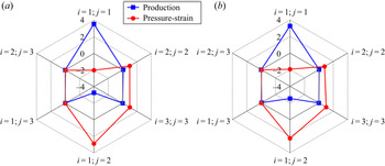
The analysis of the transport equations for the Reynolds stress components may help identify the driving factor behind changes of the Reynolds stresses. Different components of production and pressure–strain correlation for  $M_c = 0.3$ and
 $0.7$ are presented in figure 13. In the streamwise normal stress transport equation (
 $i = 1$ and
 $j = 1$), the production is the dominant source term, while the pressure–strain correlation acts as a sink term. In the cross-stream and spanwise normal stress transport equations (
 $i = 2$ and
 $j = 2$;
 $i = 3$ and
 $j = 3$), however, the production is insignificant and the pressure–strain correlation is the major source term. The shear stress transport equation (
 $i = 1$ and
 $j = 2$) is dominated by the production and pressure–strain correlation terms. In the other shear stress transport equations (
 $i = 1$ and
 $j = 3$;
 $i = 2$ and
 $j = 3$), which involve the shear in the homogeneous direction (spanwise direction), the production and pressure–strain correlation terms appear insignificant. It can be concluded that the pressure–strain correlation term mainly redistributes the turbulence kinetic energy among the normal stresses.
Different components of production and pressure–strain for (a)  $M_c = 0.3$ and (b)
 $M_c = 0.7$. All terms are extracted at
 $x - x_E = 300$ and normalized by
 $(\Delta U)^3/\delta _{\theta }\times 10^{-3}$.

The pressure–strain correlation is one of the essential terms in the Reynolds stress transport equations because it has the same order of magnitude as the turbulent production term (see figure 13). Almost all the pressure–strain correlation models are designed based on the assumption of incompressible and locally homogeneous flows (Yoder Reference Yoder2003). The pressure–strain correlation model devised by Speziale, Sarkar and Gatski (SSG) (Speziale et al. Reference Speziale, Sarkar and Gatski1991) reads
 \begin{align} \varPi_{ij}&
={-}(C_1\langle \rho \rangle \epsilon
+\tfrac{1}{2}C_1^*\langle \rho \rangle \mathcal{P}_{kk}
)\{a_{ij}\}+C_2\langle \rho \rangle\epsilon
(\{a_{ik}\}\{a_{kj}\}-\tfrac{1}{3}\{a_{kl}\}\{a_{kl}\}\delta_{ij})
\nonumber\\ & \quad + (C_3-C_3^*\sqrt{\{a_{kl}\}\{a_{kl}\}}
)\langle \rho \rangle \{k\}\{S_{ij}^*\} \nonumber\\ & \quad
+ C_4\langle \rho \rangle\{k\}(\{a_{ik}\}\{S_{jk}\}
+\{a_{jk}\}\{S_{ik}\}-\tfrac{2}{3}\{a_{kl}\}\{a_{kl}\}\delta_{ij})
\nonumber\\ & \quad + C_5\langle \rho \rangle
\{k\}(\{a_{ik}\}\{W_{jk}\}+\{a_{jk}\}\{W_{ik}\} ).
\end{align}
Here,
 \begin{equation} \{a_{ij}\} = \frac{\{R_{ij}\}}{\{k\}}-\frac{2}{3}\delta_{ij}\end{equation}
is the anisotropy tensor, while
 \begin{equation} \{S_{ij}\} = \frac{1}{2}\left(\frac{\partial \{U_i\}}{\partial x_j}+\frac{\partial \{U_j\}}{\partial x_i} \right)\end{equation}
and
 \begin{equation} \{S_{ij}^*\} =\{S_{ij}\}-\tfrac{1}{3}\{S_{kk}\}\delta_{ij} \end{equation}
are respectively the averaged strain rate and traceless strain rate tensor. Finally,
 \begin{equation} \{W_{ij}\} = \frac{1}{2}\left(\frac{\partial \{U_i\}}{\partial x_j}-\frac{\partial \{U_j\}}{\partial x_i} \right)\end{equation}
is the averaged rotation rate tensor. The isotropic dissipation rate  $\epsilon$ is provided by an additional transport equation. The model coefficients
 $C_1$,
 $C_2$,
 $C_3$,
 $C_4$ and
 $C_5$ are
 $17/10$,
 $21/20$,
 $4/5$,
 $5/8$ and
 $1/5$, respectively. The other two coefficients
 $C_1^*$ and
 $C_3^*$ are set as
 $9/10$ and
 $65/100$, respectively (Speziale et al. Reference Speziale, Sarkar and Gatski1991).
Another pressure–strain correlation model, introduced by Wilcox (Reference Wilcox2006), is also used to close the six Reynolds stress transport equations. For brevity, we refer to Wilcox pressure–strain correlation model as WilcoxRSM hereafter. The WilcoxRSM is given by
 \begin{align} \varPi_{ij} &= \beta^*\widehat{C_1}\omega \left(\langle\tau_{ij}\rangle+\frac{2}{3}\{k\}\delta_{ij}\right)- \hat{\alpha}\left(\mathcal{P}_{ij}-\frac{2}{3}\mathcal{P} \delta_{ij}\right)- \hat{\beta}\left(D_{ij}-\frac{2}{3}\mathcal{P} \delta_{ij}\right) \nonumber\\ & \quad - \hat{\gamma} \{k\} \left(\{S_{ij}\}-\frac{1}{3}\{S_{kk}\}\delta_{ij}\right), \end{align}
with
 \begin{equation} \mathcal{P} = \frac{1}{2}\mathcal{P}_{kk},\quad \omega = \frac{\epsilon}{C_\mu \{k\}},\quad D_{ij} = \langle\tau_{ik}\rangle\frac{\partial \{u_k\}}{\partial x_j}+\langle\tau_{jk}\rangle\frac{\partial \{u_k\}}{\partial x_i}. \end{equation}
The production,  $\mathcal {P}_{ij}$, from (4.12), and the strain rate tensor,
 $\{S_{ij}\}$, from (4.30), are employed in the SSG and WilcoxRSM models. The closure coefficients
 $\beta ^*$,
 $\widehat {C_1}$ and
 $\hat {\alpha }$ are respectively set as
 $9/100$,
 $9/5$ and
 $181/220$, while
 $\hat {\beta }$,
 $\hat {\gamma }$ and
 $C_\mu$ are given as
 $139/220$,
 $59/55$ and
 $9/100$, respectively (Wilcox Reference Wilcox2006).
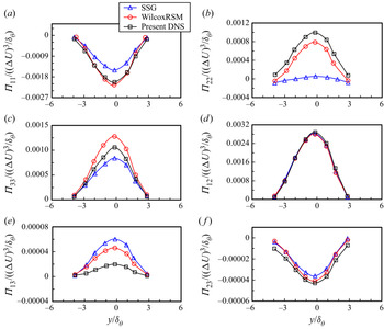
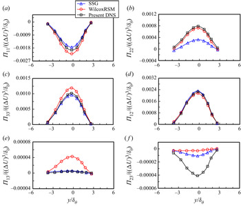
Figure 14 presents the comparison of the cross-stream profiles of DNS and the modelled pressure–strain correlation. All terms are extracted at  $x - x_E = 300$ and normalized by
 $(\Delta U)^3/\delta _\theta$ for
 $M_c = 0.3$. It can be seen from figure 14(a) that the SSG model can roughly predict the sink term, which is the pressure–strain correlation in the streamwise normal stress transport equation (
 $i = 1$ and
 $j = 1$), while the WilcoxRSM model shows excellent estimation. For the cross-stream and spanwise normal stress transport equations (
 $i = 2$ and
 $j = 2$;
 $i = 3$ and
 $j = 3$), the WilcoxRSM model is able to approximately predict the magnitudes of pressure–strain correlation (see figure 14b,c), which acts as the major source term. However, the SSG model underpredicts
 $\varPi _{22}$ (significantly) and
 $\varPi _{33}$ (slightly).
Cross-stream profiles of pressure–strain correlation components (a)  $\varPi _{11}$, (b)
 $\varPi _{22}$, (c)
 $\varPi _{33}$, (d)
 $\varPi _{12}$, (e)
 $\varPi _{13}$ and (f )
 $\varPi _{23}$ computed by models and DNS for
 $M_c = 0.3$. All terms are extracted at
 $x - x_E = 300$ and normalized by
 $(\Delta U)^3/\delta _\theta$.

In contrast, models SSG and WilcoxRSM excellently predict  $\varPi _{12}$ (see figure 14d), which is the dominant term among the six components and has the most significant contribution to the change of Reynolds stresses. The pressure–strain correlation component,
 $\varPi _{12}$, is often used as a primary benchmark to optimize the corresponding models. The last two pressure–strain correlation components,
 $\varPi _{13}$ and
 $\varPi _{23}$, show negligible magnitudes compared with the rest of the components owing to the negligible velocity fluctuation gradient that emerged in the homogeneous spanwise direction. These components are insignificant to the change of the Reynolds stresses. However, both the SSG and WilcoxRSM models can accurately predict the value of
 $\varPi _{23}$ but considerably overpredict
 $\varPi _{13}$.
The performance of the SSG and WilcoxRSM models in the higher convective Mach number case is shown in figure 15, which compares the modelled pressure–strain correlation profiles with the present DNS results for  $M_c = 0.7$. Comparing the performance in the case with
 $M_c = 0.3$, the SSG and WilcoxRSM models show slightly better agreement with the DNS results for components
 $\varPi _{11}$,
 $\varPi _{22}$ and
 $\varPi _{33}$ (see figure 15a–c), while show similar agreements for
 $\varPi _{12}$ (see figure 15d). However, components
 $\varPi _{13}$ and
 $\varPi _{23}$, which are the insignificant ones, are respectively overpredicted and underpredicted by both models. In general, both models can accurately estimate the significant pressure–strain correlation components for
 $M_c = 0.3$ and
 $0.7$, even better for the latter.
Cross-stream profiles of pressure–strain correlation components (a)  $\varPi _{11}$, (b)
 $\varPi _{22}$, (c)
 $\varPi _{33}$, (d)
 $\varPi _{12}$, (e)
 $\varPi _{13}$ and (f )
 $\varPi _{23}$ computed by models and DNS for
 $M_c = 0.7$. All terms are extracted at
 $x - x_E = 300$ and normalized by
 $(\Delta U)^3/\delta _\theta$.

To account for the reduction in the pressure fluctuation with increasing Mach number, a turbulence model for the pressure–strain correlation, including compressibility, is derived by Fujiwara, Matsuo & Arakawa (Reference Fujiwara, Matsuo and Arakawa2000), i.e.
 \begin{equation} (\varPi_{ij})_{comp} = f(M_t)(\varPi_{ij})_{incomp},\end{equation}
where
 \begin{equation} f(M_t ) = 1-\exp \left(-\frac{C_f}{M_t^2} \right).\end{equation}
Here,  $C_f$ is taken as 0.02 for a compressible plane free shear layer (Fujiwara et al. Reference Fujiwara, Matsuo and Arakawa2000). The subscripts
 $comp$ and
 $incomp$ indicate compressible and incompressible, respectively.
In this work, the case with  $M_c = 0.3$ is considered as a reference for the incompressible comparisons owing to the fact that the compressibility effects can be considered negligible for this small convective Mach number (Goebel & Dutton Reference Goebel and Dutton1991; Pantano & Sarkar Reference Pantano and Sarkar2002). Ideally, the pressure–strain correlation in compressible flow (with
 $M_c = 0.7$) can be computed using the compressibility modification model by giving the corresponding
 $M_t$ and the incompressible pressure–strain correlation (with
 $M_c = 0.3$). For brevity, we refer to the compressibility modification model of the pressure–strain correlation (
 $f(M_t)(\varPi _{ij})_{incomp}$) as CMPS.
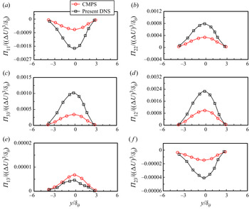
To examine the viability of the CMPS model, we use this model to calculate the pressure–strain correlation for the case with  $M_c = 0.7$, then compare with the primitive DNS results, as shown in figure 16. All terms are extracted at
 $x - x_E = 300$ and normalized by
 $(\Delta U)^3/\delta _\theta$. It can be seen that CMPS unrealistically underestimates all the components of pressure–strain correlation in the case with
 $M_c = 0.7$, except for the component
 $\varPi _{13}$, which is insignificant in the corresponding Reynolds stress transport equation (discussed previously). In summary, the use of the damping function appears to be somewhat unphysical. This compressibility modification model features a dramatic decrease in the magnitude of the pressure–strain correlation. It is suggested that the compressibility effect is caused by suppressing both the pressure–strain correlation and the turbulence anisotropy (Yoder Reference Yoder2003; Cecora et al. Reference Cecora, Eisfeld, Probst, Crippa and Radespiel2012). In that case, the turbulent closure problem becomes much more complicated than the simple damping function approach because the pressure–strain correlation models relate to the second-order terms instead of the scalar terms.
Cross-stream profiles of pressure–strain correlation components (a)  $\varPi _{11}$, (b)
 $\varPi _{22}$, (c)
 $\varPi _{33}$, (d)
 $\varPi _{12}$, (e)
 $\varPi _{13}$ and (f )
 $\varPi _{23}$ computed by CMPS (
 $f(M_t)(\varPi _{ij})_{incomp}$) for
 $M_c = 0.7$. Results from the model are compared with the corresponding DNS (
 $M_c = 0.7$). All terms are extracted from the turbulent region at
 $x - x_E = 300$ and normalized by
 $(\Delta U)^3/\delta _\theta$.

5. Large-eddy simulation models
The DNS data provides the possibility to investigate the robustness of the SGS modelling. This paper only presents the a priori test, using the DNS data of the spatially developing compressible plane free shear layer. Large-eddy simulation is based on the decomposition of a flow variable into resolved and SGS terms (Gullbrand & Chow Reference Gullbrand and Chow2003). To decompose a flow variable, a filtering length scale,  $\varDelta$, is required and is defined as
 \begin{equation} \varDelta = (\varDelta_{x}\varDelta_{y}\varDelta_{z})^{1/3}.\end{equation}
Here,  $\varDelta _{x}$,
 $\varDelta _{y}$ and
 $\varDelta _{z}$ respectively represent the grid sizes in the streamwise, cross-stream and spanwise directions. If the eddy size is larger than
 $\varDelta$, such an eddy is resolved. If the eddy is smaller than
 $\varDelta$, it is modelled (Gullbrand & Chow Reference Gullbrand and Chow2003). In other words, the large-scale structures of the flow is resolved to the grid resolution, while the SGS flow field and its effects on the resolved flow must be modelled. For example, velocity can be decomposed as (Pope Reference Pope2000)
 \begin{equation} u_i = \bar{u}_{i}+u_i'.\end{equation}
Here,  $\bar {u}_{i}$ is the filtered velocity and
 $u_i'$ is the SGS velocity. In the LES models section or hereafter, the superscript
 $'$ indicates the sub-grid scale. Note that the LES decomposition of resolved and SGS velocities should not be confused with the RANS decomposition of mean and fluctuation velocities. The filtered velocity can be written in terms of a convolution integral as (Pope Reference Pope2000)
 \begin{equation} \bar{u}_{i}(x,t) =\int_{\varOmega} u_{i}(\zeta,t)G(x-\zeta) \, \textrm{d} \zeta, \end{equation}
where  $\zeta$ is the dummy variable,
 $G$ indicates the filter kernel for the flow field and
 $\varOmega$ denotes the computational domain. The Favre filtering operation is often applied for compressible turbulence (Favre Reference Favre1983), i.e.
 \begin{equation} \widetilde{u_i} = \frac{\overline{\rho u_i }}{\bar{\rho}}, \end{equation}
where the overbar and tilde denote the Reynolds and Favre filtering operations, respectively. Before writing the LES equations, the LES filtering properties should be defined. Unlike RANS averaging, in LES (Ghosal & Moin Reference Ghosal and Moin1995),
 \begin{equation} \bar{\bar{f}} \neq \bar{f} \quad \textrm{and} \quad \overline{f'} \neq 0 , \end{equation}
where  $f$ is any flow variable. It indicates that averaging a flow field a second time can not reproduce the original averaged flow field.
The filtering method used in this work is nodal filtering (Ghiasi et al. Reference Ghiasi, Komperda, Li, Peyvan, Nicholls and Mashayek2019). To obtain a filtered value of a variable with a polynomial order  $\varsigma$, we first interpolate the variable to a grid with a lower-polynomial order
 $\varsigma '$ such that
 $\varsigma '<\varsigma$. The resulting value is then projected back onto the original grid with the polynomial order of
 $\varsigma$ (Bouffanais et al. Reference Bouffanais, Deville, Fischer, Leriche and Weill2006). The nodal filter is also called an interpolant-projection filter (Ghiasi et al. Reference Ghiasi, Komperda, Li, Peyvan, Nicholls and Mashayek2019). This filter functions as a dampener that reduces high-frequency oscillations caused by the
 $N_f$ highest-frequency modes in the computational domain. Here,
 $N_f = \varsigma - \varsigma '$ is the filter strength, which is conceptually equivalent to the filtering length scale mentioned previously (see the study by Ghiasi et al. (Reference Ghiasi, Komperda, Li, Peyvan, Nicholls and Mashayek2019) for a detailed description of the nodal filtering in the context of the spectral element method). In this paper, we use
 $N_{f} = 2$ as the first filter length scale and
 $N_{f} = 3$ as the second one. Note that the DNS was conducted using a polynomial order
 $\varsigma = 5$.
Filtering the Navier–Stokes equations yields the following filtered conservation equations (Vreman et al. Reference Vreman, Geurts and Kuerten1997):
 $$\begin{gather} \frac{\partial \bar{\rho}}{\partial t} + \frac{\partial ( \bar{\rho} \widetilde{u_{j}})}{\partial x_j} = 0 , \end{gather}$$
 $$\begin{gather}\frac{\partial ( \bar{\rho} \widetilde{u_{i}} )}{\partial t} + \frac{\partial ( \bar{\rho} \widetilde{u_{i}} \widetilde{u_{j}} ) }{\partial x_j} ={-}\frac{\partial \bar{p}}{\partial x_j} - \frac{\partial \tau_{ij}^{sgs}}{\partial x_j}+\frac{\partial \overline{\sigma_{ij}}}{\partial x_j} . \end{gather}$$
In this paper, we only consider modelling the SGS term in the momentum equation. The exact SGS stress tensor,  $\tau _{ij}^{sgs}$ in (5.7), can be expressed as (Vreman et al. Reference Vreman, Geurts and Kuerten1997)
 \begin{equation} \tau_{ij}^{sgs} =\bar{\rho}(\widetilde{u_{i}u_{j}}-\widetilde{u_{i}}\widetilde{u_{j}}). \end{equation}
As can be seen, the correlation term,  $\widetilde {u_{i}u_{j}}$, cannot be obtained from the resolved flow field. The unresolved SGS stress tensor
 $\tau _{ij}^{sgs}$ needs to be modelled to close the equations system. Leonard (Reference Leonard1975) decomposed
 $\tau _{ij}^{sgs}$ into three parts: the Leonard stress,
 $L_{ij}^M$, the cross-SGS stress,
 $C_{ij}^M$, and the Reynolds SGS stress,
 $R_{ij}^M$, i.e.
 \begin{equation} \tau_{ij}^{sgs} = L_{ij}^M+C_{ij}^M+R_{ij}^M , \end{equation}
where
 $$\begin{gather} L_{ij}^M = \bar{\rho}(\widetilde{\widetilde{u_{i}} \widetilde{u_{j}}}-\widetilde{\widetilde{u_{i}}} \widetilde{\widetilde{u_{j}}} ) , \end{gather}$$
 $$\begin{gather}C_{ij}^M = \bar{\rho}(\widetilde{\widetilde{u_{i}}u'_{j}} +\widetilde{u'_{i}\widetilde{u_{j}}} -\widetilde{\widetilde{u_{i}}}\widetilde{u'_{j}} -\widetilde{u'_{i}}\widetilde{\widetilde{u_{j}}}) , \end{gather}$$
 $$\begin{gather}R_{ij}^M = \bar{\rho}(\widetilde{u'_{i}u'_{j}} -\widetilde{u'_{j}u'_{i}}) . \end{gather}$$
From the resolved velocity field,  $\tilde {u}$, Leonard stress components,
 $L_{ij}^M$, can be directly calculated. Leonard stress is often called the outscatter term because the formulation of Leonard stress represents the interaction of two resolved scale structures and such interaction generates small-scale structures. The cross-SGS stress components,
 $C_{ij}^M$, represent the interaction and turbulence energy exchange between large-scale structures and small-scale ones, respectively. However, the net energy exchange is from the large-scale structures to small-scale ones. The Reynolds SGS stress components,
 $R_{ij}^M$, represent the interaction between two SGS stresses and such interaction yields a large-scale structure. This behaviour is also called the backscatter. In contrast to
 $C_{ij}^M$, the
 $R_{ij}^M$ only converts turbulent energy from the small-scale structures to the large-scale ones (Xu Reference Xu2003). Traditionally, researchers separately modelled the Leonard stress, cross-SGS stress and Reynolds SGS stress. However, Speziale (Reference Speziale1985) suggested that modelling the three stresses together can also satisfy the Galilean invariance property.
Piomelli et al. (Reference Piomelli, Cabot, Moin and Lee1991) proposed that the energy transfer between resolved and SGS structures can be represented by the SGS dissipation, i.e.
 \begin{equation} (\epsilon_{SGS})_{ij} = \tau_{ij}^{sgs}\tilde{S}_{ij} , \end{equation}
where
 \begin{equation} \tilde{S}_{ij}= \frac{1}{2}\left(\frac{\partial \widetilde{u_i}}{\partial x_j}+\frac{\partial \widetilde{u_j}}{\partial x_i} \right) . \end{equation}
If  $\epsilon _{SGS}$ is negative, the SGS structures remove energy from the resolved scale structures (forward scatter); if
 $\epsilon _{SGS}$ is positive, SGS structures transfer energy to the resolved scale structures (backscatter). The forward and backward scatters of
 $(\epsilon _{SGS})_{ij}$ respectively indicated by
 $(\epsilon _{ij})_-$ and
 $(\epsilon _{ij})_+$, are defined as (Piomelli et al. Reference Piomelli, Cabot, Moin and Lee1991)
 \begin{equation} (\epsilon_{ij})_-{=} \tfrac{1}{2}((\epsilon_{SGS})_{ij}-\lvert (\epsilon_{SGS})_{ij} \rvert) , \end{equation}
and
 \begin{equation} (\epsilon_{ij})_+{=} \tfrac{1}{2}((\epsilon_{SGS})_{ij}+\lvert (\epsilon_{SGS})_{ij} \rvert) . \end{equation}
Figure 17 illustrates the normalized  $(\epsilon _{SGS})_{11}$,
 $(\epsilon _{SGS})_{22}$,
 $(\epsilon _{SGS})_{33}$,
 $(\epsilon _{SGS})_{12}$,
 $(\epsilon _{SGS})_{13}$ and
 $(\epsilon _{SGS})_{23}$, which are computed from the current DNS data for
 $M_c = 0.3$. The contours in red indicate backscatter, while areas in blue indicate forward scatter (absolute dissipation). It can be seen that all components of SGS dissipation contribute both backward and forward scatter in the vortex structure regions. It indicates that energy actively exchanges between small- and large-scale vortex structures in the shear layer.
Contours of instantaneous SGS dissipation components,  $(\epsilon _{SGS})_{11}$,
 $(\epsilon _{SGS})_{22}$,
 $(\epsilon _{SGS})_{33}$,
 $(\epsilon _{SGS})_{12}$,
 $(\epsilon _{SGS})_{13}$ and
 $(\epsilon _{SGS})_{23}$ computed from DNS data for
 $M_c = 0.3$. All components are extracted in the turbulent region and normalized by
 $(\Delta U)^3$.

5.1. SGS modelling
Most of the LES formulations require SGS stress modelling, and such models are often referred to as SGS models. The SGS models are theoretically simpler and more general than the RANS models because nearly all SGS models are devised for small-scale structures, and the small-scale structures are more isotropic and thus more universal for various flows (Xu Reference Xu2003). We consider four SGS models in this study: the Smagorinsky model (SM), the dynamic Smagorinsky model (DS), the scale similarity model (SS) and the gradient model (GM). The first two models are eddy viscosity type models. The last two models, SS and GM, function as their names suggest, relevant to structure similarity and velocity gradient concepts.
5.1.1. Smagorinsky model
The first practical SGS model is the Smagorinsky model (SM) (Smagorinsky Reference Smagorinsky1963), based on the methodology of the eddy viscosity model:
 \begin{equation} \tau_{ij}^{sgs} - \tfrac{1}{3}\tau_{kk}^{sgs} \delta_{ij} ={-}2\nu_t(\tilde{S}_{ij} - \tfrac{1}{3}\tilde{S}_{kk}\delta_{ij}), \end{equation}
where  $\tau _{kk}^{sgs}$ is the isotropic part of
 $\tau _{ij}^{sgs}$ and
 $\nu _t$ is the eddy viscosity. The eddy viscosity is defined as (Smagorinsky Reference Smagorinsky1963)
 \begin{equation} \nu_t = ( C_t\varDelta)^2 \bar{\rho} \lvert \tilde{S} \rvert , \end{equation}
where the magnitude of the strain rate tensor is
 \begin{equation} \lvert \tilde{S} \rvert = (2 \tilde{S}_{mn}\tilde{S}_{mn})^{1/2} . \end{equation}
Here,  $C_t$ is the Smagorinsky coefficient and is set as a constant.
The Smagorinsky model assumes a proportional relation between the SGS stress tensor and the strain rate tensor. This model, applying the gradient diffusion methodology, is similar to the Boussinesq approximation for RANS models. The coefficient,  $C_t$, can be estimated by analysing the isotropic turbulence decay (Smagorinsky Reference Smagorinsky1963). However, there are many unavoidable limitations when using the Smagorinsky model. The value of
 $C_t$ must be varied for different types of flows (Moin et al. Reference Moin, Squires, Cabot and Lee1991). For example, Lilly (Reference Lilly1966) proposed
 $C_t = 0.23$ in the homogeneous isotropic turbulence, while Deardroff (Reference Deardroff1970) suggested
 $C_t = 0.1$ for a turbulent channel flow. This paper evaluates the Smagorinsky model using the latter value of 0.1 suggested by Deardroff (Reference Deardroff1970). Moreover, the viscous dissipation would not vanish in the laminar region (Moin et al. Reference Moin, Squires, Cabot and Lee1991). Instead, the model would overly dissipate energy in the laminar region and the transition region (Piomelli & Zang Reference Piomelli and Zang1991). Finally, a well-known limitation of this model is that it cannot account for energy backscatter (Moin et al. Reference Moin, Squires, Cabot and Lee1991), which is the process where the turbulent energy transfers from small-scale structures back to large-scale ones.
5.1.2. Dynamic eddy viscosity model
The dynamic eddy viscosity model (DM) (Germano et al. Reference Germano, Piomelli, Moin and Cabot1991) functions as an eddy viscosity model but with a dynamic Smagorinsky coefficient. The dynamic coefficient is obtained based on the scale similarity concepts. This model computes the coefficient both spatially and temporally by using the information in the resolved flow field through two different filter lengths (Xu Reference Xu2003). Therefore, the coefficient is a function of both space and time. Theoretically, the issue of over dissipation in the laminar and transition regions can be addressed by using this model. The dynamic eddy viscosity model by Moin et al. (Reference Moin, Squires, Cabot and Lee1991) is considered in this paper. This model inherits the Smagorinsky model, while a dynamic coefficient of  $C_d$ replaces the square of the constant coefficient
 $C_t$:
 \begin{equation} \tau_{ij}^{sgs} - \tfrac{1}{3}\tau_{kk}^{sgs}\delta_{ij} ={-}2C_d \varDelta^2 \bar{\rho} \lvert \tilde{S} \rvert(\tilde{S}_{ij} - \tfrac{1}{3}\tilde{S}_{kk}\delta_{ij}) . \end{equation}
The Favre filtered SGS stress expression (exact solution) is
 \begin{equation} \tau_{ij}^{sgs} = \bar{\rho}(\widetilde{u_{i}u_{j}}-\widetilde{u_{i}}\widetilde{u_{j}}) = \overline{\rho u_{i}u_{j}}-\frac{\overline{\rho u_i} \overline{\rho u_j}}{\bar{\rho}} . \end{equation}
A test filter is introduced in the dynamic model to bring the information from the resolved field (Germano et al. Reference Germano, Piomelli, Moin and Cabot1991). The test filter width,  $\hat {\varDelta }$, with a larger filter length than the resolved grid filter, is defined similarly as the grid filter width. Applying the test filter to
 $\tau _{ij}^{sgs}$, the mentioned Favre filtered SGS stress expression (5.21) becomes
 \begin{equation} \hat{\tau}_{ij}^{sgs} = \widehat{\overline{\rho u_{i}u_{j}}}-\widehat{\frac{\overline{\rho u_i} \overline{\rho u_j}}{\bar{\rho}}} . \end{equation}
The test filtered stress  $T_{ij}$ is defined similarly as the Favre filtered SGS stress expression (5.21)
 \begin{equation} T_{ij} = \widehat{\overline{\rho u_{i}u_{j}}}-\frac{\widehat{\overline{\rho u_i}}\, \widehat{\overline{\rho u_j}}}{\hat{\bar{\rho}}} \end{equation}
and is modelled as
 \begin{equation} T_{ij} - \tfrac{1}{3}T_{kk}\delta_{ij} ={-}2C_d \hat{\varDelta}^2 \hat{\bar{\rho}} \lvert \hat{\tilde{S}} \rvert(\hat{\tilde{S}}_{ij} - \tfrac{1}{3}\hat{\tilde{S}}_{kk}\delta_{ij}) . \end{equation}
According to Germano's identity (Germano et al. Reference Germano, Piomelli, Moin and Cabot1991), the relation among  $\tau _{ij}^{sgs}$,
 $T_{ij}$ and
 $L_{ij}$ gives
 \begin{equation} L_{ij} = T_{ij}-\widehat{{\tau}}_{ij}^{sgs}= \widehat{\frac{\overline{\rho u_i} \overline{\rho u_j}}{\bar{\rho}}}-\frac{\widehat{\overline{\rho u_i}} \widehat{\overline{\rho u_j}}}{\widehat{\bar{\rho}}}=\widehat{\bar{\rho} \widetilde{u_{i}} \widetilde{u_{j}}}-\frac{\widehat{\overline{\rho u_i}}\, \widehat{\overline{\rho u_j}}}{\hat{\bar{\rho}}}.\end{equation}
Substituting equations (5.20) and (5.24) into (5.25) yields
 \begin{equation} L_{ij} = C_d [{-}2 \hat{\varDelta}^2 \hat{\bar{\rho}} \lvert \hat{\tilde{S}} \rvert(\hat{\tilde{S}}_{ij} - \tfrac{1}{3}\hat{\tilde{S}}_{kk}\delta_{ij}) + \widehat{2 \varDelta^2 \bar{\rho} \lvert \tilde{S} \rvert(\tilde{S}_{ij} - \tfrac{1}{3}\tilde{S}_{kk}\delta_{ij})} ]= C_d M_{ij},\end{equation}
by neglecting the isotropic part of SGS stress tensors –  $\tau _{kk}^{sgs}$ and
 $T_{kk}$. This is because
 $\tau _{kk}^{sgs}$ and
 $T_{kk}$ are not only negligible in terms of their magnitudes but also destabilize the simulation (Moin et al. Reference Moin, Squires, Cabot and Lee1991; Vreman, Geurts & Kuerten Reference Vreman, Geurts and Kuerten1995b).
Applying the least-squares proposed by Lilly (Reference Lilly1992) and spatial averaging, the dynamic coefficient  $C_d$ is defined as
 \begin{equation} C_d = \frac{\langle L_{ij} M_{ij} \rangle }{\langle L_{kl} M_{kl} \rangle} , \end{equation}
where  $\langle \ \rangle$ indicates the spatial averaging over the homogeneous direction (spanwise direction in this paper) of the flow.
5.1.3. Scale similarity model
In LES, backscatter, which does not exist in eddy viscosity models but is an essential feature of SGS stresses, transfers turbulent energy from small-scale structures back to large-scale ones (Bardina, Ferziger & Reynolds Reference Bardina, Ferziger and Reynolds1980). To reproduce such backscatter, Bardina et al. (Reference Bardina, Ferziger and Reynolds1980) introduced the first scale similarity model (SS). This model assumes that the structures of different levels of SGS stresses are similar to the smallest resolved stresses. In other words, the SGS stresses can be predicted based on the resolved flow field. This work examines a modified version of the scale similarity model (Speziale Reference Speziale1985)
 \begin{equation} \tau_{ij}^{sgs} \approx C_L \bar{\rho}(\widetilde{\widetilde{u_{i}}\widetilde{u_{j}}} -\widetilde{\widetilde{u_{i}}}\widetilde{\widetilde{u_{j}}}) = C_L L_{ij}^M, \end{equation}
where  $C_L$ is a similarity coefficient and chosen as unity (Speziale Reference Speziale1985). Here,
 $L_{ij}^M$ is the modified Leonard stress defined in (5.10). Based on the definition, the implementation of the scale similarity model requires second filtering (test filtering) on the resolved flow field.
5.1.4. Gradient model
The Gradient model (GM) relates the SGS stress tensor to the inner product of velocity gradients (Clark et al. Reference Clark, Ferziger and Reynolds1979; Vreman et al. Reference Vreman, Geurts and Kuerten1997)
 \begin{equation} \tau_{ij}^{sgs} \approx \frac{\varDelta^2}{12}G_{ij} , \end{equation}
where
 \begin{equation} G_{ij} = \frac{\partial \widetilde{u_i}}{\partial x_k} \frac{\partial \widetilde{u_j}}{\partial x_k} . \end{equation}
The gradient model is efficient in terms of computational cost owing to its zero-equation nature. Additionally, the velocity derivatives can be reused in the viscous stresses computations (Vreman et al. Reference Vreman, Geurts and Kuerten1997). However, using this model to close the LES momentum equation may result in a negative viscosity (Leonard Reference Leonard1997) and may cause instabilities.
5.2. Comparison with filtered DNS data
The performance of the considered SGS models is studied via the analyses of the correlation coefficient and discrete  $L_2$-norm. The correlation coefficient,
 $R(a,b)$, and discrete
 $L_2$-norm,
 $\Vert a-b\Vert _2$, between two variables (
 $a$ and
 $b$) are respectively defined as (Wright Reference Wright1921; Liu, Meneveau & Katz Reference Liu, Meneveau and Katz1994; Okong'o & Bellan Reference Okong'o and Bellan2004)
 \begin{equation} R(a,b) = \frac{\displaystyle n\sum_{i=1}^{n} a_i b_i - \sum_{i=1}^{n} a_i \sum_{i=1}^{n} b_i}{\displaystyle \sqrt{\left[n\sum_{i=1}^{n} a_i^2 - \left(\sum_{i=1}^{n} a_i \right)^2 \right] \left[n\sum_{i=1}^{n} b_i^2 - \left(\sum_{i=1}^{n} b_i \right)^2 \right] }} , \end{equation}
and
 \begin{equation} \Vert a-b \Vert_2 = \sqrt{\sum_{i=1}^{n}(a_i-b_i)^2}, \end{equation}
where  $a$ and
 $b$ are two arbitrary variables, while
 $n$ is the number of paired samples. Hereafter,
 $R$ represents the correlation coefficient defined by (5.31). The correlation coefficient between the modelled and exact stresses reveals the quality of the modelled spatial structure of the turbulence. The magnitude of
 $R$ ranges from
 $0$ to
 $1$. Magnitudes near unity represent a high correlation (Lu, Rutland & Smith Reference Lu, Rutland and Smith2007). Moreover, the
 $L_2$-norm of the difference between the modelled and exact stresses indicates whether the model accurately predicts the average value of the stress. To better present the
 $L_2$-norm of the difference between the modelled and exact stresses, we normalize it with the
 $L_2$-norm of the exact stress. A normalized
 $L_2$-norm with a significantly less than unity magnitude represents a low relative error.
Owing to the large difference in the behaviours of laminar and turbulent flows, we separately investigate the performance of the SGS models in the laminar, transition and turbulent regions. Based on our previous work (Li et al. Reference Li, Komperda, Ghiasi, Peyvan and Mashayek2019) for  $M_c = 0.3$ and 0.7, the transition approximately starts at 30 and 230, while the turbulence roughly initiates at 340 and 670, respectively (see table 1).
5.2.1. Correlation coefficient
The correlation coefficients,  $R_{ij}$, between the modelled SGS stress components and the corresponding DNS results are presented in figure 18 for the case with
 $M_c = 0.3$. The considered models include SM, DS, SS and GM. It can be seen that the models can provide high correlations for most of the SGS stress components in the laminar region, except model SM for
 $\tau _{12}^{sgs}$ and
 $\tau _{13}^{sgs}$, DS for
 $\tau _{13}^{sgs}$ and SS for
 $\tau _{23}^{sgs}$, which give low correlations. However, model GM, in general, shows high correlations for all of the SGS stress components. This arises from the fact that the inner product of velocity gradients in the laminar region is near-zero. It is well known that the SGS model may overly dissipate energy in the laminar region (Piomelli & Zang Reference Piomelli and Zang1991). The operation of any SGS model should be ideally suspended in the laminar region owing to the absence of small-scale structures.
Correlation coefficient,  $R$, between the exact and the modelled
 $\tau _{ij}^{sgs}$ at the (a) laminar region, (b) transition region and (c) turbulent region for
 $M_c = 0.3$.

For the transition region, we can observe an apparent trend that the correlation increases from model SM, DS, SS to GM, except for  $\tau _{11}^{sgs}$ and
 $\tau _{12}^{sgs}$, where there is a small decrease from model SS to GM. For the three normal stresses, the correlations of models SS and GM are higher than 0.9, which implies that models SS and GM can accurately predict the structures of the SGS stress tensor. This is because both models are designed based on the concept that the SGS stresses are approximated from the resolved flow field.
For the most important region in the computational domain, the turbulent region, models SS and GM give high correlations for most SGS stress components. The trend of increasing correlation from model SM, DS, SS to GM, found in the transition region, is also observed in the turbulent region. In general, the model GM shows the highest correlation compared with the rest, while model SM gives the worst performance. The reasons might be the following: first, isotropic turbulence is the necessary assumption for applying model SM; second, the Smagorinsky coefficient is constant over the entire domain; third, energy only transfers from resolved to SGS structures. We also present correlation coefficients for higher convective Mach number,  $M_c = 0.7$, as seen in figure 19. In the laminar region, unlike the performance shown in the case with
 $M_c = 0.3$, all the models in general provide lower correlations. This trend can be explained with the characteristics of the flow field downstream of the trailing edge of the splitter plate. With the naturally developing boundary inlet condition, boundary layers evolve on the splitter plate, eventually encounter at the trailing edge and form a velocity deficit. The velocity deficit magnitude (VDM) and the velocity deficit presence distance (VDPD) increase as compressibility increases (Li et al. Reference Li, Peyvan, Ghiasi, Komperda and Mashayek2021). These phenomena affect the ability of the considered models to replicate the SGS stress components in the laminar region with high convective Mach numbers because the models are formulated based on the filtered velocity. In contrast, in the transition and turbulent regions, similar trends observed in figure 18 can also be found here. This observation implies that compressibility has an insignificant influence on the correlation coefficients of the SGS models in the transition and turbulent regions for the convective Mach numbers considered in this study.
Correlation coefficient,  $R$, between the exact and the modelled
 $\tau _{ij}^{sgs}$ at the (a) laminar region, (b) transition region and (c) turbulent region for
 $M_c = 0.7$.

In summary, for the cases with  $M_c = 0.3$ and
 $0.7$, SS and GM provide excellent correlations for the streamwise, cross-stream and spanwise normal SGS stress components in the entire flow domain. However, SS and GM show average correlations for all the shear SGS stress components. Model DS, which applies an eddy viscosity model with the scale similarity method, gives average correlations for nearly all SGS stress components in the transition and turbulent regions. Model SM, which merely uses the eddy viscosity model, provides low correlations for all SGS stress components in both the transition and turbulent region and gives average correlations in the laminar region for most of the SGS stress components. The correlation coefficient between the modelled and exact SGS stress indicates the quality of the reproduced spatial SGS structures. Therefore, models SS and GM can reproduce small-scale structures that satisfy the necessary interactions between small- and large-scale structures. In addition to presenting the correlation coefficients in terms of 3-D columns in figures 18 and 19, we also tabulate their magnitudes in Appendix A for better quantitative comparisons between different models considered in this work.
5.2.2.  $L_2$-norm

Whether the model can accurately estimate the average quantity of the SGS stress is another important benchmark for an SGS model. In this context, we provide the normalized  $L_2$-norm of the difference between the modelled and exact SGS stresses for
 $M_c = 0.3$, as shown in figure 20. The compared models consist of SM, DS, SS and GM. The normalized
 $L_2$-norm results are separately calculated in the laminar, transition and turbulent regions, as indicated in figures 20(a), 20(b) and 20(c), respectively. For each stress component, we accumulate the discrepancies between two variables, namely the DNS and modelled SGS stresses, over the solution points in a flow region. The lower magnitude (significantly lower than unity) of the normalized
 $L_2$-norm indicates higher accuracy in prediction by the model. Models DS, SS and GM, in general, show higher accuracy than model SM for all stress components in all three regions because the model SM uses a constant eddy viscosity coefficient for the entire computational domain. Model DS also employs an eddy viscosity model, but shows high accuracy owing to its spatially and temporally self-adjusting eddy viscosity coefficient. Note that the magnitudes of the normalized
 $L_2$-norms are also tabulated in Appendix B for better quantitative comparisons between different models as well as various convective Mach numbers.
Normalized  $L_2$-norm between the exact and the modelled
 $\tau _{ij}^{sgs}$ at the (a) laminar region, (b) transition region and (c) turbulent region for
 $M_c = 0.3$.

The results of the normalized  $L_2$-norms for the case with
 $M_c = 0.7$ are presented in figure 21. As expected, the model SM, in general, gives poor performance for all of the SGS stresses and flow regions. Moreover, models SM and GM show smaller accumulated errors in the laminar region than those in the transition and turbulent regions. By further comparing figure 21 with figure 20 and the corresponding data in Appendix B (tables 8 and 9), we can see that models DS and SS show similar performance for
 $M_c = 0.3$ and
 $0.7$ in the transition and turbulent regions. This indicates that the accumulated errors from models DS and SS are insensitive to the change of the convective Mach number considered in this work. However, the accumulated errors from model SM for
 $M_c = 0.7$ are, in general, larger than that from the case with
 $M_c = 0.3$, for nearly all SGS stresses in the entire flow field, based on the data in tables 8 and 9 in Appendix B. Interestingly, the accumulated discrepancy from the non-eddy viscosity model GM is slightly higher than that from models DS and SS for most of SGS stress components in the transition and turbulent regions for
 $M_c = 0.7$, which does not occur in the case with
 $M_c = 0.3$. Based on this observation, we suggest that an optimal coefficient should be added to the model GM (5.29) to account for the compressibility effects by applying the order-of-magnitude analysis (Fujiwara et al. Reference Fujiwara, Matsuo and Arakawa2000). However, this analysis needs to carry out the a posteriori test and therefore be considered as future work.
Normalized  $L_2$-norm between the exact and the modelled
 $\tau _{ij}^{sgs}$ at the (a) laminar region, (b) transition region and (c) turbulent region for
 $M_c = 0.7$.

6. Summary and conclusions
The assessment of several typical turbulence models using DNS data has been carried out for  $M_c = 0.3$,
 $0.5$ and
 $0.7$. The DNS data are generated by a high-order discontinuous spectral element method for a 3-D, spatially developing plane free shear layer. The shear layer is formed by two parallel streams separated by a splitter plate. The naturally developing inflow conditions on both sides of the splitter plate are the two fully developed Blasius boundary layers.
The considered turbulence models are evaluated through comparisons with the DNS data. For strong Reynolds analogy models, comparisons of the modelled cross-stream profiles with DNS results show the following: excellent relation between temperature and velocity fluctuations; acceptable relations between the Favre and Reynolds velocity averages regardless of the convective Mach number. The temporal evolutions of the Favre and modelled velocity fluctuations show strong correlations at different locations across the shear layer in the turbulent region. Moreover, excellent agreement is obtained in the cross-stream profiles of the modelled and DNS shear stress for all considered Mach numbers. The extended strong Reynolds analogy models perform very well for the plane free shear layer.
The dilatational dissipation is insignificant in the plane free shear flow for the convective Mach numbers considered in this study. The examinations for the dilatational dissipation models indicate that none of the models can accurately predict the corresponding DNS results. Therefore, the considered models for dilatational dissipation are unsuitable for compressible plane free shear layer flows for  $M_c \leq 0.7$. Several pressure–dilatation correlation models are also examined using the DNS data. The model by Huang et al. (Reference Huang, Coleman and Bradshaw1995) provides the best prediction, while the model by El Baz & Launder (Reference El Baz and Launder1993) gives a large overestimate for both
 $M_c = 0.3$ and
 $0.7$. In general, the considered models by Sarkar et al. (Reference Sarkar, Erlebacher and Hussaini1992), El Baz & Launder (Reference El Baz and Launder1993) and Huang et al. (Reference Huang, Coleman and Bradshaw1995) show more significant discrepancies with the DNS value as the convective Mach number increases from
 $0.3$ to
 $0.7$.
The analysis of the Reynolds stress transport equations provides insights into the contributions of different stress components. In the streamwise normal stress transport equation, the pressure–strain correlation term is a significant sink term. In the cross-stream and spanwise normal stress transport equations, the turbulent production appears insignificant, while the pressure–strain correlation becomes the major source. The shear stress transport equation ( $i = 1$ and
 $j = 2$) is dominated by the production and pressure–strain correlation terms. In the other shear stress equations, the production and pressure–strain correlation terms appear insignificant. The comparisons of the modelled and DNS cross-stream pressure–strain correlation profiles suggest that the considered models accurately estimate most of the pressure–strain correlation components. However, the compressibility modification model gives poor predictions for the high-Mach-number case.
The results of the a priori test for the SGS models are analysed quantitatively. The scale similarity and gradient models, which are the non-eddy viscosity models, can accurately reproduce different SGS stress components in terms of structure and magnitude. The dynamic model, which is the eddy viscosity model based on the scale similarity idea, shows acceptable correlation and accuracy for most SGS stress components for both  $M_c = 0.3$ and
 $0.7$. Finally, the Smagorinsky model, which is the purely dissipative model, gives low correlations and large accumulated errors.
Acknowledgements
The Advanced Cyberinfrastructure for Education and Research (ACER) at the University of Illinois at Chicago provided part of the computational resources for this study. This study was also supported by the Blue Waters sustained-petascale computing project sponsored by the National Science Foundation (awards OCI-0725070 and ACI-1238993) and the state of Illinois. Blue Waters is a joint effort of the University of Illinois at Urbana-Champaign and its National Center for Supercomputing Applications. The Program Development Company GridPro provided us with the license to access its meshing software, which was used to generate the meshes for the simulations presented in this work.
Declaration of interests
The authors report no conflict of interest.
Appendix A. Correlation coefficients
The analysis of the correlation coefficient  $R$ is one of our approaches to assess the performance of the considered SGS models in this work. The correlation coefficient between the modelled and exact stress reveals the ability of the model to capture the turbulent spatial structure. The magnitude of
 $R$ ranges from
 $0$ to
 $1$. Magnitudes near unity represent a high correlation. A decrease in the magnitude of
 $R$ value indicates a loss of ability to capture the flow structure. We separately investigate the performance of the SGS models in the laminar region, transition region and turbulent region owing to the large difference in the behaviours of laminar and turbulent flows. In addition to presenting the correlation coefficients in terms of 3-D columns in figures 18 and 19, we also tabulate their magnitudes in tables 6 and 7 for better quantitative comparisons between different models considered in this work.
Correlation coefficient,  $R$, for
 $M_c = 0.3$ between the exact and the modelled SGS stresses by SM, DS, SS and GM, at the laminar region, transition region and turbulent region for
 $M_c = 0.3$.

Correlation coefficient,  $R$, for
 $M_c = 0.7$ between the exact and the modelled SGS stresses by SM, DS, SS and GM, at the laminar region, transition region and turbulent region for
 $M_c = 0.7$.

Appendix B. $L_2$-norms

We also evaluate the performance of the considered SGS models via the analysis of the normalized discrete  $L_2$-norm. The normalized
 $L_2$-norm of the difference between the modelled SGS stress and the exact SGS stress by filtering the DNS data indicates whether the model is able to correctly predict the average value of the SGS stress. A larger normalized
 $L_2$-norm indicates a loss of ability to accurately capture the magnitude of the SGS stress. The performance of the SGS models in the laminar region, transition region and turbulent region is separately investigated owing to the fact that the flow behaviours are distinctly different in those regions. In addition to presenting the normalized
 $L_2$-norm as 3-D columns in figures 20 and 21, their values are also tabulated in tables 8 and 9 for better quantitative comparisons between different models and convective Mach numbers.
Normalized  $L_2$-norm for
 $M_c = 0.3$ between the exact and the modelled
 $\tau _{ij}^{sgs}$ at the (a) laminar region, (b) transition region and (c) turbulent region.

Normalized  $L_2$-norm for
 $M_c = 0.7$ between the exact and the modelled
 $\tau _{ij}^{sgs}$ at the (a) laminar region, (b) transition region and (c) turbulent region.