2 Differential analysis

We derive a differential equation for $\unicode[STIX]{x1D6FC}$ from the 1D governing equation (Eggers Reference Eggers1997)

(2.1) $$\begin{eqnarray}(3\unicode[STIX]{x1D707}w_{z}R^{2})_{z}-\unicode[STIX]{x1D70E}\unicode[STIX]{x1D705}_{z}R^{2}-\unicode[STIX]{x1D70C}gR^{2}=\unicode[STIX]{x1D70C}R^{2}(w_{t}+ww_{z}),\end{eqnarray}$$

where $\unicode[STIX]{x1D70C}$ is the fluid density and $g$ is the gravitational acceleration. Twice the mean curvature $\unicode[STIX]{x1D705}$ of an axisymmetric free surface $R$ is

(2.2) $$\begin{eqnarray}\unicode[STIX]{x1D705}=\frac{1}{R(1+R_{z}^{2})^{1/2}}-\frac{R_{zz}}{(1+R_{z}^{2})^{3/2}}.\end{eqnarray}$$

A formal 1D analysis approximates $\unicode[STIX]{x1D705}$ as $1/R$ (Schultz & Davis Reference Schultz and Davis1982), but we model full curvature to be consistent with static filaments and more complex morphologies, such as ‘beads-on-a-string’, where higher-order axial curvature terms are important. The inclusion of the axial curvature also aids numerical stability (Eggers Reference Eggers1997).

Integrating (2.1) with respect to $z$ yields (1.3), where $F$ is the time-dependent constant of integration. Hence, methods that include $F$ are integral approaches. Equation (2.1) is valid wherever extensional flow is rectilinear ( $w_{r}$ = 0, where $r$ is the radial coordinate) whereas (1.3) is limited to the waist. Equation (2.1) indicates that the gradient of curvature drives the capillary flow. Without an axial change in the free surface curvature, the capillary pressure would not increase locally to drive the flow away from the filament waist. Therefore, resolving the filament free surface profile $R(z,t)$ is necessary to characterize extensional properties without measuring or inferring force.

A simple geometric analysis to determine $\unicode[STIX]{x1D6FC}$ by measuring only $R(z,t)$ is desirable. As in previous studies, velocity measurements may be avoided if the problem is symmetric about the filament waist. Then $R$ and $w$ are even and odd functions of $z$ , respectively, with the origin at the waist. Equations (1.2) and (2.1) maintain this symmetry only by ignoring gravity and by having symmetric boundary (and initial) conditions. The gradient of curvature, $\unicode[STIX]{x1D705}_{z}$ , for a symmetric filament is zero at the waist, however $\unicode[STIX]{x1D705}_{zz}$ is non-zero. Therefore, an additional $z$ -derivative of the axial momentum equation is required to account for the gradient of curvature’s role in the filament dynamics and results in $\unicode[STIX]{x1D705}_{zz}$ . An explicit expression for $\unicode[STIX]{x1D6FC}$ is then determined after taking one $z$ -derivative of (2.1), two $z$ -derivatives of (1.2), and one $t$ -derivative of (1.2) to give

(2.3) $$\begin{eqnarray}\unicode[STIX]{x1D6FC}=\frac{\unicode[STIX]{x1D70E}}{6\unicode[STIX]{x1D707}}=\frac{3R_{t}R_{zz}-RR_{zzt}}{\unicode[STIX]{x1D705}_{zz}R^{2}}-\frac{1}{3\unicode[STIX]{x1D708}\unicode[STIX]{x1D705}_{zz}R^{2}}(3R_{t}^{2}-RR_{tt}),~\text{where }R_{z}=0\end{eqnarray}$$

and where $\unicode[STIX]{x1D708}$ is the kinematic viscosity. When inertial effects are small, the term with $\unicode[STIX]{x1D708}$ may be neglected. We show below that inertia is negligible for the results presented here.

Equation (2.3) indicates that $R_{zz}$ and the necking rate $R_{t}$ are needed to determine $\unicode[STIX]{x1D6FC}$ without a force measurement. The presence of $\unicode[STIX]{x1D705}_{zz}$ in (2.3) also introduces $R_{zzzz}$ through the second term in (2.2). The central role of the gradient of curvature (rather than the curvature itself) is a key development; it suggests that its measurement avoids the approximations and correction factors required to apply (1.3). However, this approach requires measurements of the local filament profile and its curvature gradients. Next, we conduct CBR experiments to demonstrate measurements of the required gradients of curvature and perform a numerical simulation of the filament evolution to compare methods (2.3) and (1.4).

3 Experimental methods

We construct a CBR to determine $\unicode[STIX]{x1D6FC}$ from the evolution of the fluid filament profile $R(z,t)$ after an imposed axial strain. These measurements evaluate and compare the performances of the differential formulation (2.3) and the standard integral method (1.4) for Newtonian fluids. The device consists of two parallel, circular plates of radius $R_{p}$ initially separated by a distance $L_{0}$ . The fluid sample volume is approximated by $\unicode[STIX]{x03C0}L_{0}R_{p}^{2}$ and forms a squat cylinder constrained by the initial gap geometry. The top plate is held fixed while the bottom plate falls due to gravity until a final plate separation of $L_{f}$ imposes an approximate step-strain. The bottom plate is attached to a stem with two collars to guide the vertical motion. The upper collar also acts as a stop for the moving assembly and may be adjusted to vary $L_{f}$ and, consequently, the strain $L_{f}/L_{0}$ .

Five Newtonian silicone oils (GE Momentive, Brookfield) with viscosities $0.35~\text{Pa}~\text{s}<\unicode[STIX]{x1D707}<10~\text{Pa}~\text{s}$ are tested at $R_{p}=3~\text{mm}$ , initial aspect ratio $\unicode[STIX]{x1D6EC}_{0}=L_{0}/R_{p}=0.733$ , and $L_{f}/L_{0}=3$ . Viscosities and surface tension coefficients at $20\,^{\circ }\text{C}$ are independently measured by a cone-and-plate rheometer (ARES-G2) and by a force balance technique (Padday, Pitt & Pashley Reference Padday, Pitt and Pashley1975) with a 12.7 mm diameter disk and a milligram balance (Ohaus AP310) to determine reference values. All silicone oils have similar densities and surface tension coefficients, ranging between $\unicode[STIX]{x1D70C}=970$ and $990~\text{kg}~\text{m}^{-3}$ and $\unicode[STIX]{x1D70E}=20$ and $20.4~\text{mN}~\text{m}^{-1}$ , respectively. The properties ( $\unicode[STIX]{x1D707}$ , $\unicode[STIX]{x1D70C}$ , $\unicode[STIX]{x1D70E}$ ) are measured three times for each silicone oil and reported errors are twice the standard deviation of the replications (0.02– $0.6~\text{Pa}~\text{s}$ , 10– $30~\text{kg}~\text{m}^{-3}$ and 0.3– $0.8~\text{mN}~\text{m}^{-1}$ , respectively). Measurements for $\unicode[STIX]{x1D707}$ , $\unicode[STIX]{x1D70C}$ and $\unicode[STIX]{x1D70E}$ are within 7 % of the values reported by the manufacturers at $25\,^{\circ }\text{C}$ .

The operating range of the differential analysis is further investigated by evaluating three sample volumes and three strains with a Newtonian silicone oil of $\unicode[STIX]{x1D707}=1.0~\text{Pa}~\text{ s}$ . The sample volumes are varied by $R_{p}=2,3$ and 4 mm while keeping $\unicode[STIX]{x1D6EC}_{0}=0.733$ and $L_{f}/L_{0}=3$ . The three strains, $L_{f}/L_{0}=2$ , 3 and 4.5, are achieved by varying $L_{f}$ while keeping $\unicode[STIX]{x1D6EC}_{0}=0.733$ and $R_{p}=3~\text{mm}$ .

Figure 1.

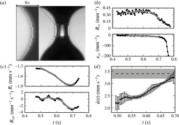
(a) A Newtonian silicone oil filament ( $\unicode[STIX]{x1D707}=1.0~\text{Pa}~\text{s}$ ) in a CBR experiment 600 ms before breakup. The edge detection scheme applied within a domain that excludes the reservoirs results in a piecewise constant description of the free surface (white). A sixth-order least-squares polynomial (black, zoomed in view) applied to the detected edge yields subpixel resolution. (b) The least-squares fits in space are still noisy in time (black), as shown here for $R_{zz}$ and $\unicode[STIX]{x1D705}_{zz}$ evaluated at the filament waist. Results are processed with a triangular centre-weighted running average (grey) to minimize the temporal fluctuations. (c) Temporal derivatives, $R_{t}$ and $R_{zzt}$ , are determined from a running least-squares fit in time (grey). This approach is comparable but less noisy than time derivatives determined by a central differencing scheme (black). (d) Ensemble-averaged surface tension to viscosity ratios $\bar{\unicode[STIX]{x1D6FC}}(t)$ determined by the differential analysis (2.3). Error bars represent the standard error of five replicate trials. The reference value $\unicode[STIX]{x1D6FC}_{ref}$ and its uncertainty are represented by the dashed black line and the grey band, respectively. The results reach the expected value at late times due to filament asymmetry and is discussed in § 6.

The evolving fluid filaments are backlit with a fibre optic lightsource and captured by a Phantom v210 high-speed camera (Vision Research, $1280\times 800~\text{pixels}$ ) through a microscope objective to increase the spatial resolution, particularly in the radial direction. Increasing the magnification limits the field of view and, consequently, the entire free surface profile is not visible, especially before and during the stretching process. Frame rates vary from 40 fps for the most viscous silicone oil to 1000 fps for the least viscous oil. A  $10\times$ Nikon microscope objective (numerical aperture $NA=0.30$ , magnification $M=14,1.2~\unicode[STIX]{x03BC}\text{m}~\text{pixel}^{-1}$ ) aids $R_{p}=2~\text{mm}$ experiments while a 4 $\times$ Nikon objective ( $NA=0.13$ , $M=4.4$ , $3.2~\unicode[STIX]{x03BC}\text{m}~\text{pixel}^{-1}$ ) is used for $R_{p}=3~\text{mm}$ and 4 mm experiments. The step-strain procedure is performed at least five times for each $\unicode[STIX]{x1D707}$ , $R_{p}$ and $L_{f}/L_{0}$ case.

4 Image and data analysis

Images of the filament evolution are analysed in MATLAB^® to determine $R(z)$ at each time step. The time evolution of the filament is traced by an edge detection scheme (Canny Reference Canny1986). The distance between the right and left edges of the free surface (indicated in white in figure 1 a) defines the local value of $2R(z)$ , relatively independent of the filament orientation with respect to the camera frame. The resolution of the edge detection scheme is one pixel, and results in a piecewise constant description of the free surface as shown in the enlarged view in figure 1(a). A polynomial least-squares fit in space is applied to describe the filament radius $R(z)=\sum _{n=0}^{N}R_{n}z^{n}$ at each time step. A fourth-order polynomial fit is the lowest-order fit required to measure $R_{zzzz}$ with a least-squares regression approach. We apply a sixth-order polynomial fit ( $N=6$ ) because we consider a larger domain size to address limitations in the radial spatial resolution. The domain size for these experiments is 20 % of the final separation length $L_{f}$ . The domain avoids the reservoirs and is centred about the waist by requiring the lowest-order odd coefficient in the polynomial fit of $R(z)$ be 0. This constraint ensures the analysis is at a minimum (or maximum) of $R$ . The coefficients of the higher-order odd terms are measures of filament asymmetry about the waist. A non-inertial coordinate system moves with $R_{z}=0$ to achieve local symmetry after an asymmetric stretching process. The coordinate system acceleration is 10 % or less of the gravitational acceleration $g$ . We investigated the effect of a non-inertial coordinate system by performing an alternative experiment where the top plate is raised instead of dropping the bottom plate. The values of $\unicode[STIX]{x1D6FC}$ determined by either (2.3) or (1.4) for either experimental alternative differ by less than 3 %, indicating that the effects of inertia and a non-inertial coordinate are negligible. We also observed that the filament radius in both alternative experiments are larger near the bottom plate (as in figure 1 a). If gravity were negligible, the filament would be fuller near the stationary plate due to inertia. Hence our observations show that gravity is the main source of axial asymmetry. The local Bond number, $Bo(t)=4\unicode[STIX]{x1D70C}gR(0,t)^{2}/\unicode[STIX]{x1D70E}$ , quantifies gravitational effects and decreases as the filament evolves towards breakup ( $R(0,t)\rightarrow 0$ ). Gravitational effects are considered negligible when $Bo(t)<0.1$ (McKinley & Tripathi Reference Mckinley and Tripathi2000).

Time-varying spatial derivatives of $R$ required for (2.3) are determined from derivatives of the polynomial least-squares fit. The least-squares approach suppresses noise due to spatial discretization of the imaged free surface profile, as seen in figure 1(a) for a Newtonian silicone oil filament ( $\unicode[STIX]{x1D707}=1.0~\text{Pa}~\text{s}$ ) in a CBR experiment at $R_{p}=3~\text{ mm}$ and $L_{f}/L_{0}=3$ . However, the least-squares results for $R$ , its spatial derivatives, and consequently $\unicode[STIX]{x1D705}_{zz}$ , evaluated at the filament are still noisy, as illustrated by the black curves for $R_{zz}$ and $\unicode[STIX]{x1D705}_{zz}$ in figure 1(b). A triangular centre-weighted running average (typically 15 points) is applied to $R$ and its derivatives to reduce temporal fluctuations introduced by the time series of least-squares fits in space (grey curves in figure 1 b). The uncertainties in $R$ , its spatial derivatives, and $\unicode[STIX]{x1D705}_{zz}$ are determined by propagating the standard error on the least-squares coefficients. Temporal derivatives, $R_{t}(t)$ and $R_{zzt}(t)$ , are then determined from derivatives of a running least-squares fit in time also applied to 15 points from the triangular centre-weighted results for $R(t)$ and $R_{zz}(t)$ . As seen in figure 1(c), a local temporal least-squares fit (grey curves) produces comparable but less noisy results than a central differencing scheme (black curves). The uncertainties in the time derivatives are determined from the standard error in the temporal least-squares coefficients. The spatial and temporal derivatives of $R$ determine $\unicode[STIX]{x1D6FC}(t)$ by the differential method (2.3) for each trial. Finally, five replicate trials are ensemble averaged for each experimental condition to determine $\bar{\unicode[STIX]{x1D6FC}}(t)$ (figure 1 d). We also determine values of $\unicode[STIX]{x1D6FC}(t)$ by (1.4) with a time-varying necking rate $R_{t}(t)$ , then average over five replicate trials to determine $\bar{\unicode[STIX]{x1D6FC}}(t)$ . The uncertainties in $\bar{\unicode[STIX]{x1D6FC}}(t)$ are the standard error of five trials.

The uncertainties for all terms in (2.3) are monitored, particularly for $R_{zzzz}(t)$ , which has the largest error. Measurements are discarded when the signal-to-noise ratio (SNR) for $R_{zzzz}(t)$ drops below unity, usually close to breakup. An individual trial is discarded when the SNR for $R_{zzzz}(t)$ is less than unity for all time.

The accuracy and errors for terms in (2.3), and subsequently in $\unicode[STIX]{x1D6FC}(t)$ , are sensitive to the least-squares domain size. A sufficiently large domain is desirable to achieve subpixel resolution for the interpolated profile by fitting a relatively low-order polynomial (sixth-order) to hundreds of data points. However, the domain must be sufficiently small to be a local analysis for (2.3). The domain size was varied between $0.15L_{f}$ and $0.25L_{f}$ to minimize errors in $\unicode[STIX]{x1D6FC}(t)$ . Errors in $\unicode[STIX]{x1D6FC}(t)$ can be greater than 20 % for domains smaller than $0.2L_{f}$ because of inadequate radial dynamic range. The selected domain size is $0.2L_{f}$ because it is the domain that minimizes errors in $\unicode[STIX]{x1D6FC}(t)$ near breakup (as $Bo(t)\rightarrow 0$ or $R(0,t)\rightarrow 0$ ).

We evaluated three sets of increasingly unfocused (blurry) image sequences to determine the impact of image sharpness on the detection and fit of the interface. Unfocused image sequences are created by applying a Gaussian filter to the image sequence from one experimental trial. Increasingly unfocused image sequences are obtained by increasing the standard deviation of the filter ( $\unicode[STIX]{x1D70E}_{gauss}=1,3,5$ ). Values of $\unicode[STIX]{x1D6FC}$ determined from these out-of-focus image sequences differ from the original determination by less than 3 % for all $\unicode[STIX]{x1D70E}_{gauss}$ . The outcome of this sensitivity analysis indicates that our technique is robust to imperfect images.

5 Numerical model

We simulate the evolution of a viscous Newtonian fluid filament by numerically solving the 1D model, (1.2) and (2.1), with Runge–Kutta fourth-order temporal integration and a second-order central finite difference scheme on a spatial mesh. The mesh size for the 1D model results shown in figure 2 is 513 nodes. The scales for (1.2) and (2.1) are $R_{p}$ , $\unicode[STIX]{x1D70E}$ and $\unicode[STIX]{x1D707}$ . The scaled bulk continuity equation is the same as (1.2) and the scaled axial momentum equation is

(5.1) $$\begin{eqnarray}(3w_{z}R^{2})_{z}-\unicode[STIX]{x1D705}_{z}R^{2}-BoR^{2}=Re(w_{t}+ww_{z})R^{2},\end{eqnarray}$$

where $Bo=\unicode[STIX]{x1D70C}gR_{p}^{2}/\unicode[STIX]{x1D70E}$ is the Bond number and $Re=\unicode[STIX]{x1D70C}\unicode[STIX]{x1D70E}R_{p}/\unicode[STIX]{x1D707}^{2}$ is the Reynolds number.

Figure 2.

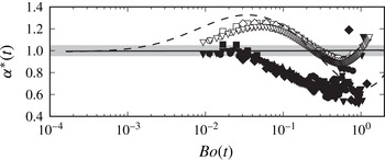
Experimental results for dimensionless surface tension to viscosity ratios $\unicode[STIX]{x1D6FC}^{\ast }(t)$ for five Newtonian silicone oils ( $\unicode[STIX]{x1D707}=0.35~\text{Pa}~\text{s}$ : ●,  $\unicode[STIX]{x1D707}=0.51~\text{Pa}~\text{s}$ : ▪,  $\unicode[STIX]{x1D707}=1.0~\text{Pa}~\text{s}$ : ▴,  $\unicode[STIX]{x1D707}=4.8~\text{Pa}~\text{s}$ : ♦,  $\unicode[STIX]{x1D707}=10~\text{Pa}~\text{s}$ : ▾) versus the local Bond number, $Bo(t)$ . Differential method results (2.3) and standard integral method results (1.4) are shown in filled and open markers, respectively. Every third data point is plotted for clarity. Results determined by applying (2.3) and (1.4) to the 1D model data for a symmetric filament are shown by solid and dashed lines, respectively, with the solid line appearing as $\unicode[STIX]{x1D6FC}^{\ast }=1$ to graphical accuracy. Error bars are not shown for clarity. The grey band indicates the expected value, $\unicode[STIX]{x1D6FC}^{\ast }=1$ , and its error.

The differential analysis (2.3) requires symmetry about the filament waist, as is the case when gravity and inertia are negligible. Thus, we consider the case when $Re=0$ and $Bo=0$ . The initial condition for $R(z)$ at $t=t_{1}$ , when the stretching process ends, is a symmetric, sixth-order polynomial constructed to have the same mass as an initially squat circular fluid cylinder with an initial aspect ratio $\unicode[STIX]{x1D6EC}_{0}=0.733$ and with a final strain $L_{f}/L_{0}=3$ . The axial domain ranges from $-L_{f}/2R_{p}\leqslant z\leqslant L_{f}/2R_{p}$ . The interface remains pinned to the plate edges, represented by $R(z=-L_{f}/2R_{p},t)=R(z=L_{f}/2R_{p},t)=1$ . The no-slip condition at the plates is $w(z=-L_{f}/2R_{p},t)=w(z=L_{f}/2R_{p},t)=0$ . The inertia-free limit of equations (1.2) and (5.1) contain only an evolution equation for $R(z)$ . Therefore, the numerical procedure is as follows: for every $R(z)$ , the corresponding $w(z)$ is solved from (5.1) and then $R(z)$ for the next time step is determined. The dimensionless time step is $\unicode[STIX]{x0394}t=10^{-4}$ . The simulation is halted when $R(0)/R_{p}=0.003$ .

We determine spatial and temporal derivatives of $R$ from the numerical data according to the same procedures for the experimental results (c.f. § 4). These spatial and temporal derivatives are combined to determine dimensionless surface tension to viscosity ratios $\unicode[STIX]{x1D6FC}^{\ast }(t)$ by (2.3). Values of $\unicode[STIX]{x1D6FC}^{\ast }(t)$ for the standard integral method (1.4) are evaluated by the necking rate determined from the 1D model.

We considered two additional symmetric initial conditions for $R(z)$ , including the lubrication solution in Spiegelberg et al. (Reference Spiegelberg, Ables and Mckinley1996). All initial conditions have the same mass as an initially squat fluid cylinder with $\unicode[STIX]{x1D6EC}_{0}=0.733$ and $L_{f}/L_{0}=3$ . The three initial conditions yield similar results for $\unicode[STIX]{x1D6FC}(t)$ determined by (2.3) and (1.4). This indicates (2.3) and (1.4) are insensitive to the initial conditions when the filament is symmetric.

6 Results and discussion

We experimentally evaluate the differential method (2.3) and the standard integral method (1.4) with five Newtonian silicone oils ( $0.35~\text{Pa}~\text{s}<\unicode[STIX]{x1D707}<10~\text{Pa}~\text{s}$ ). We also evaluate (2.3) and (1.4) with numerical data from a preliminary 1D model for an evolving symmetric filament. The 1D model with a symmetric initial condition and negligible gravity and inertia satisfies axial symmetry about the filament waist, as required by (2.3). The initial and final aspect ratios in the 1D model are consistent with the experiments. The performances of (2.3) and (1.4) are compared in figure 2 where the scaled time-dependent surface tension to viscosity ratio $\unicode[STIX]{x1D6FC}^{\ast }(t)\equiv \bar{\unicode[STIX]{x1D6FC}}(t)/\unicode[STIX]{x1D6FC}_{ref}$ is plotted versus $Bo(t)$ . The reference values $\unicode[STIX]{x1D6FC}_{ref}$ are determined by independent measurements of surface tension $\unicode[STIX]{x1D70E}$ and viscosity $\unicode[STIX]{x1D707}$ at $20\,^{\circ }\text{C}$ (§ 3). The uncertainties in $\unicode[STIX]{x1D6FC}_{ref}$ are determined by the errors in independent measurements of $\unicode[STIX]{x1D70E}$ and $\unicode[STIX]{x1D707}$ . The uncertainties in the experimental $\unicode[STIX]{x1D6FC}^{\ast }(t)$ are determined from the standard error in $\bar{\unicode[STIX]{x1D6FC}}(t)$ . Finally, the uncertainty in the expected value, $\unicode[STIX]{x1D6FC}^{\ast }=1$ , is $\pm 5\,\%$ and is determined from the error in $\unicode[STIX]{x1D6FC}_{ref}$ .

The results in figure 2 are plotted against $Bo(t)$ to facilitate comparisons with McKinley & Tripathi (Reference Mckinley and Tripathi2000). The $Bo(t)$ is experimentally relevant because gravity makes the filament profile asymmetric, violating a required assumption for (2.3). Non-negligible gravitational effects are also problematic for (1.4) because it disrupts the assumption that $F$ is constant in space. However, $Bo(t)$ is not suitable for the 1D model because gravity is not considered in either the development of (2.3) or (1.4). Even so, we present the 1D model results as a function of $Bo(t)$ determined by $g=9.81~\text{m}~\text{s}^{-2}$ (instead of $g=0$ ) to compare with experimental results. We discuss alternate approaches to rescaling our problem below.

In figure 2, the experimental results determined by (2.3) are scattered and noisy shortly after the stretch ( $Bo(t)>0.3$ ). The scatter and noise decrease as $Bo(t)$ decreases until $Bo(t)<0.2$ , when the results become independent of the viscosity range considered. The differential method results for $\unicode[STIX]{x1D6FC}^{\ast }(t)$ are 30–40 % below the expected value of unity for $Bo(t)<0.2$ , but approach unity as $Bo(t)$ further decreases, reaching the expected value for $Bo(t)<0.04$ . Uncertainties in $\unicode[STIX]{x1D6FC}^{\ast }(t)$ for $Bo(t)<0.3$ are typically less than $10\,\%$ . The result evaluated by applying (2.3) to the 1D model data is constant with $Bo(t)$ and deviates less than 0.5 % from $\unicode[STIX]{x1D6FC}^{\ast }=1$ . The result for $\unicode[STIX]{x1D6FC}^{\ast }$ using the 1D model data is essentially error free because the 1D model and (2.3) share the same assumptions (axial symmetry about the waist, rectilinear flow, gravity- and inertia-free). Deviations in the experimental results from $\unicode[STIX]{x1D6FC}^{\ast }=1$ may also be caused by small viscoelastic and surfactant effects in the silicone oils that are not captured by the 1D model or (2.3). However, the deviations from $\unicode[STIX]{x1D6FC}^{\ast }=1$ are caused by filament asymmetry in the CBR experiments, as discussed below.

The experimental differential method results presented here are determined by (2.3) without the inertial terms. The results for $\unicode[STIX]{x1D6FC}^{\ast }(t)$ change the largest- $Re$ silicone oil ( $\unicode[STIX]{x1D707}=0.35~\text{Pa}~\text{s}$ ) by less than 5 % and only near breakup ( $Bo(t)<0.04$ ) when such inertial terms are included. Therefore, inertial effects are small for the test fluids considered in this study and are not considered in (2.3) for the rest of this paper.

The experimental results determined by (1.4) in figure 2 overlap for all $Bo(t)$ shown and indicate that this method is independent of $\unicode[STIX]{x1D707}$ within the range tested. As $Bo(t)$ decreases, $\unicode[STIX]{x1D6FC}^{\ast }(t)$ first grows to a maximum then decreases again towards but does not reach unity. The 3 % uncertainties in the experimental results determined by (1.4) are smaller than the 10 % uncertainties in (2.3). The larger uncertainties in the differential method results stem from measurements of higher-order derivatives of $R(z,t)$ (discussed in figure 1). The result determined by applying (1.4) to the 1D model data when $Bo(t)>0.0005$ follows a similar trend as the experimental results. However, $\unicode[STIX]{x1D6FC}^{\ast }(t)$ determined from the 1D model data has larger deviations from $\unicode[STIX]{x1D6FC}^{\ast }=1$ than the experimental results. Furthermore, the minimum and maximum values predicted from the 1D model are shifted horizontally relative to the experimental results.

The differences between the experimental and 1D model results are related to gravitational effects on the necking rate $R_{t}(t)$ , because the experiments are subjected to gravity while the 1D model results are not. These differences suggest that gravity increases $|R_{t}|$ at early times but decreases $|R_{t}|$ at longer times. Our findings are consistent with the numerical results with and without gravity in McKinley & Tripathi (Reference Mckinley and Tripathi2000). The variation in $\unicode[STIX]{x1D6FC}^{\ast }(t)$ throughout earlier times, corresponding to high $Bo(t)$ , in the filament evolution is due to force and curvature approximations. It also shows that $|R_{t}|$ is not constant and that a time-dependent correction factor is required in this regime. The 1D model result for $\unicode[STIX]{x1D6FC}^{\ast }$ determined by (1.4) reaches a constant value of unity for $Bo(t)<0.0005$ . This indicates that the filament waist evolution does follow the similarity solution of Papageorgiou (Reference Papageorgiou1995) when $Bo(t)<0.0005$ , because applying $X=0.7127$ in (1.4) yields the correct result.

McKinley & Tripathi (Reference Mckinley and Tripathi2000) recommends that (1.4) be applied when $Bo(t)<0.1$ . However, experimental and 1D model results determined by (1.4) in figure 2 show that a smaller, stricter $Bo(t)$ criterion is necessary to improve the accuracy of measurements performed at the sample volume and strain conditions studied here. As mentioned by McKinley & Tripathi (Reference Mckinley and Tripathi2000), the time required to reach the self-similar regime described by Papageorgiou (Reference Papageorgiou1995) depends on multiple parameters, including sample volume and strain. Therefore the $Bo(t)$ criterion to indicate when the filament evolution has reached the self-similar regime will also vary with sample volume and strain. For the conditions considered here, which correspond to those studied by McKinley & Tripathi (Reference Mckinley and Tripathi2000), the $Bo(t)$ criterion needs to be much stricter than $Bo(t)<0.1$ .

In addition to varying $\unicode[STIX]{x1D707}$ , we experimentally investigate the operating range of the differential method (2.3) with three sample volumes, represented by plate radius $R_{p}=2$ , $3$ and $4~\text{mm}$ , and three strains, $L_{f}/L_{0}=2$ , 3 and 4.5. The largest strain case has the flattest (least curved) filament profile, indicated by small $R_{zz}$ and $R_{zzzz}$ . Despite our use of microscope objectives to resolve the filament, the profile for the largest strain case typically varies by less than 10 pixels in the radial direction. The radial variation in all other filament profiles are resolved with 2 to 4 times as many pixels. The SNR for $R_{zzzz}(t)$ is below unity throughout the $L_{f}/L_{0}=4.5$ trials; therefore, this condition has been excluded from our analysis.

The time-dependent experimental differential method results for varying $\unicode[STIX]{x1D707}$ , $R_{p}$ , and $L_{f}/L_{0}$ are summarized in figure 3. The results are plotted as a function of two different time-varying parameters to determine a suitable dimensionless variable to characterize the filament evolution: $Bo(t)$ and dimensionless radius at the waist scaled by the local free surface curvature, $R_{zz}$ . Time increases from right to left in each of the plots in figure 3. The results for all experimental conditions shown have large deviations from $\unicode[STIX]{x1D6FC}^{\ast }=1$ at early times, corresponding to large dimensionless parameter values. The results generally approach and reach $\unicode[STIX]{x1D6FC}^{\ast }=1$ as the dimensionless parameters decrease corresponding to late times. The only exception is the smallest strain case, which increases to $\unicode[STIX]{x1D6FC}^{\ast }=0.85$ . The results plotted against $Bo(t)$ generally collapse while $\unicode[STIX]{x1D6FC}^{\ast }(RR_{zz})$ do not when the sample volume or strain are varied. A universal curve is not expected for $\unicode[STIX]{x1D6FC}^{\ast }(RR_{zz})$ , because $R_{zz}(t)$ is affected by sample volume and strain.

Dimensionless CBR results are commonly presented according to time non-dimensionalized by a visco-capillary or inertio-capillary time scale, $R(t)/R_{p}$ , and $Bo(t)$ (Papageorgiou Reference Papageorgiou1995; McKinley & Tripathi Reference Mckinley and Tripathi2000; Anna & McKinley Reference Anna and Mckinley2001; Bhat et al. Reference Bhat, Appathurai, Harris, Pasquali, Mckinley and Basaran2010). A dimensionless time is problematic because it requires an arbitrarily defined reference time such as the time at breakup or the time when the plates come to rest. In addition, $R(t)/R_{p}$ is not suitable because (2.3) and (1.4) are local analyses and $R_{p}$ is an external dimension relevant to the reservoir and not the fluid filament. Scaling the radius at the waist with a local length scale such as $R_{zz}(t)$ , the free surface curvature at the waist, is a more meaningful approach to represent dimensionless radius in our local analysis (2.3). But the lack of a universal curve for $\unicode[STIX]{x1D6FC}^{\ast }(RR_{zz})$ (shown in figure 3 b) makes it difficult to develop a criterion to indicate when to apply (2.3) based on this parameter. For practical purposes we therefore suggest a criterion based on $Bo(t)$ to indicate when the differential method (2.3) is valid. Theoretically $Bo(t)$ is not a relevant parameter because gravity is neglected in the differential method (2.3) to enforce axial symmetry and ultimately avoid an axial fluid velocity measurement at the waist. Gravity (and inertia) is also neglected in (1.4) to avoid a spatially varying axial force. Even when gravitational effects are included, (2.3) is not explicit in $g$ because it does not appear in the differentiated equations after being evaluated at the filament waist. Instead the effect of gravity is detected in the filament shape because it disrupts the axial symmetry required by (2.3).

Figure 3.

Experimental results for dimensionless surface tension to viscosity ratios $\unicode[STIX]{x1D6FC}^{\ast }(t)$ determined by (2.3) plotted against two dimensionless time-dependent parameters. Results are shown for five Newtonian silicone oils ( $\unicode[STIX]{x1D707}=0.35~\text{Pa}~\text{s}$ : ●,  $\unicode[STIX]{x1D707}=0.51~\text{Pa}~\text{s}$ : ▪,  $\unicode[STIX]{x1D707}=1.0~\text{Pa}~\text{s}$ : ▴,  $\unicode[STIX]{x1D707}=4.8~\text{Pa}~\text{s}$ : ♦,  $\unicode[STIX]{x1D707}=10~\text{Pa}~\text{s}$ : ▾), three sample volumes ( $R_{p}=2~\text{ mm}$ : 

,  $R_{p}=3~\text{mm}$ : ▴,  $R_{p}=4~\text{mm}$ : 

), and two strains ( $L_{f}/L_{0}=2$ : 

,  $L_{f}/L_{0}=3$ : ▴). Error bars are the standard error of five replicated trials. Every second data point is shown for clarity and error bars are shown for every fourth point. The grey band indicates the expected value, $\unicode[STIX]{x1D6FC}^{\ast }$ = 1, and its error.

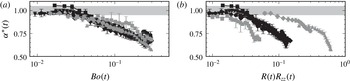
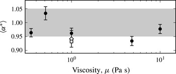
Figure 3(a) shows that differential method results are accurate for $Bo(t)<0.04$ . The experimental results are summarized in figure 4, where time-averaged differential method results $\langle \unicode[STIX]{x1D6FC}^{\ast }\rangle$ are plotted against viscosity $\unicode[STIX]{x1D707}$ ; except for the $L_{f}/L_{0}=2$ case, because the series terminates early owing to limited temporal resolution. The results in figure 4 are determined by averaging all values of $\unicode[STIX]{x1D6FC}^{\ast }(t)$ for $Bo(t)<0.04$ . The uncertainties in $\langle \unicode[STIX]{x1D6FC}^{\ast }\rangle$ are one standard deviation for values of $\unicode[STIX]{x1D6FC}^{\ast }(t)$ when $Bo(t)<0.04$ .

Values of $\langle \unicode[STIX]{x1D6FC}^{\ast }\rangle$ determined by (2.3) for the five Newtonian silicone oils agree with the expected value. These time-averaged results are relatively constant with respect to viscosity, and are independent of sample volume (with an outlier at $R_{p}=4~\text{mm}$ ). Uncertainties in $\langle \unicode[STIX]{x1D6FC}^{\ast }\rangle$ for all cases in figure 4 are less than 4 %.

Figures 2 and 3 indicate the appropriate range to analyse differential method results is at late times corresponding to $Bo(t)<0.04$ . We examine the assumptions made in deriving (2.3) to identify the cause for deviations from $\unicode[STIX]{x1D6FC}^{\ast }=1$ at earlier times (larger $Bo(t)$ ). The symmetry condition required by (2.3) is mainly disrupted by gravitational effects (larger sample volumes) for the experimental conditions investigated here. When the filament is asymmetric, two additional terms requiring a velocity measurement at the waist, $wR_{zzz}/\unicode[STIX]{x1D705}_{zz}R$ and $ww_{zz}/6\unicode[STIX]{x1D708}\unicode[STIX]{x1D705}_{zz}$ , would need to be included in (2.3) to determine $\unicode[STIX]{x1D6FC}$ . To maintain a purely geometric approach, we measure the asymmetry about the waist to determine when the two additional terms may be considered negligible. We define an asymmetry measure

(6.1) $$\begin{eqnarray}\unicode[STIX]{x1D6FA}(t)=\frac{\left|R_{zzz}(t)\right|}{R_{zz}^{2}(t)+\left|R_{zzzz}(t)\right|^{2/3}}.\end{eqnarray}$$

This definition compares the relative magnitudes of $R_{zzz}(t)$ , a measure of filament asymmetry about the waist, to the gradients of curvature that drive the filament evolution.

Figure 4.

Experimental results for time-averaged dimensionless surface tension to viscosity ratios $\langle \unicode[STIX]{x1D6FC}^{\ast }\rangle$ determined by the differential method (2.3) versus viscosity, $\unicode[STIX]{x1D707}$ . Results are shown for five Newtonian silicone oils ( $0.35~\text{Pa}~\text{s}<\unicode[STIX]{x1D707}<10~\text{Pa}~\text{s}$ : ●) and three sample volumes ( $R_{p}=2~\text{mm}$ : ♢,  $R_{p}=3~\text{mm}$ : ●,  $R_{p}=4~\text{ mm}$ : ▫). Results are determined by averaging over $Bo(t)<0.04$ and error bars represent one standard deviation. The $L_{f}/L_{0}$ = 2 result does not generate a time-averaged value because the data set does not extend past $Bo(t)<0.04$ . The grey band indicates the expected value, $\unicode[STIX]{x1D6FC}^{\ast }=1$ , and its error.

The differential method results for $\unicode[STIX]{x1D6FC}^{\ast }(t)$ versus asymmetry $\unicode[STIX]{x1D6FA}(t)$ for varying $\unicode[STIX]{x1D707}$ , $R_{p}$ and $L_{f}/L_{0}$ are plotted in figure 5 for $Bo(t)<0.3$ . Excluded results for larger $Bo(t)$ are noisy, with uncertainties greater than 10 % (see figure 2). Values of $\unicode[STIX]{x1D6FC}^{\ast }(t)$ generally follow the same behaviour. At short times, $\unicode[STIX]{x1D6FA}(t)$ increases towards its maximum and $\unicode[STIX]{x1D6FC}^{\ast }$ is underestimated, typically by 30 %. For the viscosity range considered, $\unicode[STIX]{x1D6FC}^{\ast }(t)$ grows gradually as $\unicode[STIX]{x1D6FA}(t)$ approaches its maximum. In contrast, $\unicode[STIX]{x1D6FA}(t)$ grows gradually compared to the increase in $\unicode[STIX]{x1D6FC}^{\ast }(t)$ for $R_{p}=2~\text{mm}$ and $L_{f}/L_{0}=2$ . Unlike other results, $\unicode[STIX]{x1D6FA}(t)$ generally decreases when $Bo(t)<0.3$ for the $R_{p}=4~\text{ mm}$ case.

The differential method results approach $\unicode[STIX]{x1D6FC}^{\ast }=1$ from below as asymmetry decreases. Generally, $\unicode[STIX]{x1D6FC}^{\ast }(t)$ reaches unity near breakup $(Bo(t)<0.04)$ as $\unicode[STIX]{x1D6FA}(t)$ rapidly decreases, with the exception of noisy $\unicode[STIX]{x1D6FC}^{\ast }(t)$ , when asymmetry becomes small. In addition, the overall asymmetry decreases with growing $R_{p}$ despite our expectations that a larger sample volume would have greater asymmetry, especially before stretching. The errors in $\unicode[STIX]{x1D6FC}^{\ast }(t)$ also grow with increasing $R_{p}$ . This behaviour indicates that measurements for the larger samples are more challenging because of smaller axial curvatures caused by larger gravitational effects. Methods to reduce noise in measuring $R$ and its derivatives are part of continuing work.

Figure 5.

Experimental results for dimensionless surface tension to viscosity ratios $\unicode[STIX]{x1D6FC}^{\ast }(t)$ determined by (2.3) versus asymmetry $\unicode[STIX]{x1D6FA}(t)$ for $Bo(t)<0.3$ . Results are shown for five Newtonian silicone oils ( $\unicode[STIX]{x1D707}=0.35~\text{Pa}~\text{s}$ : ●,  $\unicode[STIX]{x1D707}=0.51~\text{Pa}~\text{s}$ : ▪,  $\unicode[STIX]{x1D707}=1.0~\text{Pa}~\text{s}$ : ▴,  $\unicode[STIX]{x1D707}=4.8~\text{Pa}~\text{s}$ : ♦,  $\unicode[STIX]{x1D707}=10~\text{Pa}~\text{s}$ : ▾), three sample volumes ( $R_{p}=2~\text{mm}$ : 

,  $R_{p}=3~\text{mm}$ : ▴,  $R_{p}=4~\text{ mm}$ : 

), and two strains ( $L_{f}/L_{0}=2$ : 

,  $L_{f}/L_{0}=3$ : ▴). Unfilled markers represent values when $Bo(t)<0.04$ . Error bars are the standard error of five replicated trials and are shown on every 3rd data point for clarity. The grey band indicates the expected value, $\unicode[STIX]{x1D6FC}^{\ast }=1$ , and its error.

Figure 5 shows that axial symmetry is a key requirement to develop a geometric differential analysis (2.3). The negligible error in comparing (2.3) to the 1D symmetric model demonstrates that most of the experimental error is due to asymmetry. Discrepancies in $\unicode[STIX]{x1D6FC}^{\ast }(t)$ determined by (2.3) are attributed to the missing velocity terms that diminish as the asymmetry decreases near breakup.

Figure 5 also shows no universal curve, as expected, for $\unicode[STIX]{x1D6FC}^{\ast }(\unicode[STIX]{x1D6FA})$ because filament asymmetry is affected by the initial Bond number (sample volume) and the strain as well as the initial aspect ratio, initial asymmetry and strain rate. Furthermore, filament asymmetry is indicated by deviations of $R(z)$ and $w(z)$ from purely even and odd functions, respectively, and hence our definition of $\unicode[STIX]{x1D6FA}(t)$ (6.1) is incomplete. All curves in figure 5 demonstrate that the differential analysis (2.3) accurately determines $\unicode[STIX]{x1D6FC}^{\ast }$ when asymmetry is sufficiently small and $\text{d}\unicode[STIX]{x1D6FC}^{\ast }/\text{d}\unicode[STIX]{x1D6FA}\rightarrow 0$ (or $\text{d}\unicode[STIX]{x1D6FC}^{\ast }/\text{d}Bo(t)\rightarrow 0$ ). The asymmetry should be assessed as sufficiently small compared to the initial asymmetry. We are not yet able to evaluate the asymmetry before and during the stretching process because microscope objectives improve radial resolution but limit the field of view. In the future a cylindrical lens will enable measurements of the entire filament evolution while increasing the radial resolution. As a proxy, sufficiently small asymmetry for accurate determination of $\unicode[STIX]{x1D6FC}^{\ast }$ occurs when $Bo(t)<0.04$ and $\text{d}\unicode[STIX]{x1D6FC}^{\ast }/\text{d}Bo(t)\rightarrow 0$ .