2.1 Wing geometry modelling

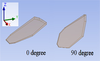
The geometry of the wing used was adopted from the experimental investigation carried out by Rehmat^{(Reference Rehmat12)} and Rehmat et al.^{(Reference Rehmat, Lee, Trabia, Roll and Yim13)} The wing thickness tapers from the base (4mm) to the tip (1mm), as shown in the plan view of the wing in Fig. 1. The spanwise and chordwise location (0, 0) indicates the anchoring point of the wing. The horizontal axis at chordwise 0mm is the rotation axis for the wing, and the pitch angle of the wing is based on this axis; see for example Fig. 2, which shows a 3D view of the wing at 0° and 90° initial pitch angle, $\theta$_{p_initial}. The wing base is located at spanwise 60.55mm, and the wingtip at 188.5mm. The length of the wing is 138mm.

Figure 1.

Plan view of the edges and cross-sections of the proposed wing represented by red, blue, and green lines, where (0, 0) is the centre of rotation and L denotes the length of the wing.

Figure 2.

3D view of the wing at initial pitch angle $\theta$_{p_initial} of 0° and 90°.

2.2 Governing equations for two-way FSI and data analysis

The mass conservation equation for incompressible flow (density = constant) is given as follows:

(1) \begin{equation}\nabla \cdot\vec v =0\end{equation}

where ∇ is divergence and$\;\vec v$ is velocity. The momentum conservation equation is as follows:

(2) \begin{equation}\rho \frac{{\partial \vec v}}{{\partial t}} + \rho \left( {\vec v\cdot\nabla } \right)\vec v = - \nabla p + \mu {\nabla ^2}\vec v + \rho \overrightarrow {{F_x}},\end{equation}

where $\rho$ is density, t is time, p is pressure, $\mu $ is viscosity and F _x represents the external forces. The Shear Stress Transport (SST) k–ω turbulence model was used as compromise between accuracy and computation cost, and this model is recommended in various similar previous studies.^{(Reference Frunzulica, Dumitrache and Stoia-Desjka17,Reference Aftab, Rafie, Razak and Ahmad25–Reference Radermacher27)} The SST k–ω turbulence model transport equations are as follows:

(3) \begin{equation}\frac{\partial }{{\partial t}}\left( {\rho k} \right) + \frac{\partial }{{\partial {X_i}}}\left( {\rho k{u_i}} \right) = \frac{\partial }{{\partial {X_j}}}\left( {{D_k}\frac{{\partial k}}{{\partial {X_j}}}} \right) + {X_k} - {I_k} + {Y_k},\end{equation}

(4) \begin{equation}\frac{\partial }{{\partial t}}\left( {\rho \omega } \right) + \frac{\partial }{{\partial {X_i}}}\left( {\rho \omega {u_i}} \right) = \frac{\partial }{{\partial {X_j}}}\left( {{D_\omega }\frac{{\partial \omega }}{{\partial {X_j}}}} \right) + {X_\omega } - {I_\omega } + {Y_\omega },\end{equation}

where X _k and X _ω are the turbulence kinetic energy and specific rate generation due to the velocity gradient, I _k and I _ω are the k and ω diffusivity and Y _k and Y _ω are external forces.

The stress–strain matrix equation for the structural dynamics is as follows:

(5) \begin{equation}\lfloor{\sigma _x}{\sigma _y}{\sigma _z}{\sigma _{xy}}{\sigma _{yz}}{\sigma _{xz}}\rfloor^T = \left[ S \right]\left\{ {{b^v}} \right\}\end{equation}

where σ _n is the stress vector (n=x, y, z, xy, yz, xz), S is the elasticity, and b is the elastic strain vector.

The equations used for the data analysis are presented below. The normalisation of the results in this study was based on the following equation:

(6) \begin{equation}{R_{norm}} = \frac{{{R_{org}} - {R_{min}}}}{{{R_{max}} - {R_{min}}}},\end{equation}

where R _norm is the normalised data, R _org is the original data, R _max is the maximum value of the data and R _min is the minimum value of the data. The lift coefficient C _L is defined as

(7) \begin{equation}{C_L} = \frac{{{F_L}}}{{0.5\rho S{{\left( {{U_{tip\_max}}} \right)}^2}}}\end{equation}

where F _L is the lift force, $\rho$ is the density of air, S is the wing area and U _{tip_max} is the maximum wingtip velocity. The Reynolds number Re of the wing undergoing figure-of-eight motion is calculated using the following equations based on refs. (Reference Hope, DeLuca and O’Hara28) and (Reference Bhat, Zhao, Sheridan, Hourigan and Thompson29), respectively:

(8) \begin{equation}{\rm{Re}} = \frac{{4\rho \left( {2{\theta _s}} \right)fhR}}{{\mu {A_R}}}\end{equation}

(9) \begin{equation}{A_R} = \frac{h}{\bar{c}}\end{equation}

where $\theta$_s is the stroke angle as defined in section 2.3, f is the frequency, R is the length measured from the (0, 0) anchoring point to the wingtip referred to in section 2.1, μ is the dynamic viscosity of air, A _R is the wing aspect ratio, h is the wingspan and $\bar{c}$ is the average wing chord length, which is the ratio of the wing area to the wingspan. The maximum Reynolds numbers is 25,391, 38,086 and 50,781, respectively, for input link angles of 30°, 45°, and 60°.

2.3 Input and boundary conditions

We consider a 3D domain with height, width and length of 40cm, 30cm and 50cm, respectively, as shown in Fig. 3, which illustrates the outlines of the wing and the fluid domain and highlights the boundary conditions applied at the inlet, outlet and walls. The position of the centre of rotation of the wing is located at 10cm offset from the centre of the fluid domain towards the negative X-axis direction. The inlet value is set to 0m/s due to the hovering motion of the wing, which does not induce any free-stream velocity against itself. The outlet is set to the default pressure outlet. The figure-of-eight motion for the wing model in the CFD simulations is based on the formulations and mechanism described by Duffy^{(Reference Duffy and Roth30)} and Rehmat et al.^{(Reference Rehmat, Lee, Trabia, Roll and Yim13)} Briefly, the spherical four-link mechanism and the angles between each link are translated into spherical trigonometry. The base of the wing is set to move in three different directions, described using the stroke angle $\theta$_s, heave angle $\theta$_h and pitch angle $\theta$_p. The change in the angles over a flapping cycle are converted into angular speeds, and these values are provided as boundary inputs to the wing. Figure 4a illustrates the stroke $\theta$_s, heave $\theta$_h, and pitch $\theta$_p, angles of the wing for an initial pitch angle of $\theta$_{p_initial} = 0°, while Fig. 4b–d shows the stroke, heave and pitch angles and angular speed per cycle. The maximum velocity of the wing tip is 7.253m/s, 10.258m/s and 21.729m/s for the input link angles of 30°, 45°, and 60°. These maximum velocities for the wing tip were calculated based on the angular speeds as shown in Fig. 4b–d. Figure 5a shows the wing tip trajectories for input link angles of 30°, 45°, and 60°; Basically, the use of a higher input link angle increases the spatial size of the figure-of-eight motion. Figure 5a and b shows the change of the pitch angle of the wing (cross-sectional view at 75% L of the wing) over the cycle, namely from 1/16 to 16/16, for the case with $\theta$_{p_initial} = 0° and 90°, respectively.

Figure 3.

Fluid domain and wing outlines showing the inlet (yellow), outlet (green) and wall (white) boundary conditions. The centre of rotation of the wing is marked with an “x,” while the centre of the fluid domain is marked with an “o.”

Figure 4.

(a) Illustration of the stroke ($\theta$_s), heave ($\theta$_h) and pitch ($\theta$_p) angles of the wing with an initial pitch angle of $\theta$_{p_initial} = 0°. The stroke ($\theta$_s), heave ($\theta$_h) and pitch ($\theta$_p) angles and the angular speed are shown for one cycle for input link angles of (b) 30°, (c) 45° and (d) 60°.

Figure 5.

(a) Wingtip trajectories for input link angles of 30°, 45° and 60° at 75% L wing section from cycles 1/16 to 16/16 viewed along the negative x-axis for $\theta$_{p_initial} values of (b) 0° and (c) 90°.

The fluid is stagnant at the initial condition as there is no wing motion. The properties of air, such as the density and kinematic viscosity, are considered to be constant, being obtained from the work of McCormick^{(Reference McCormick31)} at 15°C. The wing material is set to balsa wood to allow benchmarking against a condition similar to the experimental work of Rehmat.^{(Reference Rehmat12)} The detailed properties of dry balsa wood, e.g., the Young’s moduli along the three axes, the density, the Poisson’s ratio, the flexural strength, and the compressive strength, were obtained from Forest Products Laboratory, USDA⁽³²⁾ (Table 1). Based on the wood grain properties shown in the wing prototype surface of Rehmat^{(Reference Rehmat12)} and Rehmat et al.,^{(Reference Rehmat, Lee, Trabia, Roll and Yim13)} it is assumed that model-grade balsa wood sheet was a tangent cut, so the longitudinal Young’s modulus is set spanwise (with the wood grain direction parallel to the span) while the radial and tangential Young’s moduli are set along the chordwise and flapwise direction, respectively.

Table 1

Properties of wing and air

2.4 Numerical method

The solver used in the numerical analysis of this study is based on unsteady simulations together with dynamic mesh features. The FSI model in Ansys–Fluent commercial software^{(Reference Fluent33)} is used in this study. The model is based on two-way system coupling between the fluid and structural parts. For the pressure–velocity coupling, the pressure-implicit with splitting of operators (PISO) scheme is used.^{(Reference Sohail and Ullah34,Reference Wan and Huang35)} For comparison, we also tested the coupled pressure–velocity scheme, finding no significant difference. The pressure field is solved by using the second-order discretisation scheme, while the momentum is solved by the second-order upwind scheme. The least-squares cell-based method is applied in the spatial discretisation schemes. First-order upwind schemes are used to discretise the turbulent kinetic energy and specific dissipation rate. The Courant–Friedrichs–Lewy (CFL) condition is set to be lower than unity using the equation

(10) \begin{equation}{C_n} = \frac{{{V_a}\Delta t}}{{\Delta x}} < 1\end{equation}

where C _n represents the Courant number, V _a is the velocity magnitude, Δt is the time step and Δx is the mesh node interval. A constant time step of 5 × 10⁻⁴s is used. Residual values of 10⁻⁴ is set as the convergence criterion.

2.5 Simulation cases

There are two main types of simulation cases. In the first type, the initial pitch angle of the wing $\theta$_{p_initial} is varied from 0° to 360° in steps of 30°; For these cases, the input link angle is fixed at 45°. For the second type, three different input link angles are compared, i.e., 30, 45° and 60°, for $\theta$_{p_initial} = 0° and 90°. The rotation speed in all cases is 12.25Hz (4.89s per cycle). For validation and benchmarking, the results from our CFD case with $\theta$_{p_initial} = 0° and input link angle of 45° are compared with a similar experimental investigation by Rehmat.^{(Reference Rehmat12)}

2.6 Meshing, grid-independence test and validation

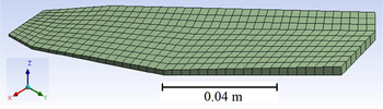
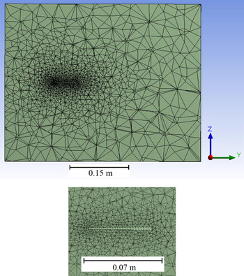
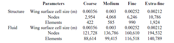
The ANSYS meshing module was used for the meshing process. The mesh cell shape for the fluid domain is tetrahedral, while prisms were adopted in the structural mesh domain. Inflation layers were not generated due to the complex figure-of-eight motion, as the inclusion of such layers would require a long time for remeshing the fluid domain, thereby increasing the computational time tremendously. The high cell aspect ratio of the inflation layers would also favour divergence of the solution, thus increasing the probability of negative cell volumes during remeshing. Despite the lack of prism layers, the average dimensionless wall distance was kept at y ⁺ < 5. A wing surface y ⁺ below 5 is acceptable to resolve the boundary layer according to the Fluent user guide.^{(Reference Fluent33)} To reveal the effect of mesh refinement and the magnitude of the error on the predicted results, a grid independence test and solver validation were conducted. Figures 6 and 7 show the intermediately refined meshing for the fluid and structural domains. The mesh properties of the fluid and structural mesh domain are presented in Table 2. The authors acknowledge the importance of adding prism layers at the boundary to predict the viscous layer near the wing surface. However, given the complex nature of the flapping motion (figure of eight), which consists of rotations, heave and flapping motions, together with the limited computational power available, the current numerical code cannot be run with the prism layers preserved during the dynamic meshing of the flapping motion. This is due to the deficiency of the available dynamic meshing scheme that can be used to preserve the mentioned prism layers at large simulation time steps. Under this condition, the authors can only apply one mesh cell type, which is tetrahedral, to ensure the optimal mesh quality of the FSI simulations throughout all the time steps. However, to strengthen the reliability of the results presented herein, the current mesh is further refined by setting the wing surface cell size to extra fine (0.00212m). The results presented in the next section show that there are no significant differences in the results obtained using the extra-fine versus fine mesh, thus indicating that the fine mesh is adequate for this study.

Figure 6.

Intermediate refinement meshing for the wing in the transient structural solver.

Figure 7.

Intermediate refinement mesh slice of the fluid domain.

Table 2

Coarse, medium, fine and extra-fine mesh properties

The “dynamic meshes” setting of the transient structural solver includes the implementation of the fluid–solid interface on the surface meshes of the wing and also turning on the “large deflection” feature, which predicts the stiffness variation due to deformation. To preserve the quality of the fluid domain meshes throughout the simulation period, the Laplace smoothing and local cell remeshing methods were adopted. In the Laplace smoothing settings, a spring constant factor of 1, a convergence tolerance of 0.001, 20 iterations, and a Laplace node relaxation of 1 are defined. In the local cell remeshing settings, the default minimum and maximum length scale of the tetrahedral domain meshes are based on the smallest and largest mesh sizes of the fluid domain, and the maximum cell skewness is set to 0.7. The system coupling function is set in Fluent, which allows the transfer of force and displacement data between the transient mechanical solver and the Fluent solver through the mentioned fluid–solid interfaces. Therefore, no user-defined function (UDF) is required to enable the dynamic mesh motion.