Introduction
Practitioners conducting on-farm and exploratory industrial studies often use factorial designs with properly replicated treatments to ensure the precision of estimated treatment effects (Laurent et al., Reference Laurent, Miguez, Kyveryga and Makowski2020). These trials typically evaluate farmers’ practices by comparing emerging technologies or management methods with a range of established practices. For example, a study may investigate two factors – soil treatment and lime incorporation method, each including newly developed techniques whose effects on crop yield require direct evaluation against numerous traditional methods. The new techniques are of explicit interest and are therefore considered fixed, whereas the traditional practices represent a larger population of existing approaches and are more appropriately treated as random. In addition, the current yield may be influenced by prior management practices or soil treatments – a phenomenon referred to as pre-history effects – making it important to account for these legacy influences to accurately estimate the effects of the new techniques. Such experiments lead to treatment factors that simultaneously contain fixed and random levels, highlighting the need for analytical methods capable of handling this structure while accounting for pre-history effects. Benefits from developed technologies should be well articulated to convince farmers to abandon their traditional farming systems in favour of the new technologies. Use of statistical models that accommodate both fixed and random levels for each factor of interest offers essential flexibility while achieving the desired efficiency.
Njuho and Milliken (Reference Njuho and Milliken2005, Reference Njuho and Milliken2009) motivated this approach with an example on weeding methods where new crop varieties are introduced to communities that grow traditional varieties. The interest in that setting would be to investigate the effects of variety and weeding method as factors on crop yield, with the newly introduced varieties and weeding methods of particular interest, hence, considered as fixed factor levels. By contrast, given the full range of traditional varieties or weeding methods that is not exhaustively known, a random sample of them is drawn for each factor. The new treatments are then compared to the mean of the sample of existing treatments in current use. The mean of the existing treatments is modelled as a further fixed level of each factor, whereas variation of these treatments around the mean is modelled by random effects. Implementing this model is not possible when we consider the traditional approach of defining a factor as either fully fixed or as fully random, a practice that continues to generate a hot debate amongst researchers (Borenstein et al., Reference Borenstein, Hedges, Higgins and Rothstein2009; Huang, Reference Huang2020; Kanters, Reference Kanters, Evangelou and Veroniki2022; Koretz, Reference Koretz2022; Leyland, Reference Leyland2010; Payne and Loadsman, Reference Payne and Loadsman2024; Ryoo, Reference Ryoo2011). Instead, a combination of fixed and random factor levels is required.
The proposed approach finds its applicability in different fields of science and technology such as agriculture and industrial studies (Chaka and Njuho, Reference Chaka and Njuho2022; Njuho and Milliken, Reference Njuho and Milliken2005). For example, technologies with promising results may undergo evaluation in on-farm trials to incorporate the farmers’ practices, environmental and management conditions. The process ensures that the developed technologies meet efficiency and sustainability requirements. The conception of formalized on-farm trial programmes and the use of high-profile precision technologies make it easier to conduct on-farm trials (Licht and Witt, Reference Licht and Witt2019) and to compare performance of a new technology to existing ones under various farming conditions (Saito et al., Reference Saito, Diack, Dieng and N.’Diaye2015).
Usually, the aforementioned experiments are conducted to compare the effectiveness of new against traditional production techniques (Thu et al., Reference Thu, Thuong and Minh2022), to make informed decisions, improve production practices, optimize resource allocation, and enhance overall productivity. To obtain useful information about the effect of the tested production practices on the response variable and its uncertainty in such studies, appropriate statistical analysis approaches are needed (Piepho et al., Reference Piepho, Williams and Fleck2006). With increasing interest in on-farm precision experimentation, the use of state-of-art precision technology to inexpensively run large-scale agronomic field trials (Bullock et al., Reference Bullock, Mieno and Hwang2020; Kyveryga, Reference Kyveryga2019; Tanaka, Reference Tanaka2021), there is a pressing need to develop rigorous statistical methods for evaluating the efficacy of new equipment, management strategies and technologies under specified conditions with all the inherent variation present in a specific production system (Johnston et al., Reference Johnston, Renteria-Flores and Hannon2003; Rakshit et al., Reference Rakshit, Baddeley, Stefanova, Reeves, Chen, Cao, Evans and Gibberd2020).
Njuho and Milliken (Reference Njuho and Milliken2005, Reference Njuho and Milliken2009) established that some factorial experimental designs are more efficient when some factors are conceptualized as comprising some levels that are fixed and others that are random. In particular, when testing a set of new treatments, these would be assigned fixed treatment levels, whereas established treatments would be assigned a common mean and random levels for deviations from that mean so that the new treatments can be compared to the population of established treatments. Ultimately, the fixed levels allow for comparison of specific levels, while the random levels assist in assessing the amount of variability within a subset of the factor levels considered as a benchmark.
Traditionally, capturing of fixed and random levels of factors often involves partitioning of the response data into subsets based on the targeted factor levels and the research objectives before conducting a separate partitioned analysis (Chaka and Njuho, Reference Chaka and Njuho2021, Reference Chaka and Njuho2022). The manual process of syncretizing the degrees of freedom and sum of squares from the partitioned analysis is the basic approach of obtaining a combined analysis for such experiments (Njuho and Milliken, Reference Njuho and Milliken2005). Nevertheless, researchers are often tempted to shoehorn the traditional approach that considers a factor as either fixed or random in a distinct form, thereby compromising the accuracy of the analysis. Either way, linear mixed models are preferred because they account for data variability under the assumptions made on both the covariance structure and the mixture models. It is, therefore, crucial to identify and select an appropriate experimental design as well as a suitable model to avoid misleading inferences (Bate and Chatfield, Reference Bate and Chatfield2016).
Previous studies by Chaka and Njuho (Reference Chaka and Njuho2021, Reference Chaka and Njuho2022) focused on partitioned analyses that evaluated selected factor levels independently, providing insights into individual treatment comparisons. However, their approach does not integrate information across all factor levels, nor does it account for potential pre-history effects arising from prior management practices. This limitation defines the critical gap addressed in the present study: the need for a framework that generates combined analyses, incorporating all factor-level effects within a single linear mixed-model structure. Such an approach enables simultaneous evaluation of new and traditional practices while explicitly accounting for pre-history effects, thereby providing a more comprehensive and robust assessment of treatment impacts on the response variable. Combining analyses of variance from partitioned linear models is particularly challenging when factors include both fixed and random levels, with complexity increasing for large sample sizes or more than two factors. To address these challenges, the current study proposes a unified mixed-model procedure for analysing all factors simultaneously, building on concepts of efficient experimental designs for comparative experiments as reviewed by Piepho (Reference Piepho2015) and implemented using SAS PROC GLIMMIX or CRAN-based software.
The goal of this study is to propose a structured framework for modelling experimental designs that include factors with both fixed and random levels. It is hypothesized that this approach provides a coherent and practically applicable linear mixed-model formulation that supports integrated analysis across factor levels while accounting for pre-history effects of prior management practices. The specific objectives are to develop the model for a single-factor case and extend it to multi-factor designs.
Materials and methods
Data
Crop yield data simulated from an on-farm trial, conducted at a site in Bute, Northern Yorke Peninsula of South Australia in 2019–2022, where barley, lentil and wheat have been continuously grown for many years in rotation (Trengove et al., Reference Trengove, Sherriff, Bruce, Noack and Hughes2023) was used to illustrate the applicability of the proposed approach. The experimental site consisted of a paddock with a red sandy topsoil layer over sandy clay soil with low levels of organic carbon (0.5 %), low cation exchange capacity, low salinity and different soil acidity (pH levels) at different levels of surface soil. These Bute soil properties were analysed in 5 cm-depth increments ranging from 0–30 cm, as well as 30–60 cm and 60–100 cm depths since the soil samples collected initially included these segments (Trengove et al., Reference Trengove, Sherriff, Bruce, Noack and Hughes2023).
Slow movement of surface applied lime, reported as little as 1 – 2.5 cm per year (Burns et al., Reference Burns, Norton and Tyndall2017; Fleming et al., Reference Fleming, Fraser, Dohle and Hughes2020), requires appropriate incorporation and mixing techniques to accelerate its movement in the soil. Depending on the type of machinery and different depths required, various options of lime incorporation methods can be considered. These lime incorporation techniques include cultivation, deep ripping with or without inclusion plates, spading and combinations of these (Trengove et al., Reference Trengove, Sherriff, Bruce and Noack2021). To effectively manage the soil pH and to keep it within the preferred range of 6–8.5 for improving crop productivity (Hughes, Reference Hughes2020), investigations on the effectiveness of these incorporation techniques and soil treatments for a particular crop on a given type of soil, are necessary. For this example, the effect of the following factors on the yield of barley was considered, while assuming that all other factors remain unchanged or fixed:
-
Soil treatment – with six (6) levels, i.e., nil (control group), sulphur, and four (4) sources of lime (Kulpara, Angaston, Spalding and Venning).
-
Lime/sulphur incorporation method – with seven (7) levels, i.e., no till, offset disc, deep ripping, inclusion ripping, spading, a combination of offset disc + inclusion, and a combination of offset disc + inclusion + spade.
The methodology is illustrated through three increasingly complex and practically relevant examples: a completely randomized design analysing the effects of soil treatment and lime/sulphur incorporation method on barley yield; a repeated-measures design analysing the effects of soil treatment and lime/sulphur incorporation method on normalized difference vegetation index (NDVI), observed at four time points in cereal and lentil plants; and a split–split-plot design under a completely randomized layout, analysing the effects of irrigation method, irrigation treatment, and wheat cultivar on wheat yield. Together, these examples demonstrate how the proposed approach can be applied in practice to a broad class of experimental designs frequently encountered in agricultural and biological research.
Methods
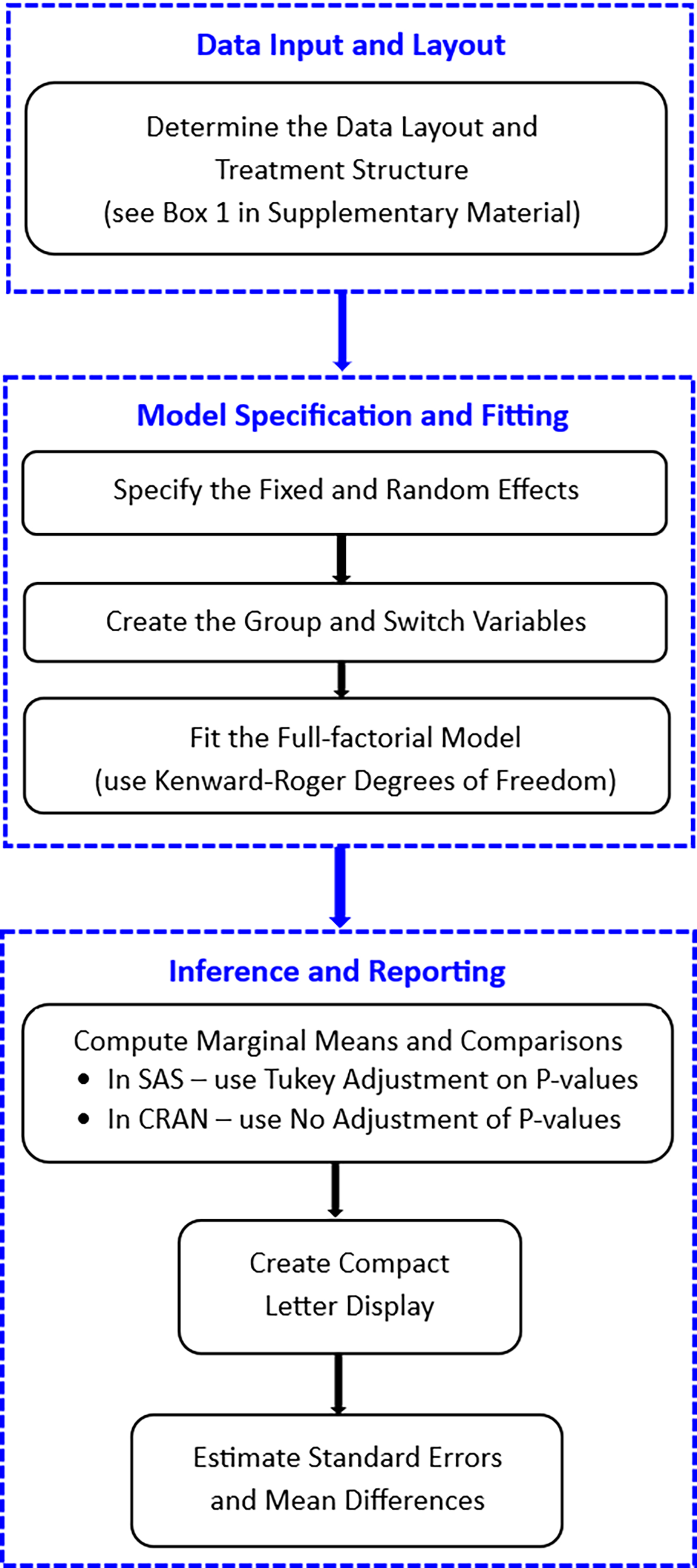
Figure 1 illustrates the stepwise analysis process, from data preparation and specification of treatment structure, through model fitting and computation of marginal means – including options for P value adjustment (Tukey adjustment in SAS; no adjustment in CRAN) – to the generation of pairwise comparisons and reporting of results.
Workflow of the statistical analysis.

The case of a single factor
Suppose that a single factor consists of r random levels selected from a population of old and existing levels, and f new (fixed) levels, whose effects on the response variable need to be tested. The analysis of such a treatment structure is not a straightforward case (Piepho et al., Reference Piepho, Williams and Fleck2006) and, therefore, a careful selection of an appropriate linear model that provides a meaningful analysis of variance to be formulated.
Model construction
Suppose a single factor (e.g., soil treatment) has r a random levels, representing a random sample of soil treatment methods chosen from a population of traditional soil treatment methods; and f a fixed levels, representing new soil treatment methods, whose effects on crop yield (y) are to be tested. The experiment allows m replicates for each treatment. The model for the fixed-effect part (purposefully manipulated soil treatment levels) of the data is given by
 ${y_{F_{ij}}}= {\mu_F} + {\alpha_i^F} + {\epsilon_{ij}^F}, (i=1,\ldots,f_a),$
where yFij
is the response of the j
th
replication (j = 1,…,m) receiving the i
th
treatment (i = 1, …, f
a
), μ
F
is the overall mean,
 ${ {\alpha_{i}^F}}$
is the i
th
fixed effect of the factor, and effects
 ${ {\epsilon_{ij}^F}}$
are independent and identically distributed (i.i.d.) random error terms, with
 ${ {\epsilon_{ij}^F}} \sim i.i.d{\,\,}{N(0; {\sigma_{\epsilon^F}^2})}$
.
Similarly, the model of the random-effect part of the data is given by
 ${y_{R_{ij}}} = \mu_R + \alpha_i^R + \epsilon_{ij}^R, (i = {f_a} + 1,\;{f_a} + 2, \ldots, {f_a} + {r_a}),$
where y
R
ij
is the response of the j
th
replication (j = 1,…,m) receiving the i
th
treatment (i = f
a
+ 1, f
a
+ 2, …, f
a
+ r
a
), μ
R
is the overall mean,
 ${ {\alpha_{i}^R}} \sim i.i.d{\,\,}{N(0; {\sigma_{\alpha}^2})}$
is the random effect of the treatment factor, and
 ${ {\epsilon_{ij}^R}} \sim i.i.d{\,\,}{N(0; {\sigma_{\epsilon^R}^2})}$
are residual errors.
For illustration purposes, consider an experiment involving a single factor, with six levels, A1 through A6, where four (A1 – A4) are considered as random (i.e., r a = 4) and two levels (A5 and A6) are considered as fixed (i.e., f a = 2), with three replications per treatment (i.e., m = 3). The first step in the analysis process is to create two new variables, ‘group’ and ‘switch’, that will be used to identify and combine the fixed and random levels of the factor in the dataset. Supplementary Box 1 displays the combined data layout of this experiment, with the ‘group’ variable whose levels are constituted by the fixed levels (coded as ‘A5’ and ‘A6’) and a set of all the random levels of the factor combined (coded as ‘random’), and the numerical ‘switch’ variable (0,1) set to zero for the fixed levels and to one for the random levels.
For the combined data the mixed nature of the factor requires a joint model that can be written as (Piepho et al., Reference Piepho, Williams and Fleck2006)
 $y_{ij}=\mu +\gamma _{g(i)}+z_{g(i)}\alpha _{i}+\epsilon _{ij}, (g(i)=1,\ldots, f_{a},f_{a}+1),$
where y
ij
is the response of the j
th
replication (j = 1,…, m
i
) in the g(i)-th group of levels of the factor (i = 1,2, …, f
a
, f
a
+ 1), μ is the overall mean, g(i) is the group to which treatment i is assigned, where each fixed level i corresponds to a separate group (g(i) = 1 to f
a
), and all the random levels i are collected into a single group g(i) = f
a
+ 1, γ
g(i) is the fixed effect of the g(i)-th group for i = 1,2, …, f
a
and
 ${\gamma _{g( \,{{f_a} + 1} )}}$
is a random effect group, and z
g(i)
α
i
, where the switch variable z
g(i) = 0 for i = 1 to f
a
, and z
g(i) = 1 for i = f
a
+ 1 to f
a
+ r
a
, is the i
th
random effect in the g(i)-th group of levels of the treatment factor. Note that the fixed effects of the joint model (3) can be related to those of the separate models (1) and (2) via the equations μ
F
+ α
i
= μ + γ
g(i) for i = 1 to f
a
and μ
R
= μ + γ
f
a
+ 1.
To explain the effect of the switch variable z
g(i) in the random-effects part of the joint model, let Z be the design matrix for a single factor of interest and assume initially that all levels are random. Then if G is the corresponding variance-covariance matrix, the contribution to the variance-covariance matrix of the data is ZGZ
T
. Now if some of the levels of the factor are fixed, we need to set the corresponding entries in ZGZ
T
to zero. This can be done in two different ways. The first one is to set all elements to zero in columns of Z corresponding to fixed levels of the factor. This may be implemented by fitting a random effect, factor.switch, where switch = 0 in all records for fixed levels of the factor and switch = 1 for all random levels of the factor. The second option is to remove columns comprising only zeros from Z and reduce the dimension of G accordingly. To see that both options are equivalent, let Z be partitioned as
 $Z=(Z_{f}\, Z_{r})$
and G as G = G
f
⊕ G
r
, where the symbol ⊕ represents the direct sum operator, Z
f
and G
f
pertain to the fixed levels of the factor, and Z
r
and G
r
to the random levels. The first option replaces Z
f
with 0, yielding
 $\left( {\matrix{ 0 & {{Z_r}} \cr } } \right)\left( {{G_f} \oplus {G_r}} \right)\left( {\matrix{ {{0^T}} \cr {Z_r^T} \cr } } \right) = {Z_r}{G_r}Z_r^T$
. The second option reduces Z to Z
r
and G to G
r
, yielding the same contribution
 ${Z_r}{G_r}{Z_r^T}$
to the variance-covariance matrix of the data. Hence, both implementations are equivalent and yield the same residual likelihood. The first option is implemented in our SAS and R codes given in the Supplementary Material.
Alternative notation for a single treatment factor
Partitioned analysis based on a subset of the data and the targeted fixed or random levels of the factor provides a concentrated analysis on similar treatment levels. However, it is generally preferable to use all data, i.e. all factor levels, to obtain a more powerful analysis than a subset of the data. A fit to the whole data allows for all comparisons of interest to be derived. To achieve this, we introduce an alternative notation to express model (3) in a more convenient way. Let z g(i) be represented by a numeric variable ‘switch’, and the group levels g(i) be represented by a factor ‘group’. The treatment levels i are represented by ‘factor’. Then, the right-hand side of model (3) can be stated as
 $group\; + \;group.factor.switch,$
with ‘group’ coding the fixed group effect γ g(i), and the term ‘group.factor.switch’ coding the random treatment effect z g(i) α i . The SAS and R codes for fitting a full linear model for a single factor are displayed in Supplementary Boxes 2(a) and (b), respectively.
Factorial treatment with multiple factors
An alternative representation to illustrate the full-factorial model when multiple factors are involved is introduced. The concept is illustrated using two factors (A and B), noting that it is easily extended to any multi-factor scenario. For compactness of model statements, let each factor be represented by a single letter (say, factorA = A), the grouping factor by ‘g’ and a letter defining the factor (say, groupB = gB), and the numeric switch variable by ‘s’ and a letter defining the factor (say, switchB = sB). The factorial model is obtained by crossing the two single-factor models defined in model (4) using the operator ‘×’ to represent the crossing of factors or models (Piepho et al., Reference Piepho, Büchse and Emrich2003; Wilkinson and Rogers, Reference Wilkinson and Rogers1973):
 $\begin{align}(gA &+ gA.A.sA) \times (gB + gB.B.sB) = gA + gA.A.sA + gB\cr & + gB.B.sB +gA.gB + gA.gB.B.sB + gB.gA.A.sA \cr & + gA.A.sA.gB.B.sB\cr\end{align}$
The effects involving only gA and/or gB are fixed, while all other effects are random. Hence, the fixed effects in model (5) are: gA + gB + gA.gB.
To illustrate the concept further, consider an investigation conducted on a single response variable that is predicted by two categorical factors A and B. Suppose that factor A has four random levels, r a1 through r a4, and two fixed levels, f a5 and f a6; factor B has five random levels, r b1 through r b5, and three fixed levels, f b6, f b7 and f b8. The basic layout of the data for this factorial study with five replications per treatment, is displayed in Supplementary Box 3. Similar to the single-factor case, the ‘group’ and ‘switch’ variables are created for the two factors for easy reference. Supplementary Boxes 4(a) and 4(b) illustrate the syntaxes for creating these variables in the SAS and CRAN R environments, respectively.
The code creates additional ‘gA’ and ‘gB’ variables in the original dataset, that specify the groups of fixed and random levels in the respective factors, where the random levels are combined into one group level that is designated as ‘random’ while the fixed levels are stored in their individual categories. In addition, the code creates the numerical ‘sA’ and ‘sB’ variables that specify the random (coded as 1) and fixed (coded as 0) levels whose effects are to be estimated in the fitted model.
The combined model is built from all the factor(s) levels (both random and fixed) in the study. Using the dataset (Data2groups) created in the previous step (see Supplementary Boxes 4(a) and (b)), the SAS PROC GLIMMIX and R procedures for fitting the combined models using Kenward-Roger degrees of freedom are illustrated in Supplementary Boxes 5(a) and (b), respectively. It is crucial to ensure proper settings are used to specify the intended model. For example, the control settings function in R provides the flexibility of controlling convergence issues in the fitted model.
This paper is focused on the null hypothesis that a new treatment equals the mean of the population of old treatments, citing several relevant use cases. In practice, it may also be important to formally test the null hypothesis that the new treatment effect arises from the same distribution as the existing treatments, which were modelled as random effects. In other words, one should assess whether the new treatment comes from the same population as the old treatments (i.e., the treatment-specific means in that population have a constant variance). While this test would provide insight into whether the new treatment is consistent with the established population of treatments or represents a deviation, it falls outside the scope of the current paper. Existing approaches to such hypothesis testing (e.g., Francq et al., Reference Francq, Lin and Hoyer2019; Sharma and Mathew, Reference Sharma and Mathew2012; Oliva-Avilés and Hauser, Reference Oliva-Aviles and Hauser2025) are often limited by restrictive assumptions on the linear mixed model structure, particularly the requirement that variance components enter linearly in the variance-covariance structure. This excludes commonly encountered correlation structures such as AR(1) as considered in our second example.
Results
The applicability of the proposed approach is illustrated across different experimental designs, namely a completely randomized design (CRD), a repeated measures design, and a split-split-plot design.
A case of a completely randomized design
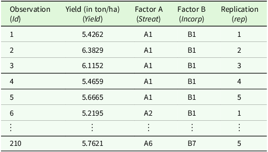
To illustrate the proposed approach, consider a case of two factors (A – soil treatment, and B -incorporation technique), each having both fixed and the random levels, used to predict a single response variable (barley yield, in tons per hectare (t/ha)). Suppose that the treatments are designed in a CRD, where the two factors are: A (with four random levels, r a1 through r a4, and two fixed levels, f a1 and f a2); and B (with four random levels, r b1 r b2,r b3 and r b5, and three fixed levels, f b4, f b6 and f b7). Let factor A be soil treatment (Streat), with six levels (A1 – control, A2 – sulphur, A3 – Kulpara, A4 – Angaston, A5 – Spalding and A6 – Venning), where a random sample of four (4) traditional lime products (A1, A2, A3, and A4) are to be tested against two new lime products (A5 and A6) taken as fixed soil treatment levels. Let lime/sulphur incorporation method (Incorp) be factor B with seven levels (B1 – no till, B2 – offset disc, B3 – deep ripping, B4 – inclusion ripping, B5 – spading, B6 – offset disc + inclusion, and B7 – offset disc + inclusion + spade), where a random sample of four incorporation methods (B1, B2, B3 and B5) were to be tested against three newly suggested methods (B4, B6 and B7) taken as fixed levels. A two-way CRD, with five replications per treatment was proposed for the experiment. A sample size of 210 is considered sufficient for this experiment (Hair et al., Reference Hair, Black, Babin and Anderson2019). Table 1 shows the design of the simulated data from the Bute on-farm experiment (see Supplementary Figure 1 and Note 2).
Barley yield data simulation design

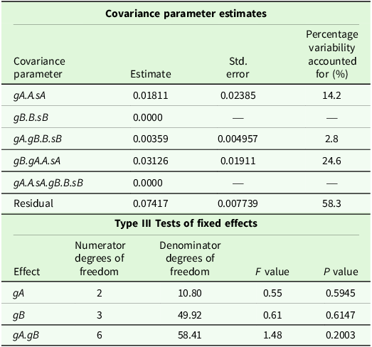
Assume that the interest of the study is to estimate and compare the effects of the new farming strategies (fixed effects) against the means of the old and existing ones (random effects), the combined analysis of variance in these two sets is appropriate. The SAS and R syntax given in Supplementary Boxes 5(a) and (b) were used to obtain the combined analysis for this experiment. Table 2 summarizes the analysis of variance for the combined model.
Combined ANOVA for the barley on-farm experiment

Note: A represents factor A, gA represents group A, and sA represents switch A. Corresponding notation is used for factors B and C (i.e., B, gB, sB and C, gC, sC).
In this experiment, the interaction of these farming methods (gA.gB) was not statistically significant at a significance level of α = 0.05 (P value = 0.2003). The same applies to the main effects of newly suggested soil treatment methods (gA) and the new lime/sulphur incorporation methods (gB), indicating that these new farming techniques were not sufficiently contributing to the variation in the barley yield. The combined analysis provides a broader perspective of the effects of all the factors (fixed or random) on the response variable in the experiment. The last column of the first section of Table 2 shows the percentage total variability accounted for by each random effect. Much of the total variation in the barley yield is attributed to the traditional (random levels) of soil treatment (gA.A.sA) products (14.2%), and the interaction of these traditional soil treatment products and the traditional lime incorporation methods (gA.A.sA.gB.B.sB) (24.6%).
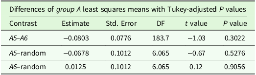
A comparison of the marginal means was considered since the interaction of the treatment effects (gA.gB) was not significant in the barley yield experiment. That is, the means of factor A averaged across factor B, and the B means averaged across A. Multiple comparisons of treatment means were conducted and reported using the ‘insert-and-absorb’ algorithm guaranteed to always truthfully represent all significant differences (Piepho, Reference Piepho2004) that is implemented in the SAS % mult macro (Piepho, Reference Piepho2012) and the ‘multcompView’ package in R. Supplementary Boxes 6(a) and (b) show the SAS and R procedures for generating the mean comparisons and letter display. However, it requires that the % mult macro code be submitted first, and then the simplified SAS code in Supplementary Boxes 5(a) and 6(a) would produce the results in Tables 2 and 3. Tables 3 and 4 display part of the associated output that includes the letter display, with the significant differences in the mean yield of barley at the α = 0.05 level.
Pairwise comparisons for marginal means of group A (Tukey-adjusted)

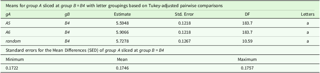
Mean comparisons, letter display (Tukey-adjusted) and variability statistics of group A sliced by group B: Part of the output for group B = B4

Note: gA represents group A; A5 and A6 represent fixed levels of factor A; while random represents the set of all random levels associated with factor A. Analogous notation is used for factor B.
The mean comparisons reported in the main text were obtained using either Tukey-adjustment for P values in SAS glimmix or unadjusted (t tests) P values in R multiview. Table 3 displays the pairwise comparisons of marginal means of group A based on the Kenward–Roger method for calculating the degrees of freedom and the Tukey method for the adjustment of P values. The differences between the three marginal mean estimates are not significant (P values > 0.05). Table 4 displays the adjusted mean for each group level combination (group A sliced at group B = B4) along with associated standard errors and letter display. All three groups (A5-B4, A6-B4, random-B4) share the same letter ‘a’, implying no significant differences between the adjusted means of these groups. In addition, the values of the Standard Error of Difference (SED) were relatively stable (range = 0.1722 to 0.1757, mean = 0.1746), providing a reliable and consistent estimate of the precision of mean comparisons.
A case of repeated-measures design
A three-factor repeated-measures experiment is considered, with two between-subject factors – factor A (with six levels) and factor B (with seven levels) – and one repeated-measures (within-subjects) time factor (Time) with three time points with six replications per treatment, to test for significant differences in the response variable. The experiment assumes a CRD where the experimental units (plots, in this case) were randomly assigned to the levels of factor A and factor B with no blocking or stratification. The Bute on-farm experiment (Trengove et al., Reference Trengove, Sherriff, Bruce, Noack and Hughes2023) measured and monitored the greenness and health of cereal and lentil plants in four consecutive seasons using the NDVI, a numerical index derived from remote sensing satellite imagery. A higher NDVI value indicates healthier and denser vegetation. The proposed approach is illustrated using simulated NDVI values for the four trial seasons of 2020, 2021, 2022 and 2023, predicted by soil treatment (factor A) and lime incorporation method (factor B) where factors A and B are conceptualized as each having both fixed and random levels, and the levels of the repeated-measures time factor (in years) are considered as fixed (see Supplementary Note 3). The repeated-measures linear mixed model is given in the alternative notation as
 $\eqalign{ \left( {gA\;} \right. & \left. {+ \;gA.A.sA} \right) \times \;\left( {gB\; + \;gB.B.sB} \right) \times Time = gA\; + \;gB\; \cr & + gA.gB + Time + \;\;Time.gA + Time.gB + Time.gA.gB \cr & + gA.A.sA\; + \;gB.\;gA.A.sA\; + gA.A.sA.gB.B.sB \cr & + Time.gA.A.sA + gB.B.sB + gA.gB.B.sB + Time.gB.B.sB \cr & + Time.gA.gB.B.sB + Time.gB.\;gA.A.sA \cr & + Time.gA.A.sA.gB.B.sB,\; \cr}$
where the effects involving only gA, gB, Time, or interactions among these factors are fixed, while the rest are random. Hence, the fixed effects in model (6) are:
gA + gB + gA.gB + Time + Time.gA + Time.gB + Time.gA.gB.
Analogous to the previous example, we consider the combined analysis of variance based on all the fixed and random effects in the experiment. The focus is on investigating the effects of two between-subject factors: soil treatment (factor A), with four random levels (A1 – A4) and two fixed levels (A5 and A6); lime incorporation method (factor B), with four random levels (B1, B2, B3, and B5) and three fixed levels (B4, B6 and B7); and a single within-subjects time factor C with three fixed levels; on the NDVI response variable. The variation in the response variable (purposefully simulated for illustration), observed over the four trial seasons was modelled using a linear mixed-effects model in a repeated-measures design (RMD) with six replications per treatment. The RMD assumed that the treatments (combinations of factors A and B) are arranged in a CRD with the first order autoregressive [AR(1)] error variance-covariance structure with an independent nugget effect. First, the data for a repeated-measures experiment needs to be captured and laid out in univariate format, as displayed in Supplementary Box 7.
Once the data layout is correctly done, the fixed and random levels of each factor are defined and set into appropriate categories. The syntax used to set the data into the convenient (univariate) format, and to create the ‘group’ and ‘switch’ variables is displayed in Supplementary Boxes 8(a) and (b). For this experiment, the levels of the time factor were regarded as fixed, and therefore used as such in the analysis. To investigate and visualize the changes in mean levels of the response variable due to a specific predictor variable over time, the mean NDVI is plotted against time. An example is given for factor B against time, before the full-factorial model is fitted. Supplementary Boxes 9(a) and (b) display the SAS and R codes for generating and visualizing the mean NDVI contribution by factor B over time, as well as the full-factorial repeated-measures model with an autoregressive covariance structure of lag 1, AR(1).
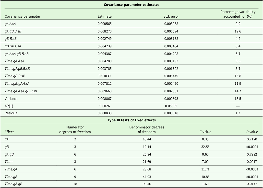
Supplementary Boxes 10(a) and (b) display the SAS and R codes for generating the full factorial repeated-measures model. A summary of the analysis of variance from the full-factorial repeated-measures model is shown in Table 5. Slight discrepancies between the variance components produced in R glmmTMB and SAS proc glimmix packages are attributed to the estimation of an additional residual variance (nugget) in the two procedures. Nonetheless, the residual autocorrelation, AR(1), and most of the random components are relatively similar. Results presented in the main text are based on SAS output. Part of the random effects estimates, and the type III tests for the effects of the fixed levels of factors A, B and time in the fitted model are displayed in Table 5.
ANOVA for the full factorial repeated-measures model

Note: A represents factor A, gA represents group A, sA represents switch A, and Time represents the repeated-measures time factor. Corresponding notation is used for factor B (i.e., B, gB, sB).
The ANOVA results show a nonsignificant effect of the interaction of new levels of the two between-subject factors and time (Time.gA.gB), the interaction of these two factors (gA.gB) and the main effect (gA) as shown by P values greater than 0.05. However, there is a significant interaction (P values < 0.05) of time and fixed levels of both factors A and B (Time.gA and Time.gB) at α = 0.05. Of equal importance are the covariance parameter estimates for the random effects in the model. The last column of the covariance parameter estimates section in Table 5 shows the percentage total variability accounted for by each random effect. About 25.7% (12.6 + 6.4 + 6.7) of the total variation in the NDVI indices is attributed to the interaction of the traditional lime incorporation methods (gB) with the soil treatment methods (gA), and around 54.6% (6.5 + 5.7 + 15.8 + 11.9 + 14.7) of the total variation attributed to the effects of time on these farming methods.
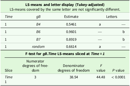
Given that neither Time.gA.gB nor gA.gB is significant, and that gB, Time.gA and Time.gB are significant, we assess and compare the marginal means for Time.gA and Time.gB within each specific time level. The SAS and R codes for generating a comparison of the treatment means are given in Supplementary Boxes 10(a) and (b). Table 6 shows the comparisons of Time.gB means sliced at Time = 1, the letter display and the associated F-test.
Comparisons of means of group B.Time sliced at time = 1

Note: gB represents group B; B4, B6 and B7 represent the fixed levels of factor B; random represents the set of all random levels associated with factor B; and Time represents the repeated-measures time factor.
The results from the first part of Table 6 indicate that, at a significance level of α = 0.05, groups B4 and ‘random’ are not significantly different from each other (LS-means covered by the same letter ‘a’). However, these two groups (B4 and ‘random’) are each significantly different from either B6 or B7 that are both covered by letter ‘b’. In addition, the F-test for the interaction effect of gB.Time within Time = 1, averaged across all levels of gA, is statistically significant (P value < 0.05).
A case of a split-split-plot in a completely randomized design
Owing to recent development in irrigation equipment, farmers have adopted precision irrigation techniques such as pressurized irrigation methods (e.g., drip and sprinkler irrigation) to manage field loss in crop production (Anjum et al., Reference Anjum, Cheema, Hussain, Wu and Zaman2023). Making an appropriate choice between irrigation methods (Jha et al., Reference Jha, Ramatshaba, Wang, Liang, Liu, Gao and Duan2019; Liu et al., Reference Liu, Liu, Huang, Liu, Meng, Chen, Ma and Liu2024; Pan et al., Reference Pan, Wang, Liu, Bao, Chen, Akmalov, De Maeyer and Van de Voorde2023; Yuan et al., Reference Yuan, Tai, Mao, Tam, Li, Wu and Li2023), farmer practices, irrigation and fertigation (applying fertilizers through the irrigation system to maintain soil nutrients levels) practices (Taha and Ouda, Reference Taha and Ouda2016), and crop variety for a particular field are extremely important decisions (Dube et al., Reference Dube, Tsilo, Sosibo and Fanadzo2020; Kong et al., Reference Kong, Li, Peng, Zhang, Hu, Wang and Zhao2023) for improved productivity in irrigated agriculture. Irrigation systems are hard-to-change, and thus, considered as whole-plot factors in the split-split-plot (SSP) experiments. The conventional linear model for a SSP treatment arrangement with the whole-plot factor laid in a CRD (purposefully constructed for the treatment factors only), where each treatment combination is replicated m times, is alternatively expressed as,
 $\eqalign{ \left( {gA\;} \right. & \left. {+ \;gA.A.sA} \right) \times \;\left( {gB\; + \;gB.B.sB} \right) \times \left( {gC\; + \;gC.C.sC} \right) = gA\; \cr & + gB\; + gC\; + gA.gB\; + \;gA.gC + gB.gC + gA.gB.gC \cr & + gA.gB.B.sB + \;gA.A.sA\; + gA.A.sA.gB\; \; + gB.B.sB \cr & + gA.gB.B.sB\; + \;gA.A.sA.gB.B.sB\; + gA.A.sA.gC\; \cr & + \;gA.A.sA.gB.gC\; + \;gB.B.sB.gC\; + gA.gB.sB.gC\; \cr & + gA.A.sA.gB.B.sB.gC\; + \;gC.C.sC\; + \;gA.gC.C.sC\; \cr & + \;gA.A.sA.gC.C.sC + \;gB.gC.C.sC\; + gA.gB.gC.C.sC\; \cr & + \;gA.A.sA.gB.gC.C.sC\; + \;gB.B.sB.gC.C.sC\; \cr & + gA.gB.B.sB.gC.C.sC\; + \;gA.A.sA.gB.B.sB.gC.C.sC,\; \cr}$
where A represents factor A, gA represents group A, sA represents switch A and corresponding notation is used for factors B and C. The fixed effects in the model are:
gA+gB + gC+gA.gB+gA.gC + gB.gC+gA.gB.gC.
For the purpose of illustrating the proposed concept, the proposed model (7) is limited to treatment effects only. The design effects (e.g., whole-plot error, split-plot error and SSP error) could be considered as random effects that determine the structure of the experiment and the estimate of variability. We illustrate our concept using simulated data (see Supplementary Note 4) from on-farm irrigated wheat cultivar trials (Dube et al., Reference Dube, Tsilo, Sosibo and Fanadzo2020), deficit irrigation and fertigation trials (Jia et al., Reference Jia, Dai, Xie and He2021; Taha and Ouda, Reference Taha and Ouda2016), and irrigation techniques (Jamali et al., Reference Jamali, Soufizadeh, Yeganeh and Emam2021; Wang et al., Reference Wang, Gong, Xu, Yu and Zhao2013; Yuan et al., Reference Yuan, Lin, Maucieri and Zhang2022). A SSP treatment structure laid in a CRD, where the effect of whole-plot factor A (irrigation method – with five levels: A1 – drip, A2 – sprinkler, A3 – alternative furrow irrigation, A4 – centre pivot, and A5 – basin), the split-plot factor B (irrigation treatment – with eight levels: B1 – required irrigation at 1.2 ETc (crop evapotranspiration) and fertigation 80 % of time, B2 – required irrigation at 1.2 ETc and fertigation 60 % of time, B3 – deficit irrigation at 1.0 ETc and fertigation 80 % of time, B4 – deficit irrigation at 1.0 ETc and fertigation 60 % of time, B5 – deficit irrigation at 0.8 ETc and fertigation 80 % of time, B6 – deficit irrigation at 0.8 ETc and fertigation 60 % of time, B7 – deficit irrigation at 0.6 ETc and fertigation 80 % of time, B8 – deficit irrigation at 0.6 ETc and fertigation 60 % of time and fertigation 60 % of time, and the SSP factor C (cultivar – with five levels: C1 – SST 8154, C2 – Sabie, C3 – PAN 3515, C4 – Duzi, C5 – Krokodil, and C6 – PAN 3400) on irrigation wheat yield (in t/ha), is considered. Two (2) irrigation methods (A2 and A4), four (4) irrigation treatments (B2, B4, B6 and B8), three (3) wheat cultivars (C1–C3), are considered as new (fixed) recommendations to be tested against the numerous traditional (random) methods. All possible interactions of these factors are allowed. Let a, b and c denote the levels of factor A, B and C, respectively. The data layout for this experiment is similar to the general layout illustrated in Table 1. The SAS and R syntax for deriving all the effects of a three-way model and generating a combined SSP linear mixed-effects model are given in Supplementary Boxes 11(a) and (b), respectively. In most cases, convergence issues are commonly encountered when fitting large linear models such as this. The convergence issues were handled by fitting the model using the PROC HPMIXED procedure to identify the variances that converge to zero, and eliminating these effects before fitting a reduced model using the GLIMMIX procedure. Alternatively, one could use the PROC MIXED procedure since it makes the convergence criterion absolute.
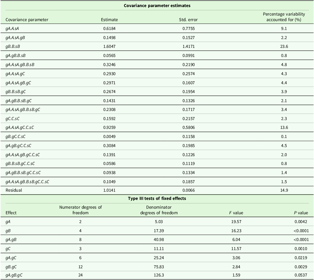
Table 7 displays the random effects and the type III tests of fixed effects of the fitted reduced model, after eliminating some of the random effects with zero variances (rep.A, rep.A.B, and gA.gC.C.sC). The tests of the fixed effects show that the highest-order interaction gA.gB.gC is not significant (P value > 0.05) whereas the all the three lower-order interactions (gA.gB, gA.gC and gB.gC) are significant (P value < 0.05). A non-significant three-way interaction (gA.gB.gC), but one or more significant lower-order interactions (say gA.gB) indicates that the effect of one two-way interaction does not vary depending on the level of the third factor (say gC). Thus, we can consider the mean comparisons of the levels of one factor, say factor B (gB), within each combination of the other two, say A and C (gA.gC).
ANOVA for the reduced split-split-plot model

Note: A represents factor A, gA represents group A, and sA represents switch A. Corresponding notation is used for factors B and C (i.e., B, gB, sB and C, gC, sC).
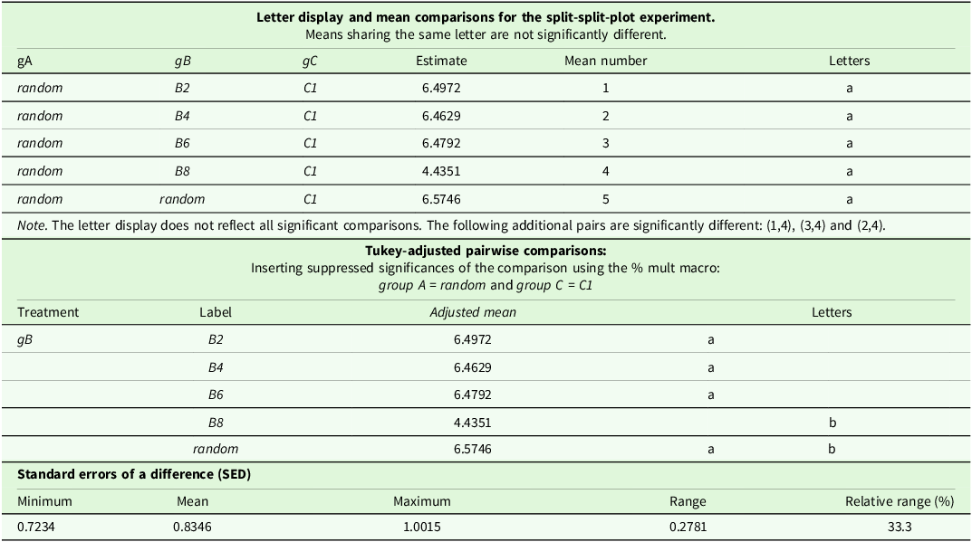
In addition, all the main effects of the three factors (gA, gB and gC) are also significant (P value < 0.05). The percentage total variability accounted for by each random effect is displayed in the last column of the covariance parameter section of Table 7. The largest portion (23.6 %) of the total variation in the wheat yield is attributed to the traditional (random) levels of irrigation treatments (gB.B.sB), and the residual error (14.9 %). Since the three-way interaction is highly significant, we investigate the effect of one factor while holding the other two constant. Supplementary Boxes 12(a) and (b) present the syntax used to generate the mean comparisons for the SSP experiment. Table 8 displays part of the output for the mean comparisons.
Letter display and mean comparisons for the split-split-plot Experiment. Part of output: group B sliced by group A.group C

Note: gB represents group B; B2, B4, B6 and B8 represent the fixed levels of factor B; random represents the set of all random levels associated with factor B; Corresponding notation is used for factors A and C (i.e., gA, and gC).
The letter displays from the grouping of means based on significance was produced by the SLICE option, which sometimes cannot fully display all significant differences, especially when there is heterogeneity in the SED’s. However, the method can deal with this problem if it is implemented in the % mult macro. Hence, it is important to use the macro to get the adjusted pairwise comparisons and these significant differences. The results from the adjusted pairwise comparisons are the same as the results from the grouping means in Table 8. However, letter ‘a’ on mean number 4 was dropped and letter ‘b’ was added on mean numbers 4 and 5 in the grouping of means output in the adjusted pairwise comparison section in order to insert the suppressed significances of the comparison of the affected factor levels. This case did not occur in the previous examples (see Tables 3 and 6) because of the relatively homogeneous SED values. The letter display from the adjusted pairwise comparison shows that the mean of the fixed levels B2, B4 and B6 are not significantly different across the levels of the other two factors (gA.gC) at α = 0.05. In addition, the SED exhibited moderate variability, with a relative range of 33.3 %. (0.2781/0.8346), which is expected and manageable in the context of interpreting pairwise comparisons. This study opts to report SED as the primary measure for mean comparisons because it provides a consistent and interpretable measure of the variability associated with pairwise mean differences.
The random effects for main plots and split-split-plots were removed here because the variances converged to zero. This was mainly done to achieve agreement between the results obtained in SAS and R. A better approach for designed experiments with balanced data such as given here is to allow the variances for these error variances to become negative, thus reproducing classical ANOVA F-tests. This approach is available in SAS using the NOBOUND option. For details see Frey et al. (Reference Frey, Hartung, Ogutu and Piepho2024).
Discussion
The application of the proposed procedures and syntaxes was demonstrated using simulated data. Illustration examples were used to generate the combined analysis of variance in different designs of experiments that involve factors comprising both fixed and random levels. The approach builds on the partitioning method proposed by Chaka and Njuho (Reference Chaka and Njuho2021, Reference Chaka and Njuho2022), extending it to facilitate a broader analysis of variance using the full dataset. SAS PROC GLIMMIX and CRAN software provided useful computational tools for implementing the proposed approach. A significant benefit of the proposed framework is that it integrates inferential assessment of fixed effects with explicit quantification of variability attributable to random effects. Tables 2, 5, and 7 illustrate this dual capability: fixed effects are tested via their P values, whereas the random effects are evaluated through their proportion of total variance. Such joint reporting allows one to determine not only whether significant effects exist, but also which random sources meaningfully drive overall variability. For instance, traditional methods of soil treatment (gA.A.sA) contribute a substantially larger share of variance than lime/sulphur incorporation techniques (gB.B.sB) in barley yield (see Table 2), underscoring differences in practical relevance that extend beyond statistical significance. In addition, a comprehensive assessment of the impact of new farming practices relative to traditional practices was conducted, explicitly accounting for pre-history effects (see Tables 3, 4, 6, and 8), thereby clarifying their influence on the response variable. This dual perspective strengthens interpretation and supports more informed modelling and decision-making in complex experimental settings.
While the proposed approach demonstrates practical utility, the illustrative cases also highlight two important limitations that warrant discussion. First, as one of the illustrative cases, we applied the proposed approach to a repeated-measures design using an AR(1) covariance structure. With only four time points, the estimation of the AR(1) correlation depends on a limited number of adjacent lag correlations, which necessarily limits its precision. Nevertheless, AR(1) remains a reasonable and interpretable choice in this context, as it parsimoniously captures the expected decay of correlation with distance in time while requiring estimation of only a single correlation parameter. Although commonly used in applied longitudinal studies, there are many other serial correlation structures that could be used here (Krone et al., Reference Krone, Albers and Timmerman2017; Muhammad, Reference Muhammad2023). This example highlights that, while the proposed approach can be illustrated effectively, its performance under more complex variance-covariance structures warrants further investigation. Second, the present study did not pursue formal hypothesis testing, focusing instead on estimation and comparative assessment. However, this restriction is largely methodological rather than conceptual. Recent developments indicate that extensions toward formal inference are feasible within the same modelling framework. For instance, the tolerance interval approach proposed by Francq et al. (Reference Francq, Lin and Hoyer2019; Eq. 26) is straightforward to implement using standard mixed-model software for simple variance components models, such as those considered in our first and third examples. Taken together, these limitations suggest several promising directions for future research.
As the current framework accommodates flexible covariance structures, including non-linear specifications, future research should focus on extending the proposed framework toward formal hypothesis testing procedures to settings where such assumptions are relaxed. In particular, recent tolerance interval-based methods provide a promising and practically implementable direction for inference under simple variance components models.
Conclusions
New methods and machinery are continually developed to improve production efficiency, necessitating effective ways to evaluate them against existing techniques. This study extends the partitioning approach by proposing a flexible linear mixed-model framework that integrates both fixed and random effects within a single model. The approach enables comprehensive analysis of variance using full datasets in SAS and CRAN environments, facilitating combined analyses in factorial studies involving factors with both fixed and random levels. It is therefore recommended that researchers adopt full-factorial modelling, with implementations such as the insert-and-absorb algorithm in SAS or equivalent procedures in R, to achieve a more integrated understanding of factor effects and their interactions.
Supplementary material
The supplementary material for this article can be found at https://doi.org/10.1017/S0021859626100653.
Acknowledgments
The authors acknowledge the Trengove Consulting and GRDC projects (DAS 905-011RTX and TGC2304-002RTX) for providing access to Bute on-farm trials data, which was instrumental in conducting part of this research.
Author contributions
Lyson Chaka, Peter Njuho and Hans-Peter Piepho conceived and designed the study. Lyson Chaka and Jean-Claude Malele-Majika conducted data gathering. Lyson Chaka and Hans-Peter Piepho performed statistical analyses. All authors wrote the article.
Funding statement
This research received no specific grant from any funding agency, commercial or not-for-profit sectors.
Competing interests
The authors declare there are no conflicts of interest.
Ethical standards
Not applicable.