1 Introduction
Among the surprising properties of dilute granular flows is the low propagation speed of pressure inhomogeneities. As a consequence, the speed of sound in dilute granular flows is of the order of
 $10~\text{cm}~\text{s}^{-1}$
(Savage Reference Savage1988; Amarouchene & Kellay Reference Amarouchene and Kellay2006; Huang et al.
Reference Huang, Miao, Zhang, Yun and Wei2006; Boudet, Cassagne & Kellay Reference Boudet, Cassagne and Kellay2009), which allows us to easily generate supersonic flows in a simple laboratory setting and to create shock fronts when these flows interact with an obstacle. These shock fronts show similarities with their counterparts in molecular gases (Rericha et al.
Reference Rericha, Bizon, Shattuck and Swinney2001; Boudet & Kellay Reference Boudet and Kellay2010). These granular shock waves can be attached or detached (Hákonardóttir & Hogg Reference Hákonardóttir and Hogg2005) in the same way as for gases (Anderson Reference Anderson1990). Moreover, an obstacle propagating in a granular medium generates a Mach cone in a shallow granular fluid (Heil et al.
Reference Heil, Rericha, Goldman and Swinney2004) and in a dilute flow (Amarouchene & Kellay Reference Amarouchene and Kellay2006). The opening of the Mach cone provides a determination of these low sound speeds. Granular shocks in dense free surface flows have received special attention because they are related to avalanche protection dams (Faug et al.
Reference Faug, Childs, Wyburn and Einav2015). Many configurations were analysed such as oblique shocks, detached or attached bow shocks (Gray & Cui Reference Gray and Cui2007; Johnson & Gray Reference Johnson and Gray2011), crater formation (Boudet, Amarouchene & Kellay Reference Boudet, Amarouchene and Kellay2006) and analogies with hydraulic jumps in shallow-water flows have been found (Gray, Tai & Noelle Reference Gray, Tai and Noelle2003; Boudet, Amarouchene & Kellay Reference Boudet, Amarouchene and Kellay2007; Mejean, Faug & Einav Reference Mejean, Faug and Einav2017).
The second feature of granular media is their dissipative nature. Binary collisions between particles are inelastic and lead to an important energy dissipation (Grossman, Zhou & Ben-Naim Reference Grossman, Zhou and Ben-Naim1997). Dilute granular flows are thus described as dissipative gases (Savage & Jeffrey Reference Savage and Jeffrey1981; Haff Reference Haff1983; Goldhirsch Reference Goldhirsch2003). The theoretical framework for the description of these flows is the granular kinetic theory which is derived from the inelastic Boltzmann equation (Lun et al. Reference Lun, Savage, Jeffrey and Chepurniy1984). The hydrodynamic equations governing granular flows are analogous to the Navier–Stokes equations with specific additional terms due to this inelastic dissipation (Goldshtein & Shapiro Reference Goldshtein and Shapiro1995; Brilliantov & Pöschel Reference Brilliantov and Pöschel2003; Andreotti, Forterre & Pouliquen Reference Andreotti, Forterre and Pouliquen2012). These equations which model flows near the local thermodynamic equilibrium reproduce the behaviour of dilute granular flows despite the fact that velocity distributions in a granular medium are rarely Gaussian. As an illustration, supersonic dilute granular flows around a triangular obstacle were found to be well described by these continuous equations, as shown in Rericha et al. (Reference Rericha, Bizon, Shattuck and Swinney2001). The blast dynamics in a granular gas is also well described by these equations as shown in Barbier, Villamaina & Trizac (Reference Barbier, Villamaina and Trizac2015). Furthermore, the study of granular gases provides prototypical dissipative media on which different theories of the role of dissipation can be tested. Plasmas are another example of a highly dissipative medium where shock fronts and their properties are of great interest. For example in Gregori et al. (Reference Gregori, Ravasio, Murphy, Schaar, Baird, Bell, Benuzzi-Mounaix, Bingham, Constantin and Drake2012), it is shown how the shock front presence during galaxy formation permits us to explain the appearance of magnetic fields in space. A better understanding of shock front structure in granular gases could provide useful information about the role of dissipation for shocks in other media such as a plasma although the nature of the dissipative mechanisms is different.
Supersonic flows around an obstacle are characterized by the existence of a shock front. For strong normal shock waves, this is the region where the supersonic flow becomes subsonic. In this case, it has been shown that the velocity distributions in the front can be very far from Gaussian distributions. They actually show a bimodal structure with two distinct peaks in molecular gases (Holtz & Muntz Reference Holtz and Muntz1983; Pham-Van-Diep, Erwin & Muntz Reference Pham-Van-Diep, Erwin and Muntz1989), in granular gases (Boudet, Amarouchene & Kellay Reference Boudet, Amarouchene and Kellay2008; Vilquin, Boudet & Kellay Reference Vilquin, Boudet and Kellay2016) and in plasmas (Mazouffre et al. Reference Mazouffre, Vankan, Engeln and Schram2001; Vankan et al. Reference Vankan, Mazouffre, Engeln and Schram2005). While hydrodynamics equations remain valid in describing slightly supersonic regimes and weak shock waves, with nearly Gaussian velocity distributions, in molecular gases (Muntz & Harnett Reference Muntz and Harnett1969) and in granular gases (Rericha et al. Reference Rericha, Bizon, Shattuck and Swinney2001), they are not suitable for strong shocks at high Mach numbers. For molecular gases, Mott-Smith (Reference Mott-Smith1951) proposed a description of shock fronts by considering that the velocity distributions are bimodal. Using a bimodal velocity distribution to solve the Boltzmann equation leads to a better description of the shock front than that obtained by the resolution of the hydrodynamic equations. A similar description in a dissipative granular medium has not been attempted yet.
In this work, we propose to apply this bimodal description to dissipative granular gases. A granular gas is a dilute flow where particles interact with binary collisions, very different from dense granular flows where few particles can have prolonged contact. We study the problem of a rectangular obstacle moving in a vibrated granular medium. In a restricted area centred on the symmetry axis of the flow, this problem could be considered similar to a one-dimensional piston problem. This problem has already been analysed for gases by Landau & Lifchitz (Reference Landau and Lifchitz1967). The obstacle moving at a constant speed
 $V_{obs}$
, generates, after a transient, a one-dimensional shock front of high intensity moving at a constant speed
 $V_{front}$
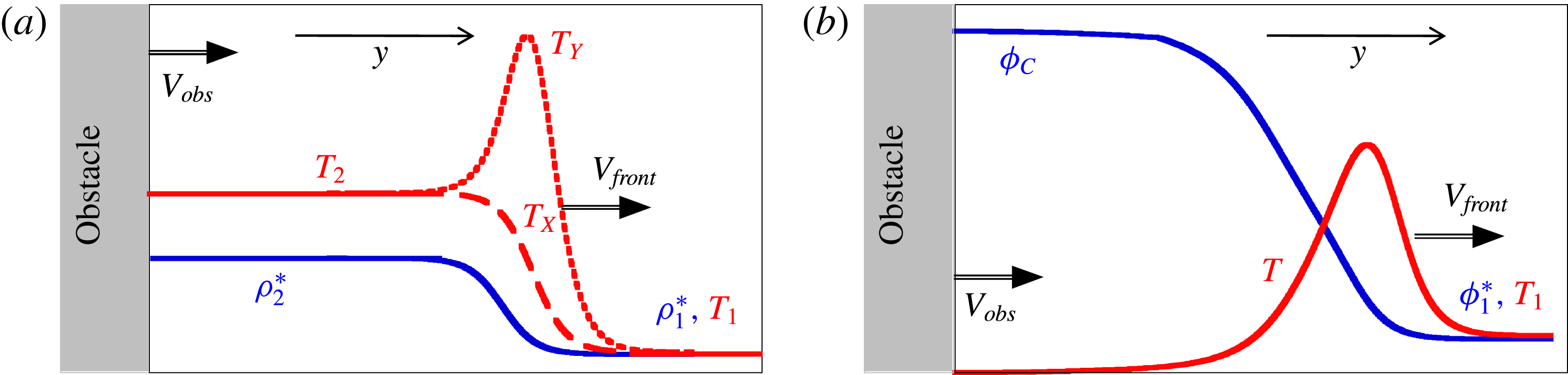
. Density and temperature profiles generated by the obstacle displacement are plotted in figure 1(a) for a molecular gas. Far from the obstacle, the initial gas has a temperature
 $T_{1}$
, a density
 $\unicode[STIX]{x1D70C}_{1}^{\ast }$
and a zero mean velocity. Near the obstacle, the gas is compressed to a denser value
 $\unicode[STIX]{x1D70C}_{2}^{\ast }$
, heated to a higher temperature
 $T_{2}$
and propagates at the obstacle speed. In the reference frame of the shock front, the supersonic flow is the initial gas and the subsonic flow is the denser gas close to the obstacle. These two gases are at thermodynamic equilibrium. The shock front is the non-equilibrium region, connecting these two flows, and where strong variations in physical quantities occur. Its thickness is of the same order of magnitude as the mean free path
 $\unicode[STIX]{x1D706}$
evaluated in the initial gas. In this region, the velocity distributions show a two-peak structure because supersonic and subsonic gases coexist. Macroscopic variables on either side of the front are connected by Rankine–Hugoniot equations, which allow us to determine
 $\unicode[STIX]{x1D70C}_{2}^{\ast }$
,
 $T_{2}$
and
 $V_{front}$
as functions of
 $\unicode[STIX]{x1D70C}_{1}^{\ast }$
,
 $T_{1}$
and
 $V_{obs}$
. The Mach number of this flow is given by
 $Ma=V_{front}/C_{1}$
, where
 $C_{1}$
is the sound speed in the initial gas. The bimodal structure of the velocity distributions leads to an anisotropy of the temperature (Harnett & Muntz Reference Harnett and Muntz1972; Holian et al.
Reference Holian, Patterson, Mareschal and Salomons1993; Hoover & Hoover Reference Hoover and Hoover2010): for an obstacle propagating along the
 $y$
-axis, the longitudinal temperature (denoted
 $T_{Y}$
) is greater than the transverse temperature (denoted
 $T_{X}$
), as illustrated in figure 1(a). Note that the extent of the shock front is the region where the two temperatures differ.
Schematic of density and temperature profiles generated by a moving obstacle in the
 $y$
-direction in a one-dimensional medium. (a) Molecular gas:
 $T_{Y}$
and
 $T_{X}$
are the longitudinal and transverse temperatures. The gas density
 $\unicode[STIX]{x1D70C}$
is the blue curve.
 $(\unicode[STIX]{x1D70C}_{1}^{\ast },T_{1})$
and
 $(\unicode[STIX]{x1D70C}_{2}^{\ast },T_{2})$
are respectively the density and temperature values of supersonic and subsonic gases on either side of the shock front linked by Rankine–Hugoniot conditions (see § 2). (b) Granular gas:
 $T$
is the temperature. The gas volume fraction
 $\unicode[STIX]{x1D719}$
is the blue curve.
 $(\unicode[STIX]{x1D719}_{1}^{\ast },T_{1})$
are the initial value of volume fraction and temperature.
 $\unicode[STIX]{x1D719}_{C}$
is the random close-packing volume fraction.

The piston problem has also been considered in a granular medium in recent numerical work by Sirmas & Radulescu (Reference Sirmas and Radulescu2015). They show that an obstacle, propagating in an inelastic gas, also generates a shock front that travels at constant speed. However, the volume fraction and longitudinal temperature profiles illustrated in figure 1(b) show large differences with respect to molecular gases. The temperature reaches a maximum before decreasing near the obstacle to very low values. The volume fraction increases continuously up to its maximum value (
 $\unicode[STIX]{x1D719}_{C}$
, random close-packing volume fraction). For a granular material of spherical particles with a diameter
 $d$
, the volume fraction is
 $\unicode[STIX]{x1D719}=NV_{p}/V$
where
 $N$
is the particle number,
 $V_{p}=\unicode[STIX]{x03C0}d^{3}/6$
and
 $V$
the volume of the region of interest. Goldshtein, Shapiro & Gutfinger (Reference Goldshtein, Shapiro and Gutfinger1996) had previously analysed this device in the context of granular hydrodynamic equations and showed a qualitative agreement with the simulations. In particular the authors explain the shape of the profiles by the leading role of inelastic dissipation. In the shock front, the inelastic gas is compressed and the temperature and the volume fraction increase. As the number of inelastic collisions increases, the energy decreases as we progress in the shock front. The gas temperature decreases continuously to zero while the volume fraction increases to a maximum value
 $\unicode[STIX]{x1D719}_{C}$
.
Sirmas & Radulescu (Reference Sirmas and Radulescu2015) do not focus on the shock front in their simulations. They do not measure temperature and velocity distributions along each axis. Goldshtein et al. (Reference Goldshtein, Shapiro and Gutfinger1996) use hydrodynamic equations, which are not suitable to describe the shock front for strong shock waves with bimodal velocity distributions. One of the objectives of the present work is a careful description of normal shocks in granular gases; particularly focusing on the velocity distributions and temperature along each axis.
Note the following specificity of the granular piston: without power injection, a granular gas will collapse and its temperature will decrease to zero because of inelastic collisions. Goldshtein et al. (Reference Goldshtein, Shapiro and Gutfinger1996) bypass this difficulty by taking a zero temperature for the initial supersonic gas, so the Mach number is infinite. Sirmas & Radulescu (Reference Sirmas and Radulescu2015) use inelasticity depending on a velocity threshold. Shocks are elastic if they occur between two particles whose velocity difference is below a defined threshold. They become inelastic if the velocity difference is above this threshold. This procedure permits us to maintain the gas temperature to a value depending on this threshold. However, to probe the inelastic behaviour of this inelastic gas in the disturbed area, it is necessary to use a sufficiently high obstacle velocity. In other words, the front propagation speed is limited to large Mach numbers; this procedure does not allow us to approach the subsonic–supersonic transition.
We here use a rectangular obstacle displaced a vibrated box containing a granular medium. The energy injected by the walls of the container compensates dissipation due to inelastic collisions and permits us to obtain a vibrated granular gas with a well-defined granular temperature (Ogawa Reference Ogawa1978). By controlling this temperature value and obstacle velocity, this set-up allows us to access to a wide range of Mach numbers and observe the subsonic–supersonic transition in dilute granular flows.
Sections 2 and 3 of this paper present the Mott-Smith model for gases and its adaptation for a granular medium, which we term the bimodal inelastic model. Section 4 presents the experimental set-up of the granular piston in a vibrated box. Section 5 shows all the results obtained at different Mach numbers and their analysis based on the inelastic bimodal model. The paper then ends with a discussion on the role of dissipation in the shock front in § 6, and a final short conclusion.
2 The Rankine–Hugoniot relations and the Mott-Smith model
The work undertaken in this section consists of presenting the theory of one-dimensional shock waves for dilute gases proposed in 1951 by Mott-Smith before extending it to an inelastic gas such as a granular gas in § 3. Let us first introduce the jump relations established by Rankine (Reference Rankine1870) and Hugoniot (Reference Hugoniot1887). These relations permit us to link macroscopic properties of supersonic and subsonic gases on either side of the shock front. They are obtained by writing the conservation laws of energy, momentum and mass for a non-dissipative gas and can be written for a perfect gas with
 $n$
degrees of freedom in the reference frame of the shock front as:
 $$\begin{eqnarray}\displaystyle \left.\begin{array}{@{}c@{}}\displaystyle \frac{\unicode[STIX]{x1D70C}_{2}^{\ast }}{\unicode[STIX]{x1D70C}_{1}^{\ast }}=\frac{n+1}{1+nMa^{-2}},\\ \displaystyle \frac{V_{2}}{V_{1}}=\frac{1+nMa^{-2}}{n+1},\\ \displaystyle \frac{T_{2}}{T_{1}}=\frac{(1+nMa^{-2})((n+2)Ma^{2}-1)}{(n+1)^{2}}.\end{array}\right\} & & \displaystyle\end{eqnarray}$$
The values of the mean velocity
 $V_{2}$
, the temperature
 $T_{2}$
and the number density
 $\unicode[STIX]{x1D70C}_{2}^{\ast }$
(far from the front) describing the subsonic flow can be calculated from their counterparts describing the supersonic flow (
 $V_{1}$
,
 $T_{1},\unicode[STIX]{x1D70C}_{1}^{\ast }$
) for different Mach numbers
 $Ma=V_{1}/C_{1}$
. However, these values give no indication of the density profile which requires an adequate description of the front.
Mott-Smith (Reference Mott-Smith1951) makes a very simple hypothesis. Because of the presence of supersonic and subsonic gases in the shock front, the velocity distribution in this region is bimodal and is the sum of two Gaussian distributions. The proportions of each peak varies across the shock front. For a shock wave propagating along the axis
 $y$
, the velocity distribution function is written
 $f=f_{1}+f_{2}$
with:
 $$\begin{eqnarray}f_{i}(\boldsymbol{c})=\frac{\unicode[STIX]{x1D70C}_{i}(y)}{(2\unicode[STIX]{x03C0}k_{B}T_{i}/m)^{3/2}}\exp \left(-\frac{(\boldsymbol{c}-V_{i}\boldsymbol{e}_{\boldsymbol{y}})^{2}}{2k_{B}T_{i}/m}\right),\quad i=1,2.\end{eqnarray}$$
Here
 $\boldsymbol{c}=u\boldsymbol{e}_{\boldsymbol{x}}+v\boldsymbol{e}_{\boldsymbol{y}}+w\boldsymbol{e}_{\boldsymbol{z}}$
is the velocity vector of a particle;
 $k_{B}$
and
 $m$
are respectively the Boltzmann constant and the mass of the particle. The number densities
 $\unicode[STIX]{x1D70C}_{i}(y)$
represent respectively the local density of supersonic particles (
 $i=1$
) and subsonic particles (
 $i=2$
). These equations are usually written in the reference frame of the shock front. By using this distribution in the Boltzmann equation, conservation laws permit us to obtain Euler equations with two populations. These equations lead to mean velocities, temperatures and density values of the two gases which obey the Rankine–Hugoniot conditions (2.1). To find the density profile in the shock front, Mott-Smith then calculates the moment of order 2 of the longitudinal speed with the Boltzmann equation and obtains the following closure relation:
 $$\begin{eqnarray}\frac{\unicode[STIX]{x2202}\unicode[STIX]{x1D70C}_{1}(y)}{\unicode[STIX]{x2202}y}=-B\frac{\unicode[STIX]{x1D70C}_{1}(1-\unicode[STIX]{x1D70C}_{1}/\unicode[STIX]{x1D70C}_{1}^{\ast })}{\unicode[STIX]{x1D706}},\end{eqnarray}$$
where
 $\unicode[STIX]{x1D706}$
is the mean free path in the supersonic gas. The coefficient
 $B$
only depends on the Mach number and
 $n$
. This equation is used to find the density profile of each population:
 $$\begin{eqnarray}\displaystyle \unicode[STIX]{x1D70C}_{1}(y)=\frac{\unicode[STIX]{x1D70C}_{1}^{\ast }}{1+\exp (-By/\unicode[STIX]{x1D706})},\quad \unicode[STIX]{x1D70C}_{2}(y)=\frac{\unicode[STIX]{x1D70C}_{2}^{\ast }}{1+\exp (By/\unicode[STIX]{x1D706})}. & & \displaystyle\end{eqnarray}$$
The shock front width is given by
 $L_{MS}=4\unicode[STIX]{x1D706}/B$
. Note that the bimodal distribution proposed by Mott-Smith is not a solution of the Boltzmann equation to describe the shock front. Indeed the calculation with a moment of order 3 leads to a similar closure equation but with a coefficient
 $B$
which is slightly different. However, the model works reasonably well when compared to observations. For a gas of hard spheres, the width variation with the Mach number complies with numerical simulations with better than 10 % accuracy (Lumpkin & Chapman Reference Lumpkin and Chapman1992). Actually, the results given by Mott-Smith quite faithfully reflect macroscopic variables and their evolution through the shock front.
Despite the fact that the Mott-Smith model is a good approach to describe the shock, it does not accurately reflect the shape of the velocity distributions in the shock front, along the longitudinal axis, for large Mach number values. The velocity distributions, experimentally measured by Pham-Van-Diep et al. (Reference Pham-Van-Diep, Erwin and Muntz1989) in helium for
 $Ma=25$
, show that there is an overpopulation at intermediate speeds. It has been shown that in a granular shock fronts, this overpopulation is mainly due to particles produced by collisions between the subsonic and the supersonic particles (Vilquin et al.
Reference Vilquin, Boudet and Kellay2016). These results show that a three-population model could be more relevant for shock waves generated with large Mach number values. For a first application to a dissipative medium, we limit our study to a two-population model.
According to the Mott-Smith model, the total temperatures calculated along each axis are different in the shock front. For a shock wave propagating along
 $y$
-axis,
 $T_{Y}$
is always larger than
 $T_{X}$
(as shown in figure 1
a) and the difference is given by:
 $$\begin{eqnarray}T_{Y}-T_{X}=\frac{\unicode[STIX]{x1D70C}_{1}(y)\cdot \unicode[STIX]{x1D70C}_{2}(y)}{(\unicode[STIX]{x1D70C}_{2}(y)+\unicode[STIX]{x1D70C}_{1}(y))^{2}}\frac{m(V_{1}-V_{2})^{2}}{k_{B}}.\end{eqnarray}$$
This equation gives the temperature difference profile as a function of the position along the direction of the flow. The temperature difference is zero on each side of the front, goes through a maximum which occurs when
 $\unicode[STIX]{x1D70C}_{1}(y)=\unicode[STIX]{x1D70C}_{2}(y)$
and is given by:
 $$\begin{eqnarray}(T_{Y}-T_{X})_{MAX}=\frac{m(V_{1}-V_{2})^{2}}{4k_{B}}.\end{eqnarray}$$
This maximum depends only on the Mach number via the velocity jump relation (2.1). If the speed of the shock front approaches the speed of sound, the jump becomes increasingly weak and the width of the shock front increases sharply. This is the transition to a subsonic flow: changes in macroscopic quantities such as the characteristic lengths go from the mean free path for supersonic flows to macroscopic scales for subsonic flows and these changes are well described by the Mott-Smith model. Note that
 $Ma=1$
is the Mach number for which
 $T_{Y}(y)=T_{X}(y)$
and
 $L_{MS}\rightarrow \infty$
: the shock front disappears.
3 The inelastic bimodal model
3.1 Granular kinetic theory
From the Boltzmann equation for inelastic gases, Lun derived the hydrodynamic equations (Lun et al.
Reference Lun, Savage, Jeffrey and Chepurniy1984): These are written for a one-dimensional flow along the
 $y$
-axis as:
 $$\begin{eqnarray}\displaystyle & \displaystyle \frac{\unicode[STIX]{x2202}}{\unicode[STIX]{x2202}y}[\unicode[STIX]{x1D719}V]=0, & \displaystyle\end{eqnarray}$$
 $$\begin{eqnarray}\displaystyle & \displaystyle \frac{\unicode[STIX]{x2202}}{\unicode[STIX]{x2202}y}[\unicode[STIX]{x1D719}V^{2}+P]=0, & \displaystyle\end{eqnarray}$$
 $$\begin{eqnarray}\displaystyle & \displaystyle \frac{\unicode[STIX]{x2202}}{\unicode[STIX]{x2202}y}\left[\unicode[STIX]{x1D719}V\left(\frac{1}{2}V^{2}+\frac{n}{2}T+P\right)\right]=\unicode[STIX]{x1D6E4}_{G}, & \displaystyle\end{eqnarray}$$
where
 $V=\langle v\rangle$
is the longitudinal mean velocity along the
 $y$
-axis. The transverse mean velocity
 $\langle u\rangle =0$
in our one-dimensional model.
 $T$
is the granular temperature and is defined by
 $T=\unicode[STIX]{x1D6FF}\boldsymbol{c}^{2}/3$
(
 $\unicode[STIX]{x1D6FF}\boldsymbol{c}$
is the standard deviation of the particle velocity
 $\boldsymbol{c}$
,
 $T_{X}=\unicode[STIX]{x1D6FF}\boldsymbol{u}^{2}$
and
 $T_{Y}=\unicode[STIX]{x1D6FF}\boldsymbol{v}^{2}$
are the temperatures along
 $x$
and
 $y$
) and
 $\unicode[STIX]{x1D719}$
is the volume fraction. We here use the following equation of state to describe a granular gas (Bougie et al.
Reference Bougie, Moon, Swift and Swinney2002) with the pressure
 $P$
given by:
 $$\begin{eqnarray}\displaystyle P=\unicode[STIX]{x1D719}T\unicode[STIX]{x1D712}(\unicode[STIX]{x1D719}),\quad \unicode[STIX]{x1D712}(\unicode[STIX]{x1D719})=1+\frac{2(1+r)\unicode[STIX]{x1D719}}{\left(1-\left(\displaystyle \frac{\unicode[STIX]{x1D719}}{\unicode[STIX]{x1D719}_{C}}\right)^{(4/3)\unicode[STIX]{x1D719}_{C}}\right)}, & & \displaystyle\end{eqnarray}$$
where
 $r$
is the coefficient of inelasticity, and
 $\unicode[STIX]{x1D719}_{C}=0.65$
is the random close-packing volume fraction. The main difference with molecular gases is the term
 $\unicode[STIX]{x1D6E4}_{G}$
, which is the energy dissipation due to inelastic collisions between particles and can be written in (Bougie et al.
Reference Bougie, Moon, Swift and Swinney2002):
 $$\begin{eqnarray}\unicode[STIX]{x1D6E4}_{G}=-\frac{12(1-r^{2})}{d\sqrt{\unicode[STIX]{x03C0}}}\unicode[STIX]{x1D719}^{2}T^{3/2}.\end{eqnarray}$$
Note that the Rankine–Hugoniot relations are invalid for granular shock waves because of the energy dissipation term. From the granular kinetic theory the speed of sound with
 $6$
freedom degrees is given (Savage Reference Savage1988) by:
 $$\begin{eqnarray}C_{1}=\sqrt{\unicode[STIX]{x1D712}T\left(1+\frac{1}{3}\unicode[STIX]{x1D712}+\frac{\unicode[STIX]{x1D719}}{\unicode[STIX]{x1D712}}\frac{\unicode[STIX]{x2202}\unicode[STIX]{x1D712}}{\unicode[STIX]{x2202}\unicode[STIX]{x1D719}}\right)}.\end{eqnarray}$$
In the following, unless otherwise specified, we will use the term ‘Mach number’
 $Ma$
for the free stream Mach number where the speed of sound
 $C_{1}$
is calculated in the vibrated granular gas
 $(\unicode[STIX]{x1D719}=\unicode[STIX]{x1D719}_{1}^{\ast },V=V_{1},T=T_{1})$
far from the shock front.
3.2 The bimodal assumption
Now for the shock front, we make the same assumption as Mott-Smith: the velocity distributions are bimodal and can be written as:
 $f=f_{1}+f_{2}$
where
 $f_{i}$
is given by:
 $$\begin{eqnarray}f_{i}(\boldsymbol{c})=\frac{\unicode[STIX]{x1D719}_{i}(y)}{(2\unicode[STIX]{x03C0}T_{i})^{3/2}}\exp \left(-\frac{(\boldsymbol{c}-V_{i}\boldsymbol{e}_{\boldsymbol{y}})^{2}}{2T_{i}}\right),\quad i=1,2.\end{eqnarray}$$
The hydrodynamic equations for a model of two populations are then written:
 $$\begin{eqnarray}\displaystyle & \displaystyle \frac{\unicode[STIX]{x2202}}{\unicode[STIX]{x2202}y}[\unicode[STIX]{x1D719}_{1}V_{1}+\unicode[STIX]{x1D719}_{2}V_{2}]=\frac{\unicode[STIX]{x2202}M}{\unicode[STIX]{x2202}y}=0, & \displaystyle\end{eqnarray}$$
 $$\begin{eqnarray}\displaystyle & \displaystyle \frac{\unicode[STIX]{x2202}}{\unicode[STIX]{x2202}y}[\unicode[STIX]{x1D719}_{1}V_{1}^{2}+P_{1}+\unicode[STIX]{x1D719}_{2}V_{2}^{2}+P_{2}]=\frac{\unicode[STIX]{x2202}P}{\unicode[STIX]{x2202}y}=0, & \displaystyle\end{eqnarray}$$
 $$\begin{eqnarray}\displaystyle & \displaystyle \frac{\unicode[STIX]{x2202}}{\unicode[STIX]{x2202}y}\left[\unicode[STIX]{x1D719}_{1}V_{1}\left(\frac{n}{2}T_{1}+\frac{1}{2}V_{1}^{2}+P_{1}\right)+\unicode[STIX]{x1D719}_{2}V_{2}\left(\frac{n}{2}T_{2}+\frac{1}{2}V_{2}^{2}+P_{2}\right)\right]=\frac{\unicode[STIX]{x2202}E}{\unicode[STIX]{x2202}y}=\unicode[STIX]{x1D6E4}, & \displaystyle\end{eqnarray}$$
where
 $M$
,
 $P$
and
 $E$
are respectively mass, momentum and energy flows. The energy dissipation
 $\unicode[STIX]{x1D6E4}$
must be derived from the inelastic Boltzmann equation and has not yet been established for strong shock waves in a vibrated granular gas. In these equations, the mean velocity
 $V_{1}$
and temperature
 $T_{1}$
are the known properties of the initial supersonic gas. In our system, we assume that
 $V_{1}$
and
 $T_{1}$
do not vary across the shock front contrary to the volume fraction
 $\unicode[STIX]{x1D719}_{1}$
since the supersonic gas becomes subsonic. This assumption will be justified by the description of energy injection and dissipation in § 3.3. We need to obtain this volume fraction
 $\unicode[STIX]{x1D719}_{1}$
and the properties of the subsonic gas
 $(\unicode[STIX]{x1D719}_{2},V_{2},T_{2})$
. Note that we neglect friction phenomena due to the top and bottom vibrated walls. An additional relation, similar to the closure equation (2.3), is required to solve the system as in the Mott-Smith model in molecular gases. In a previous work, Boudet et al. (Reference Boudet, Amarouchene and Kellay2008) showed the bimodal nature of the velocity distributions in a shock front and a closure relation similar to the one stated above has been found in dilute granular media. We use the following functional form (identical to that proposed by Mott-Smith):
 $$\begin{eqnarray}\unicode[STIX]{x1D719}_{1}(y)=\frac{\unicode[STIX]{x1D719}_{1}^{\ast }}{1+\exp (-y/L)}.\end{eqnarray}$$
It correctly describes the density profile of supersonic particles where
 $4L$
is the counterpart of the shock front width in the Mott-Smith model in molecular gases.
3.3 Energy injection and dissipation
Solving this system requires us to find the expression for the dissipation term. This calculation, for strong shock waves in a vibrated granular gas, presents several difficulties. The velocity distributions in the shock front have complex shapes far from Gaussian distributions. Moreover, in addition to dissipation terms due to inelastic collisions, we have to take into account the energy injection due to the collisions with the vibrated walls. This injection part ensures the existence of the initial vibrated granular gas with a non-zero temperature far from the shock front.
First we consider the dissipation terms due to inelastic collisions. Making the hypothesis of bimodality allows us to decompose the term into three contributions emanating from collisions between two supersonic particles, collisions between two subsonic particles and collisions between a supersonic particle and a subsonic particle which would contribute respectively to the following terms:
 $\unicode[STIX]{x1D6E4}_{1,1}+\unicode[STIX]{x1D6E4}_{2,2}+\unicode[STIX]{x1D6E4}_{1,2}$
. For terms
 $\unicode[STIX]{x1D6E4}_{i,i}$
, for the same kind of particles, we write the granular dissipation in the form (
 $i=1,2$
):
 $$\begin{eqnarray}\unicode[STIX]{x1D6E4}_{i,i}=-\frac{12}{d\sqrt{\unicode[STIX]{x03C0}}}(1-r^{2})\unicode[STIX]{x1D719}_{i}^{2}T_{i}^{3/2},\end{eqnarray}$$
where
 $d$
is the particle diameter. For the term
 $\unicode[STIX]{x1D6E4}_{1,2}$
, we write by adapting a term obtained in Barrat & Trizac (Reference Barrat and Trizac2002) for two-population dissipation:
 $$\begin{eqnarray}\unicode[STIX]{x1D6E4}_{1,2}=-\frac{12}{d\sqrt{\unicode[STIX]{x03C0}}}(1-r^{2})\unicode[STIX]{x1D719}_{1}\unicode[STIX]{x1D719}_{2}\left(T_{1}+\frac{1}{n}(V_{1}-V_{2})^{2}+T_{2}\right)^{3/2}.\end{eqnarray}$$
Along with these considerations, we also need to consider the injection part due to collisions between particles and the top and bottom walls. In the same way as the dissipation part, we use the bimodal assumption to introduce two additional terms,
 $\unicode[STIX]{x1D6E4}_{W1}$
and
 $\unicode[STIX]{x1D6E4}_{W2}$
, in the right-hand side of equation (3.10). These terms are respectively interaction term between walls and supersonic particles, and between walls and subsonic particles. Then the total dissipation term is:
 $$\begin{eqnarray}\unicode[STIX]{x1D6E4}=\unicode[STIX]{x1D6E4}_{1,1}+\unicode[STIX]{x1D6E4}_{2,2}+\unicode[STIX]{x1D6E4}_{1,2}+\unicode[STIX]{x1D6E4}_{W1}+\unicode[STIX]{x1D6E4}_{W2}.\end{eqnarray}$$
In the undisturbed region far from the shock, to obtain an initial granular gas with a non-zero temperature in a stationary state, the dissipation due to inelastic collisions is compensated by the energy injection then
 $\unicode[STIX]{x1D6E4}_{1,1}+\unicode[STIX]{x1D6E4}_{W1}=0$
. The walls inject energy into the system which compensates for the dissipative terms for supersonic particles without obstacle propagation. We assume that this equality remains valid throughout the shock front. In other words, we consider the supersonic particles keep their initial stationary state before they become subsonic. It allows us to assume that
 $V_{1}$
and
 $T_{1}$
are constant. The right-hand side of the dissipation term is reduced to
 $\unicode[STIX]{x1D6E4}=\unicode[STIX]{x1D6E4}_{2,2}+\unicode[STIX]{x1D6E4}_{1,2}+\unicode[STIX]{x1D6E4}_{W2}$
. Note that
 $\unicode[STIX]{x1D6E4}_{W2}$
is unknown. We tested different functional forms for
 $\unicode[STIX]{x1D6E4}$
. As we see below, an adequate form for the dissipation turns out to be:
 $$\begin{eqnarray}\unicode[STIX]{x1D6E4}=-k\frac{12}{d\sqrt{\unicode[STIX]{x03C0}}}(1-r^{2})\unicode[STIX]{x1D719}_{2}^{2}T_{2}^{3/2}.\end{eqnarray}$$
The functional form is similar to that of
 $\unicode[STIX]{x1D6E4}_{2,2}$
, indicating that the major contribution is due to
 $\unicode[STIX]{x1D6E4}_{2,2}$
but
 $k$
is an unknown constant. Note that we have neglected the contribution of
 $\unicode[STIX]{x1D6E4}_{1,2}$
, and we discuss this assumption in § 6.1.
An important question is how the shock width
 $L$
and the dissipation parameter
 $k$
are determined. The two parameters are determined by using a numerical resolution with Euler method (see appendix A) and discussed in § 6, to obtain the best agreement with our experimental measurements. The value of
 $L$
is mainly imposed by the width of the temperature difference
 $T_{Y}-T_{X}$
(shown in figure 10), which has a low sensitivity to
 $k$
values. The other macroscopic quantities (volume fraction
 $\unicode[STIX]{x1D719}$
, mean velocity
 $V$
) permit us to obtain the
 $k$
value. We will show in § 5 that normal shock fronts in dilute granular media can be described in a satisfactory manner.
4 Measurement methods and experimental set-up
4.1 Properties of the vibrated granular gas without obstacle displacement
A thin horizontal box (with internal dimensions
 $36\times 21\times 0.3$
cm) contains a granular medium of steel balls (diameter
 $d=1$
mm). Here, a homogeneous granular gas is obtained when the box is vibrated vertically using an electromagnetic shaker with frequencies ranging from
 $28$
to
 $46$
Hz and an acceleration between
 $1.5$
and
 $4$
 $g$
where gravity
 $g=9.81~\text{m}~\text{s}^{-2}$
. With a vibration amplitude
 $A=1$
mm, the system enables to obtain an homogeneous granular gas with a volume fraction
 $\unicode[STIX]{x1D719}_{1}^{\ast }$
varying between
 $0.07$
and
 $0.14$
. The cell consists of a lower anodized aluminium plate, an upper glass plate and aluminium spacers of 3 mm thickness.
To obtain the local volume fraction
 $\unicode[STIX]{x1D719}$
and particle velocities
 $\boldsymbol{c}$
in the box plane (
 $x$
and
 $y$
axis), the reflected light from the beads is collected with a fast camera working at
 $4000$
frames per second, allowing an accurate particle tracking. Each steel bead is a spherical mirror reflecting light from a spot with a radius smaller than the bead diameter. Particle positions and velocities are obtained from the images with the software ImageJ (see photographs in figures 4, 5, 7 and 11). Calculations of velocity distributions and macroscopic values are realized with a home-made program on the software Matlab. Details on experimental set-up and calculations are given in Vilquin (Reference Vilquin2015), Vilquin et al. (Reference Vilquin, Boudet and Kellay2016).
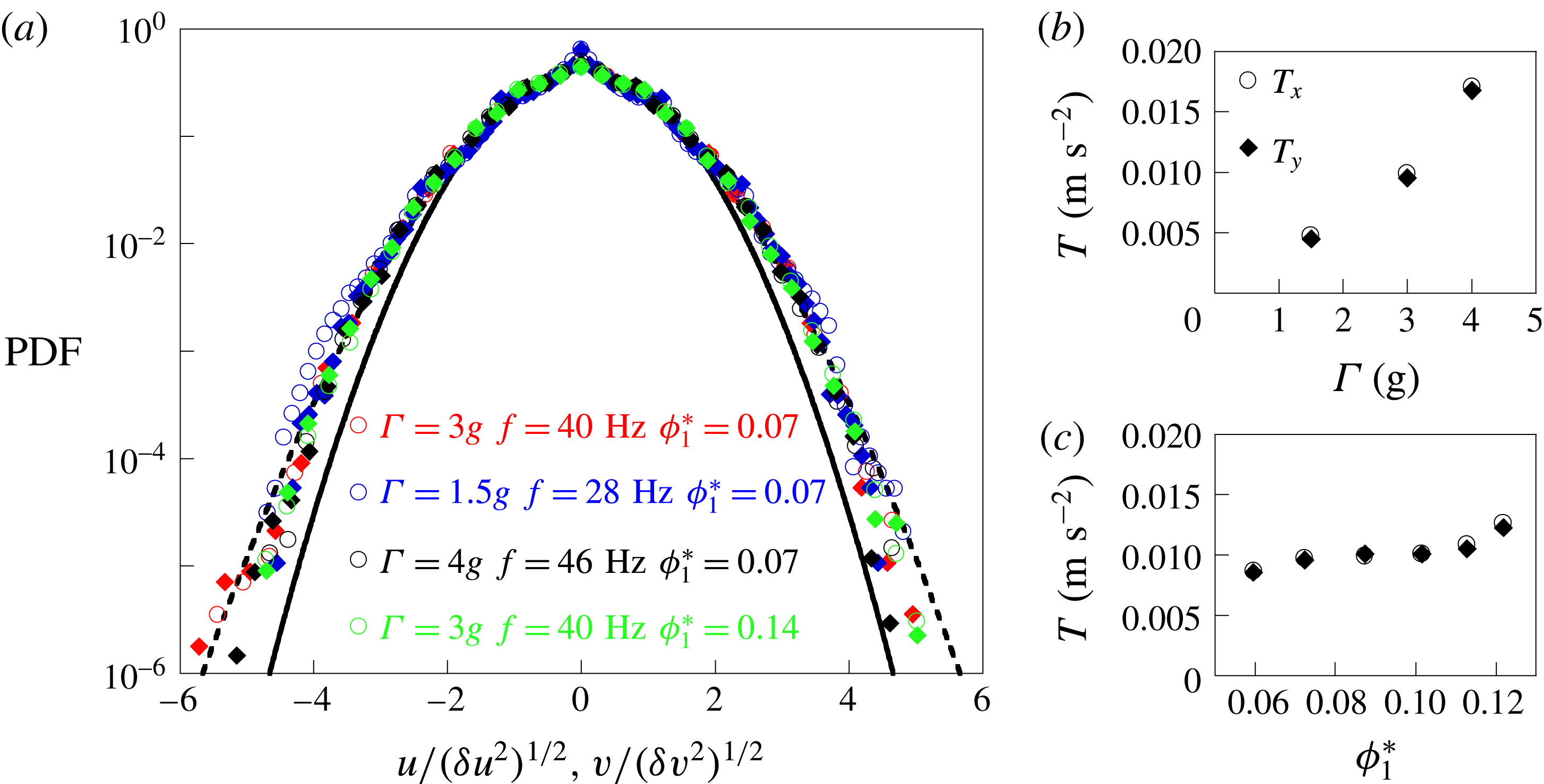
Considering the vibration conditions described above, the granular gas is homogeneous in the whole box in agreement with experiments carried out by Roeller et al. (Reference Roeller, Clewett, Bowley, Herminghaus and Swift2011). The velocity distributions (probability distribution function: PDF) depicted in figure 2(a) are not strictly a Gaussian, as already observed in previous studies (Rouyer & Menon Reference Rouyer and Menon2000; Van Zon & Mackintosh Reference Van Zon and Mackintosh2004), especially for flat walls (Windows-Yule & Parker Reference Windows-Yule and Parker2013). Note that the PDF shape does not change in the range of parameters used in our experiments. The gas temperature
 $T_{1}$
, extracted from particle velocities, is plotted in figure 2(b,c). This temperature increases with the reduced acceleration but is roughly constant versus the gas volume fraction. Energy transfers between a vibrated wall and a granular system are not well described (Windows-Yule et al.
Reference Windows-Yule, Rosato, Parker and Thornton2015). For the initial vibrated granular gas in these experiments, it is observed that the reduced acceleration of the walls plays a leading role in the control of the gas temperature (Aumaître et al.
Reference Aumaître, Fauve, McNamara and Poggi2001). This temperature is used to calculate the sound speed
 $C_{1}$
(see (3.6)) by taking
 $r=0.95$
for steel beads. Our measurements are realized for different parameters:
 $\unicode[STIX]{x1D719}_{1}^{\ast }=0.07$
with
 $C_{1}=0.1,$
 $0.15$
and
 $0.2~\text{m}~\text{s}^{-1}$
and
 $\unicode[STIX]{x1D719}_{1}^{\ast }=0.14$
with
 $C_{1}=0.17~\text{m}~\text{s}^{-1}$
. The speed of sound in the granular gas can thus be directly controlled by the shaker acceleration and to a small extent by the volume fraction of particles.
(a) Velocity distributions normalized by the standard deviation along both axes (circles
 $PDF(v)$
along
 $y$
axis, plain diamonds
 $PDF(u)$
along
 $x$
axis). The black curves are fits using the functional shape
 $\exp (-[c_{i}^{2}/b_{i}]^{a})$
with
 $a=1$
for the solid line and
 $a=0.75$
for the dashed line. (b) Temperatures along each axis as a function of the reduced acceleration for
 $\unicode[STIX]{x1D719}_{1}^{\ast }=0.07$
. (c) Temperatures as function of vibrated granular gas density for
 $\unicode[STIX]{x1D6E4}=3g$
and
 $f=40~\text{Hz}$
.

4.2 The granular shock front
To generate shock waves in the vibrated granular gas, a rectangular obstacle, with 7 cm width and 3 mm thickness, is translated at a constant speed
 $V_{obs}$
(along the
 $y$
-axis from left to right) varying between
 $0.07$
and
 $2~\text{m}~\text{s}^{-1}$
in the granular gas. It corresponds to a range of Mach numbers varying between
 $0.5$
and
 $13$
. After a transient, it produces upstream a volume fraction bump which propagates in the vibrated granular medium at constant speed denoted
 $V_{front}$
. For supersonic obstacle displacements, the shock front reaches a stationary state (see details in Vilquin Reference Vilquin2015 and Vilquin et al.
Reference Vilquin, Boudet and Kellay2016). It allows us to study the problem in the reference frame of the front. Then the initial vibrated granular gas, far from the front, becomes the supersonic gas with a mean longitudinal velocity
 $V_{1}=V_{front}$
and temperature
 $T_{1}$
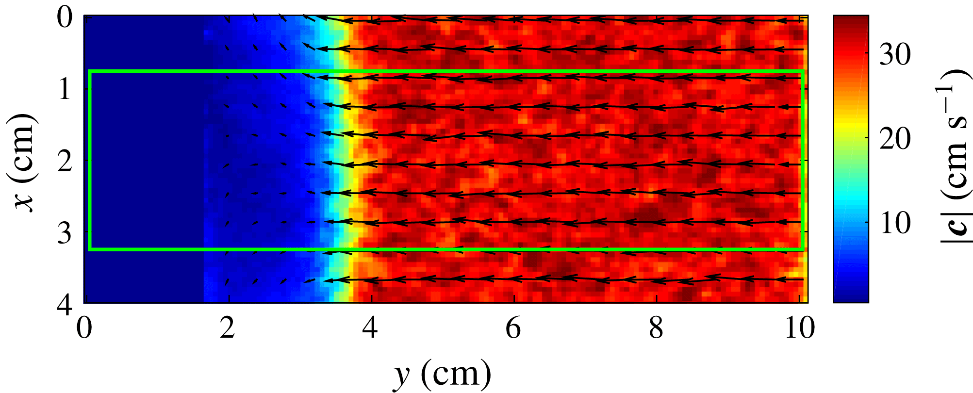
, determined by vibration conditions. In this way, we calculated a temporal average of the velocity fields in the reference frame of the shock front shown in figure 3. For the measurements shown in § 5, we restrict the region of interest to a width of 25 mm, centred on the symmetry axis of the obstacle. In this way, we consider that the bow shock is locally flat. Moreover the vibrated cell internal dimensions (
 $36\times 21\times 0.3~\text{cm}$
) are sufficient to avoid edge effects due to side walls. Then our problem of a blunt obstacle displacement can be considered as a one-dimensional piston problem in a vibrated granular gas. The volume fraction
 $\unicode[STIX]{x1D719}$
, the mean longitudinal velocity
 $V$
, the transverse temperature
 $T_{X}$
and the longitudinal temperature
 $T_{Y}$
can be temporally and spatially averaged in the transverse direction
 $x$
.
Norm
 $|\boldsymbol{c}|$
of the velocity field for a shock wave for a free stream Mach number
 $Ma\sim 2$
and
 $\unicode[STIX]{x1D719}_{1}^{\ast }=0.07$
in the reference frame of the front. Velocities are averaged during
 $\unicode[STIX]{x0394}t\sim 0,3~\text{s}$
for box size of 0.7 mm. Only one in six vectors is displayed for greater clarity. The green rectangle indicates the restricted area of 25 mm width centred on the symmetry axis of the obstacle.

5 Results
First we present volume fraction, mean velocity and temperature profiles across the shock front for three different regimes: for a hypersonic flow (
 $Ma=6$
), for a supersonic flow (
 $Ma=1.3$
) and for a subsonic flow (
 $Ma=0.5$
). Mach numbers are calculated from the supersonic vibrated granular gas properties
 $(\unicode[STIX]{x1D719}_{1}^{\ast },V_{1},T_{1})$
far from shock front. All the local macroscopic quantities are temporally and spatially averaged as we described in § 4.2. For each case, velocity distributions are also examined and related to the temperature profiles. A comparison to our dissipative bimodal model is then carried out.
5.1 Hypersonic regime for
 $Ma=6$

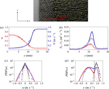
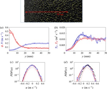
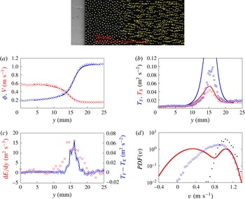
In figure 4(a), we plot the longitudinal mean velocity
 $V$
and the volume fraction
 $\unicode[STIX]{x1D719}$
of the granular gas for a Mach number
 $Ma=6$
in the reference frame of the front. The mean velocity and the volume fraction profiles both show the presence of the shock front. The mean velocity, equal to
 $V_{1}$
far from the front, decreases to a value close to zero near the obstacle. Note that, although the mean velocity decreases as in molecular gases, the low value reached does not respect the Rankine–Hugoniot conditions. The volume fraction value, equal to
 $\unicode[STIX]{x1D719}_{1}^{\ast }$
in the supersonic region, increases drastically to reach values near the close compact volume fraction in the subsonic region. This is the first indication that granular systems are different from molecular gases as noted above and in previous studies (Boudet et al.
Reference Boudet, Amarouchene and Kellay2008; Sirmas & Radulescu Reference Sirmas and Radulescu2015). Another observation which reinforces this aspect comes from the variation of the temperature versus distance across the shock front (figure 4
b). As in molecular gases, the longitudinal temperature goes through a maximum across the front and is different from the transverse temperature. However and contrary to molecular gases, the longitudinal and transverse temperatures
 $T_{Y}$
and
 $T_{X}$
decrease further in the shock front region and go down to values close to zero near the obstacle. The trend observed here is very similar to that observed in the simulations of Sirmas & Radulescu (Reference Sirmas and Radulescu2015). The anisotropy of temperature with
 $T_{Y}>T_{X}$
in the shock front can be understood by examining velocity distributions.
Volume fraction (circles) and velocity (diamonds) versus
 $y$
(a) and transverse (circles) and longitudinal (diamonds) temperatures measurements (b) in the reference frame of the front obtained for
 $Ma=6$
and
 $\unicode[STIX]{x1D719}_{1}^{\ast }=0.07$
. The signals are averaged over
 $0.1$
s. The supersonic flow is located in the region
 $y>15~\text{mm}$
. The curves (solid lines) are given by the resolution of inelastic bimodal model with a shock width
 $L=1~\text{mm}$
and
 $k=4$
. Photo: an instantaneous image of a granular flow which shows the increase in the number of particles induced by the displacement of the obstacle (grey area). The red arrow represents the region where the measurements displayed in the figures are carried out. The yellow arrows give the velocity of each particle in the reference frame of the front. Transverse (c) and longitudinal (d) velocity distributions measured at
 $y=12~\text{mm}$
(blue circles) and
 $y=20~\text{mm}$
(black plain circles). The solid red curves show the velocity distributions given by the resolution of the inelastic bimodal model; the distributions
 $f_{1}$
and
 $f_{2}$
for the two populations are given by dashed lines. The black vertical line shows the velocity threshold allowing the estimation of
 $\unicode[STIX]{x1D719}_{1}$
.

Volume fraction (circles) and velocity (diamonds) versus
 $y$
(a) and transverse (circles) and longitudinal (diamonds) temperatures measurements (b) in the reference frame of the front obtained for a Mach flow
 $Ma=1.3$
and a volume fraction
 $\unicode[STIX]{x1D719}_{1}^{\ast }=0.07$
. Solid lines are given by the resolution of inelastic bimodal model with a shock width
 $L=5~\text{mm}$
and
 $k=2.5$
. Photo: an instantaneous image of a granular flow. The red arrow represents the region described on the graphs. Transverse (c) and longitudinal (d) velocity distributions measured at
 $y=18~\text{mm}$
(blue symbols) and in the bath (black plain symbols). The red curves show the velocity distributions given by the resolution of inelastic bimodal model.

The longitudinal velocity distribution
 $PDF(v)$
in the front, clearly shows a two peak structure while the distribution in the supersonic region is single peaked with a smaller width (figure 4
d). This bimodal nature, illustrated in figure 4(d) at a location corresponding to the position of the maximum in temperature anisotropy, makes for a much larger width of the distribution and therefore the temperature along the longitudinal direction. Far from the front, where the temperature is isotropic (see figure 4
b) the velocity distributions along both axes are superimposed as the temperature becomes isotropic in these two cases.
5.2 Supersonic regime for
$Ma=1.3$

An interesting aspect of our system is the possibility to approach the subsonic–supersonic transition. Macroscopic quantities for the granular gas are plotted for
 $Ma=1.3$
in figure 5(a,b). Similarly to the large Mach number regime in figure 5(a), density and mean velocity profiles show a clear transition from their initial values in the initial supersonic gas to their final values in the subsonic region. However there are some notable differences compared to the hypersonic regime: the maxima of the temperatures along the longitudinal and transverse directions are lower and the extent of the anisotropic region is wider. Both features are found in molecular gases upon approaching
 $Ma=1$
, indicating an increase of the shock width (Alsmeyer Reference Alsmeyer1976). The distribution of longitudinal velocities does not show a clear bimodality as shown in figure 5(d) and observed in molecular gas (Muntz & Harnett Reference Muntz and Harnett1969). Note that the velocity distributions in the supersonic and shock front regions are almost identical for the transverse component (figure 5
c). The longitudinal component in the front is slightly wider (figure 5
d). This quasi-absence of the bimodal nature of the distributions has also been found in gases according to the Mott-Smith model and the Rankine–Hugoniot conditions as discussed in § 2.
5.3 Subsonic regime for
$Ma=0.5$

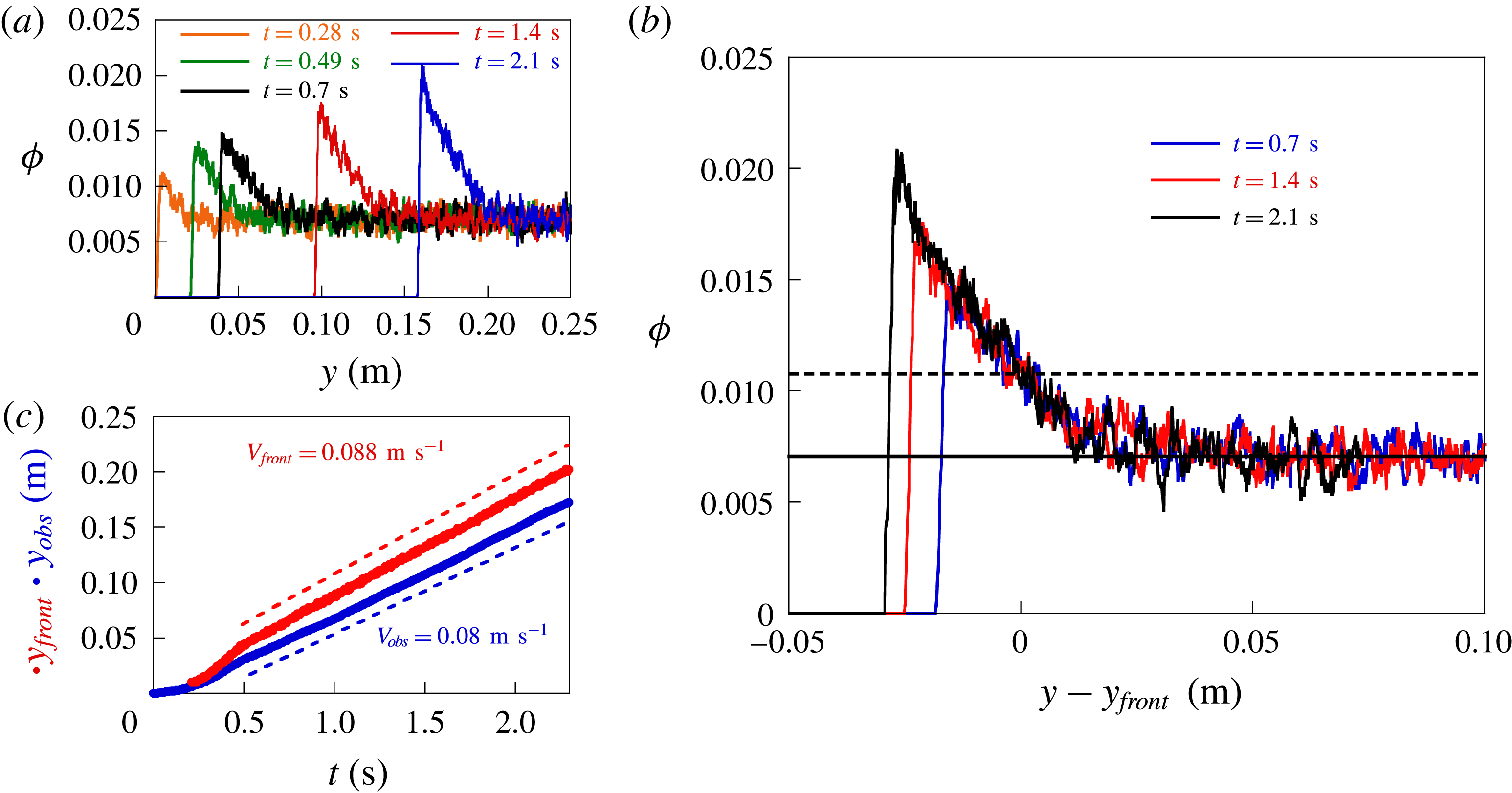
When the obstacle velocity is reduced further, we observe a stationary front moving at subsonic velocity. To check that the front propagation reaches a stationary state, we have plotted the volume fraction across the front at different times in figure 6(a). As the obstacle moves forward, steel beads accumulate and the maximum of volume fraction increases continuously. We obtain the front displacement by tracking the position
 $y_{front}$
defined by the value
 $\unicode[STIX]{x1D719}(y_{front})=0.11$
for the volume fraction. Like the obstacle velocity, the front velocity
 $V_{front}=dy_{front}/dt$
becomes constant after a transient (see figure 6
c). Despite this accumulation, we observe that all the volume fraction profiles can be superimposed (see figure 6
b). The profile shape remains a constant shape during propagation. This constant shape and front velocity allow us to conclude that the front is stationary, which has no equivalent in molecular gases.
(a) Volume fraction profiles in the reference frame of the laboratory (a) and in the reference frame of the front (b).
 $y_{front}$
corresponds to the position where a fixed value
 $\unicode[STIX]{x1D719}(y_{front})=0.11$
of volume fraction is reached (in dashed line). (c) Obstacle and front positions during obstacle propagation. The dashed line indicate a linear adjustment and the constant velocities obtained. The volume fraction is
 $\unicode[STIX]{x1D719}_{1}^{\ast }=0.07$
and the free stream Mach number
 $Ma=0.5$
.

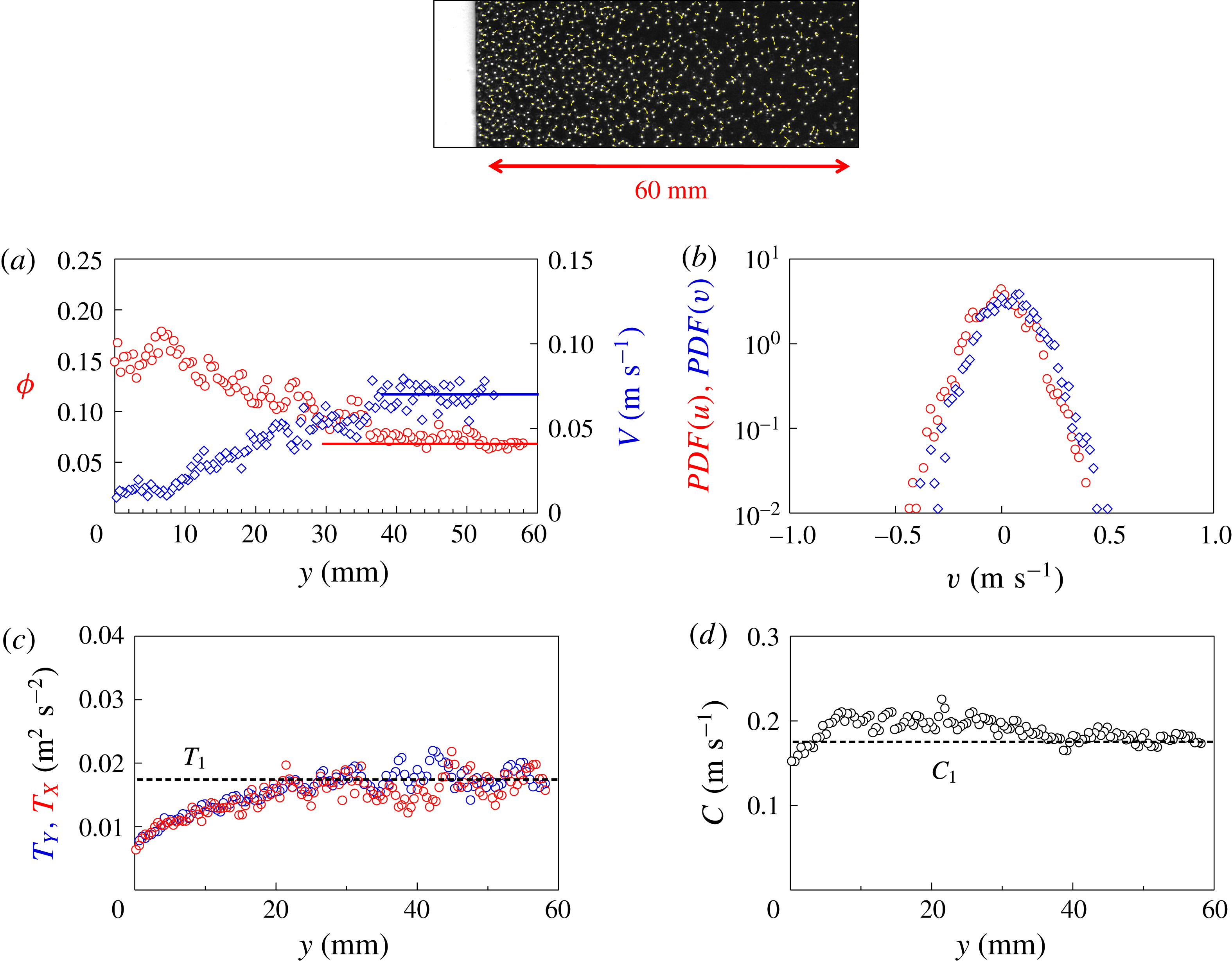
The volume fraction, mean velocity and temperature profiles are obtained by using a temporal average and plotted in figure 7 for a Mach number
 $Ma=0.5$
. The variation of the velocity and the volume fraction show a slight decrease and a slight increase near the obstacle respectively. It is interesting to note that on the one hand the temperatures do not go through a maximum but seem to have a plateau far away from the obstacle and decrease continuously upon its approach. On the other hand, there is no difference between the two temperatures. The PDFs of the velocity also show that the two components are roughly isotropic ruling out a temperature anisotropy.
Volume fraction (circles) and velocity (diamonds) versus
 $y$
(a) and transverse (circles) and longitudinal (diamonds) temperatures measurements (b) in the reference frame of the front obtained for a Mach flow
 $Ma=0.5$
and a volume fraction
 $\unicode[STIX]{x1D719}_{1}^{\ast }=0.07$
. The horizontal lines indicate the corresponding values in the region far from the obstacle. (c) Velocity distributions obtained at
 $y=15~\text{mm}$
. Photo: an instantaneous image of a granular flow. (d) Local speed of sound
 $C_{1}$
calculated from the experimental measurements of
 $\unicode[STIX]{x1D719}$
and
 $T$
with the equation (3.6). The red arrow represents the region described on the graphs.

As expected, these elements indicate the absence of a shock front at Mach numbers smaller than 1. Using the criterion of temperature anisotropy and analysing the different experiments carried out, it appears that there is presence of a shock front only if
 $Ma>1\pm 0.2$
(Vilquin Reference Vilquin2015). This is an indirect measurement of the sound speed in our granular gas. And the value extracted for the sound velocity is consistent with those provided by the granular kinetic theory (see (3.6)).
To our knowledge, the stationary state observed here has no equivalent in molecular gases. In such gases, a piston produces a compression and induces a temperature increase leading to an increase of the speed of sound near the obstacle. The velocity of compression waves emitted decreases as they move away from the obstacle (Landau & Lifchitz Reference Landau and Lifchitz1971). The first emitted compression waves are caught by those emitted later with higher velocities and the front gradually stiffens. After this unsteady stage, a stationary and supersonic shock front emerges. However, we observe a stationary state in granular gases. In these gases, compression induces a temperature decrease and we observe in figure 7(d) that sound speed slightly increases across the front without stiffening of the front (see figure 6 b). One possible explanation might be that perturbations due to gas compression are slowed down by friction between the top and bottom walls and attenuated by dissipation due to inelastic collisions.
5.4 A dissipative bimodal description
In order to understand this phenomenology for different Mach numbers, we have solved numerically the inelastic bimodal model as explained in § 3. The model, including the closure relation for
 $\unicode[STIX]{x1D719}_{1}$
(see (3.11)) and the dissipation term (see (3.15)), provides a way to obtain the macroscopic properties
 $\unicode[STIX]{x1D719}_{1}$
,
 $V_{1}$
,
 $T_{1}$
for the supersonic flow and
 $\unicode[STIX]{x1D719}_{2}$
,
 $V_{2}$
,
 $T_{2}$
for the subsonic flow, versus the position
 $y$
in the shock front. It also allows us to calculate the average quantities of the flow
 $\unicode[STIX]{x1D719}$
,
 $V$
,
 $T_{X}$
and
 $T_{Y}$
. The numerical calculation requires two adjustable parameters:
 $L$
which is the thickness or the width of the shock front and
 $k$
which is a measure of the dissipation. Details about the determination of these two parameters are provided in appendix A.
The results of our calculations are shown as continuous lines in figure 4 with
 $L=1$
and
 $k=4$
for
 $Ma=6$
, which is representative of our large Mach number experiments. There is a very good agreement for the volume fraction
 $\unicode[STIX]{x1D719}$
, the mean longitudinal velocity
 $V$
and the transverse temperature
 $T_{X}$
. For the longitudinal temperature
 $T_{Y}$
, the functional shape is consistent with experiments, but the maximum value is overestimated by a factor of
 $1.5$
. The shock width
 $L$
is found equal to 1 mm for this Mach number. This value is consistent with that obtained independently from the volume fraction
 $\unicode[STIX]{x1D719}_{1}(y)$
of the supersonic flow as shown in figure 10(b). The analysis of all the experiments carried out at large Mach numbers (
 $2.5<Ma<13$
) show similar results: a very good agreement for
 $T_{X}$
,
 $V$
and
 $\unicode[STIX]{x1D719}$
and an overestimation of the maxima of
 $T_{Y}$
.
This difference can be understood by constructing the velocity distribution with the macroscopic quantities
 $\unicode[STIX]{x1D719}_{1}$
,
 $V_{1}$
,
 $T_{1}$
,
 $\unicode[STIX]{x1D719}_{2}$
,
 $V_{2}$
,
 $T_{2}$
obtained from our dissipative bimodal description (see figure 4
c,d) similarly to the Mott-Smith model in molecular gases. In our case, Gaussian distributions are used for convenience but in the experiments the distributions are not strictly Gaussian. We will however continue using the Gaussian form for simplicity. Note that in the front region the bimodal distribution describes correctly the distributions of transverse velocities (see continuous lines in figure 4
c), but relatively poorly the measured distributions of longitudinal velocities (see figure 4
d). One possible reason for such a discrepancy is related to the presence of a surplus of intermediate particles. Indeed the measured distributions show a surplus at intermediate speeds at the expense of the peak of subsonic particles in molecular gases (Pham-Van-Diep et al.
Reference Pham-Van-Diep, Erwin and Muntz1989) and in granular gases (Boudet et al.
Reference Boudet, Amarouchene and Kellay2008; Vilquin et al.
Reference Vilquin, Boudet and Kellay2016), which is consistent with a lower measured temperature. The bimodal description, although better than the hydrodynamic description, is not complete and needs an additional population as shown in Vilquin et al. (Reference Vilquin, Boudet and Kellay2016). These intermediate particles could be the main cause of the overestimation of
 $T_{Y}$
by the model.
The inelastic bimodal model can also be solved for supersonic regime at lower Mach numbers. The results are plotted with
 $L=5$
and
 $k=2.5$
for
 $Ma=1.3$
in figure 5(a,b) as continuous lines. The model is in agreement for the measurements including the longitudinal temperature
 $T_{Y}$
, which is not the case at large Mach numbers as shown above. It should be noted that the longitudinal velocity distributions are in this case well described by the model (figure 5
c,d). This is also observed in gases for low Mach numbers for which the Mott-Smith model describes the distributions of longitudinal speeds very well. For these low Mach numbers, the presence of intermediate particles is less important.
Note here that the dissipation term used has an unknown parameter
 $k$
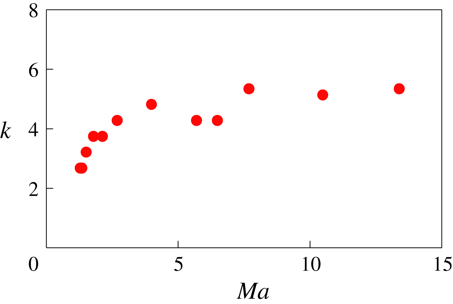
. By inspecting all the experiments at different Mach numbers, we find a value of
 $k$
that is approximately 3 for low Mach numbers and increases up to values of
 $k=5\pm 1$
for higher Mach numbers as shown in figure 8. These values of
 $k$
are larger than those predicted for the granular inelastic dissipation where
 $k=1$
. A few elements must be reported. First, contrary to our model, the restitution coefficient
 $r$
may have a velocity dependence (Lifshitz & Kolsky Reference Lifshitz and Kolsky1964) and decreases for collisions at high velocities. The consequence of such a dependence is that the value of
 $r$
could be smaller than 0.95 for high Mach number experiments which is in agreement with high
 $k$
values shown in figure 8. Secondly, in a real granular medium, there is frictional dissipation. It is an additional source of dissipation which is not considered in the model. The last point is that theoretical dissipation is calculated for a three-dimensional environment. In these experiments, the granular material is confined and vibrated. So the number of collisions between grains and thus the dissipation could probably be underestimated.
Values of dissipation coefficient
 $k$
used to adjust the inelastic bimodal model with experimental measurements versus free stream Mach number
 $Ma$
for an initial volume fraction
 $\unicode[STIX]{x1D719}_{1}^{\ast }=0.07$
.

6 Discussion
The results presented above show that the Mott-Smith model adapted to granular media gives a reasonable description of our experiments carried out at different Mach numbers. This model explains both the velocity and volume fraction profiles and gives a reasonable approximation to the temperature anisotropy characteristic of the shock fronts observed.
6.1 Width of the shock front
As we will see below, the outcome of this analysis is the shock front width. To summarize and discuss the results obtained in the previous part, we present in figure 9 the shock width denoted
 $L$
, deduced from our analysis using the model described above, as a function of the Mach number, from the different experiments carried out. We plot the shock width
 $L$
normalized by the mean free path
 $\unicode[STIX]{x1D706}=d/6\sqrt{2}\unicode[STIX]{x1D719}_{1}^{\ast }$
calculated in the gas in three dimensions. (There are no calculations for mean free path in a confined gas to our knowledge.)
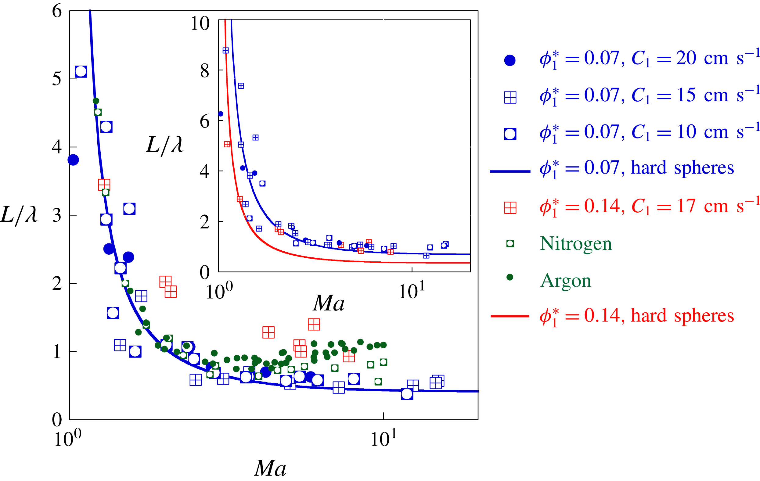
Shock width normalized by the mean free path
 $\unicode[STIX]{x1D706}=d/6\sqrt{2}\unicode[STIX]{x1D719}_{1}^{\ast }$
versus
 $Ma$
for
 $\unicode[STIX]{x1D719}_{1}^{\ast }=0.07$
and
 $C_{1}=0.1,0.15,0.2~\text{m}~\text{s}^{-1}$
(blue symbols) and
 $\unicode[STIX]{x1D719}_{1}^{\ast }=0.14$
and
 $C_{1}=0.175~\text{m}~\text{s}^{-1}$
(red symbols). The blue line gives the resolution of the Mott-Smith model for a gas of hard spheres. To compare to molecular gases, green symbols give the shock widths measured in argon and nitrogen (Alsmeyer Reference Alsmeyer1976). Inset: the shock width normalized by the bead diameter
 $d$
versus
 $Ma$
. The lines give the resolution of the Mott-Smith model for a gas of hard spheres. It should be noted that for large Mach numbers and for both volume fraction shock width becomes approximately half the size of the bead.

Let us consider first the measurements made with the initial volume fraction
 $\unicode[STIX]{x1D719}_{1}^{\ast }=0.07$
. The shock width
 $L$
clearly shows a saturation for Mach numbers between 3 and 13. At lower Mach numbers, the width
 $L$
increases as the Mach number goes to 1. This behaviour is characteristic of shock fronts in molecular gases as illustrated in the same figure where measurements in gases are shown for argon and nitrogen (Alsmeyer Reference Alsmeyer1976). That the width of the shock front increases near Mach 1 is reminiscent of the fact that the shock is becoming shallower as the speed of sound is approached from above. The variation of the width with Mach number seems to follow the Mott-Smith prediction quite reasonably. We recall here that the Mott-Smith prediction uses the bimodal nature of the velocity distributions, considers hard spheres with elastic interactions and does not consider dissipation. Therefore the fact that the widths we extract from our analysis follow this prediction is in itself surprising. To our knowledge, these are the first measurements of shock front width for a wide range of Mach numbers in granular gases.
We mention above that the energy dissipation seems to have a little influence on the
 $L$
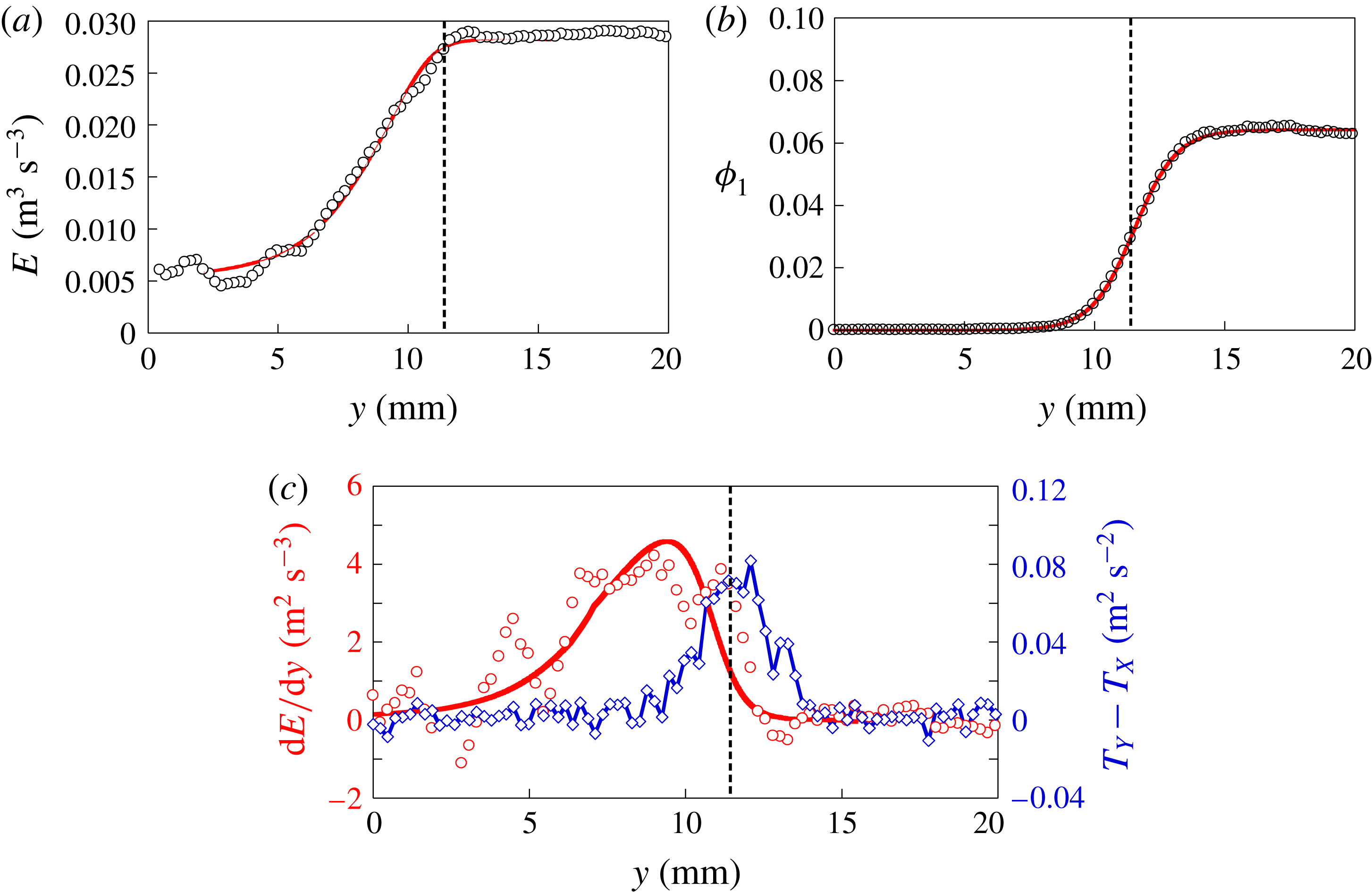
values of the shock width while it affects the temperature and density variations. A possible explanation is related to the spatial localization of the dissipation. We examine the spatial variation of the energy and pressure flux
 $E$
, defined in equation (3.10). The flux
 $E$
is evaluated using experimental data and its variation is shown in figure 10(a) along with the variation of the density of the supersonic population (see figure 10
b). Note that this energy flux across the shock should be constant in the absence of dissipation which is not the case here. It decreases near the end of the shock front where dissipation becomes important. We plot the derivative
 $dE/dy$
of this term, which is equivalent to the dissipation
 $\unicode[STIX]{x1D6E4}$
, along with the temperature anisotropy in figure 10(c). Note that the peak of the dissipation is located slightly to the left of the maximum of the temperature difference
 $T_{Y}-T_{X}$
. It shows that the dissipation remains small at the shock front and becomes important only when the supersonic particles have significantly decreased. The shock width is basically determined before the dissipation becomes important. The value of the shock width, therefore, has a low sensitivity to the presence of dissipation.
(a) The profile of the energy and pressure flux
 $E$
estimated by equation (3.10). The red curve gives the inelastic bimodal model. (b) The volume fraction
 $\unicode[STIX]{x1D719}_{1}$
of supersonic particles; the red curve is a fit of the analytic form given by equation (3.11) with
 $L=1~\text{mm}$
. (c) Derivative of the energy flux
 $E$
from experimental measurements (red circles) and the model (red line) plotted in (a), and temperature difference
 $T_{Y}-T_{X}$
(blue diamonds) as function of
 $y$
. Note that the maxima of each curve do not coincide. The flow properties are a Mach number
 $Ma=6$
and a volume fraction
 $\unicode[STIX]{x1D719}_{1}^{\ast }=0.07$
.

Volume fraction (circles) and velocity (diamonds) versus
 $y$
(a) and transverse (circles) and longitudinal (diamonds) temperatures measurements (b) in the reference frame of the front obtained for a Mach flow
 $Ma=6$
and a volume fraction
 $\unicode[STIX]{x1D719}_{1}^{\ast }=0.14$
. (c) Derivative of the energy flux
 $E$
from experimental measurements (red circles), and temperature difference
 $T_{Y}-T_{X}$
(blue diamonds) as function of
 $y$
. Note that the maxima of each curve do coincide contrary to the previous case
 $\unicode[STIX]{x1D719}_{1}^{\ast }=0.07$
plotted in figure 10. (d) Longitudinal velocity distribution in the bath (black symbols) and near the maxima of the temperature anisotropy (blue symbols). The red curves show the velocity distributions given by the resolution of inelastic bimodal model with
 $k=5$
.

Note that we neglected the dissipation term
 $\unicode[STIX]{x1D6E4}_{1,2}$
(3.13), due to inelastic collisions between supersonic and subsonic particles. The ratio
 $\unicode[STIX]{x1D6E4}_{2,2}/\unicode[STIX]{x1D6E4}_{1,2}\propto \unicode[STIX]{x1D719}_{2}/\unicode[STIX]{x1D719}_{1}$
, where
 $\unicode[STIX]{x1D6E4}_{2,2}$
(3.12) is the dissipation term due to inelastic collisions between subsonic particles. Figures 10 and 4(a) show that the energy dissipation starts for a value of the supersonic volume fraction
 $\unicode[STIX]{x1D719}_{1}$
smaller compared to the subsonic volume fraction
 $\unicode[STIX]{x1D719}_{2}=\unicode[STIX]{x1D719}-\unicode[STIX]{x1D719}_{1}$
. Thus the contribution of
 $\unicode[STIX]{x1D6E4}_{1,2}$
is negligible compared to the dissipation term
 $\unicode[STIX]{x1D6E4}_{2,2}$
.
6.2 Effect of the initial volume fraction on the shock front
Let us go back to figure 9 displaying the shock width
 $L$
versus the Mach number
 $Ma$
. We have used different sound speeds (we control the temperature
 $T_{1}$
by changing the characteristics of the vibration) and we have also tested another initial volume fraction
 $\unicode[STIX]{x1D719}_{1}^{\ast }$
to examine the validity of our model. For the higher volume fraction
 $\unicode[STIX]{x1D719}_{1}^{\ast }=0.14$
, the widths seem to deviate from the Mott-Smith prediction for elastic spheres. As mentioned above, the dissipation and the temperature anisotropy are spatially separated (as shown in figure 10) for the dilute case
 $\unicode[STIX]{x1D719}_{1}^{\ast }=0.07$
. However, this may no longer be the case for the higher volume fraction. In order to examine this in detail, we plot in figure 11, the mean velocity, the temperatures and the volume fraction profiles for
 $Ma=6$
and
 $\unicode[STIX]{x1D719}_{1}^{\ast }=0.14$
. The overall picture is similar to that observed at large Mach numbers above (see figure 4 with
 $Ma=6$
and
 $\unicode[STIX]{x1D719}_{1}^{\ast }=0.07$
) as both the density and the velocity show a clear transition from their initial values in the supersonic regime to their final values in the subsonic region. However there are some notable differences; the maxima of the temperatures along the longitudinal and transverse directions are lower for the higher volume fraction. The distribution of longitudinal velocities does not show a clear bimodality as seen in figure 11. Furthermore, the inelastic bimodal model with
 $k=5$
and
 $L=1~\text{mm}$
(see the continuous line in figure 11) shows an important disagreement for the temperature profiles, notably for
 $T_{X}$
which was not the case at lower volume fraction. Two explanations can be put forth. First, the main hypothesis of the model is that in the shock front the velocity distributions are bimodal. The experimental results do not show clearly a bimodality for the high density case. Thus, the description with two populations is perhaps not valid. Possibly, this is due to the nature of the shocks between steel beads. An inspection of videos of the experiments shows that in the area of the shock wave, many shocks are not binary as a particle may collide with a pair of particles simultaneously for example or with small clusters of particles. Our model, derived from kinetic theory is only valid for dilute granular flows with binary collisions and not for dense flows. Second, the spatial separation between the peak of the dissipation and the maximum of temperature anisotropy and therefore the shock front are not clearly visible in figure 11. These observations, and perhaps other effects for the higher volume fraction (such as the finite size effects where the mean free path becomes comparable to the particle size, see inset in figure 9), clearly point to the limitations of the approach developed here and the requirement for additional work. Nevertheless and for the dilute case, the shock fronts turn out to be well described by the approach proposed here and the width of the shock follows the simple Mott-Smith model for elastic hard spheres.
7 Conclusion
A moving planar obstacle in a vibrated granular gas creates a shock front which moves at constant speed, controllable by the obstacle velocity. This experimental set-up can generate one-dimensional shock waves in a granular gas at the desired Mach number. In the shock fronts, the velocity distributions show a structure with two peaks. An inelastic model of granular shock front with two populations, based on the Mott-Smith model for molecular gases is proposed and its resolution correctly reproduces the different profiles obtained experimentally and notably that of the temperature anisotropy. The few remaining disagreements observed for large Mach numbers, in particular the magnitude of the temperature anisotropy, indicate that this bimodal description is still approximate and should be expanded. One of the possible extensions is that to a three-population model as proposed recently (Vilquin et al. Reference Vilquin, Boudet and Kellay2016). An important result concerns the width of the shock front. This width is found experimentally to be very close to that of a gas of hard spheres, and this for all Mach numbers studied. This agreement can be explained by the weak role of the dissipation in a large part of the shock front.
Acknowledgements
We thank E. Maillard from the Machine shop for help with the experimental set-up. A.V. was supported by a fellowship of the University of Bordeaux.
Appendix Numerical resolution
In this section, we present the numerical method to solve the inelastic bimodal model described in § 3. With the two additional ingredients, the dissipation term
 $\unicode[STIX]{x1D6E4}$
(3.15) and the closure relation for the volume fraction
 $\unicode[STIX]{x1D719}_{1}(y)$
(3.11), we numerically solved the hydrodynamic equations (3.8), (3.9), (3.10) with a Euler method. For a given spatial position
 $y$
, equations are:
 $$\begin{eqnarray}\displaystyle & \displaystyle \unicode[STIX]{x1D719}_{1}V_{1}+\unicode[STIX]{x1D719}_{2}V_{2}=M, & \displaystyle\end{eqnarray}$$
 $$\begin{eqnarray}\displaystyle & \displaystyle \unicode[STIX]{x1D719}_{1}(V_{1}^{2}+\unicode[STIX]{x1D712}_{1}T_{1})+\unicode[STIX]{x1D719}_{2}(V_{2}^{2}+\unicode[STIX]{x1D712}_{2}T_{2})=P, & \displaystyle\end{eqnarray}$$
 $$\begin{eqnarray}\displaystyle & \displaystyle {\textstyle \frac{1}{2}}\unicode[STIX]{x1D719}_{1}V_{1}(V_{1}^{2}+(n+2\unicode[STIX]{x1D712}_{1})T_{1})+{\textstyle \frac{1}{2}}\unicode[STIX]{x1D719}_{2}V_{2}(V_{2}^{2}+(n+2\unicode[STIX]{x1D712}_{2})T_{2})=E. & \displaystyle\end{eqnarray}$$
For greater clarity, we denote
 $\unicode[STIX]{x1D712}_{i}=\unicode[STIX]{x1D712}(\unicode[STIX]{x1D719}_{i})$
where
 $\unicode[STIX]{x1D712}(\unicode[STIX]{x1D719})$
is given by the equation (3.4). The initial values of the flux
 $M$
,
 $P$
,
 $E$
are given by the supersonic gas properties far from the shock front (
 $y\rightarrow +\infty$
). We assume the supersonic volume fraction
 $\unicode[STIX]{x1D719}_{1}$
is given by the closure equation (3.11). The equations can be rewritten:
 $$\begin{eqnarray}\displaystyle & \displaystyle \unicode[STIX]{x1D719}_{2}V_{2}=\tilde{M}=M-\unicode[STIX]{x1D719}_{1}V_{1}, & \displaystyle\end{eqnarray}$$
 $$\begin{eqnarray}\displaystyle & \displaystyle \unicode[STIX]{x1D719}_{2}(V_{2}^{2}+\unicode[STIX]{x1D712}_{2}T_{2})=\tilde{P}=P-\unicode[STIX]{x1D719}_{1}(V_{1}^{2}+\unicode[STIX]{x1D712}_{1}T_{1}), & \displaystyle\end{eqnarray}$$
 $$\begin{eqnarray}\displaystyle & \displaystyle \unicode[STIX]{x1D719}_{2}V_{2}(V_{2}^{2}+(n+2\unicode[STIX]{x1D712}_{2})T_{2})=\tilde{E}=2E-\unicode[STIX]{x1D719}_{1}V_{1}(V_{1}^{2}+(n+2\unicode[STIX]{x1D712}_{1})T_{1}). & \displaystyle\end{eqnarray}$$
We choose an initial value
 $y_{1}$
where the supersonic gas volume fraction
 $\unicode[STIX]{x1D719}_{1}$
is very close to
 $\unicode[STIX]{x1D719}_{1}^{\ast }$
. We assume for
 $y=y_{1}$
:
 $$\begin{eqnarray}\displaystyle \left.\begin{array}{@{}c@{}}\displaystyle M(y_{1})\approx M(y\rightarrow +\infty )=\unicode[STIX]{x1D719}_{1}^{\infty }V_{1},\\ \displaystyle P(y_{1})\approx P(y\rightarrow +\infty )=\unicode[STIX]{x1D719}_{1}^{\infty }(V_{1}^{2}+\unicode[STIX]{x1D712}(\unicode[STIX]{x1D719}_{1}^{\infty })T_{1}),\\ \displaystyle E(y_{1})\approx E(y\rightarrow +\infty )={\textstyle \frac{1}{2}}\unicode[STIX]{x1D719}_{1}^{\infty }V_{1}(V_{1}^{2}+(n+2\unicode[STIX]{x1D712}(\unicode[STIX]{x1D719}_{1}^{\infty }))T_{1}),\\ \displaystyle \unicode[STIX]{x1D712}_{2}(y_{1})\approx \unicode[STIX]{x1D712}_{2}(y\rightarrow +\infty )=1.\end{array}\right\} & & \displaystyle\end{eqnarray}$$
From these assumptions, the equations (A 4), (A 5), (A 6) can be solved to obtain subsonic gas properties
 $\unicode[STIX]{x1D719}_{2}$
,
 $V_{2}$
,
 $T_{2}$
for
 $y=y_{1}$
. In the same way, for the next value
 $y_{2}=y_{1}+\unicode[STIX]{x1D6FF}y$
with a very small value
 $\unicode[STIX]{x1D6FF}y$
, mass and momentum flux keep the same values. The energy flux vary because of dissipation:
 $E(y_{2})=E(y_{1})+\unicode[STIX]{x1D6E4}\unicode[STIX]{x1D6FF}y$
, and we assume
 $\unicode[STIX]{x1D712}_{2}(y_{2})=\unicode[STIX]{x1D712}_{2}(y_{1})$
for
 $\unicode[STIX]{x1D6FF}y$
sufficiently small. Properties of the subsonic gas are calculated step by step across the shock front. This method is robust without convergence problems.
This numeric resolution requires two input parameters: the shock width
 $L$
and a dissipation coefficient
 $k$
. We solve the system with different values
 $(L;k)$
to obtain the best agreement with experimental measurements. The numeric solving shows that the
 $L$
value is mainly given by temperature difference
 $T_{Y}-T_{X}$
as discussed in § 3.3.
To compare with experimental measurements, we calculated the total macroscopic quantities:
 $$\begin{eqnarray}\displaystyle \left.\begin{array}{@{}c@{}}\displaystyle \unicode[STIX]{x1D719}=\unicode[STIX]{x1D719}_{1}+\unicode[STIX]{x1D719}_{2},\quad V=\frac{\unicode[STIX]{x1D719}_{1}V_{1}+\unicode[STIX]{x1D719}_{2}V_{2}}{\unicode[STIX]{x1D719}},\\ \displaystyle T_{X}=\frac{\unicode[STIX]{x1D719}_{1}T_{1}+\unicode[STIX]{x1D719}_{2}T_{2}}{\unicode[STIX]{x1D719}},\quad T_{Y}=\frac{\unicode[STIX]{x1D719}_{1}(T_{1}+V_{1}^{2})+\unicode[STIX]{x1D719}_{2}(T_{2}+V_{2}^{2})}{\unicode[STIX]{x1D719}}-V_{Y}^{2},\end{array}\right\} & & \displaystyle\end{eqnarray}$$
where
 $\unicode[STIX]{x1D719}$
,
 $V$
,
 $T_{X}$
,
 $T_{Y}$
are respectively the total volume fraction, the longitudinal mean velocity, the transverse and longitudinal temperatures of the granular gas in the shock front. Results are shown in § 5.