1. Introduction
When a shock wave interacts with the perturbation interface between two fluids with different densities, the disparity between the pressure and density gradients leads to the generation and accumulation of oblique vorticity at the interface (Brouillette Reference Brouillette2002). These vortices accelerate the growth of interface perturbations, leading to the penetration of light (heavy) fluids into heavy (light) fluids, and the formation of bubble (spike) mixing zones. This type of instability is called the Richtmyer–Meshkov (RM) instability, first predicted theoretically by Richtmyer (Reference Richtmyer1960) and then confirmed by Meshkov (Reference Meshkov1969) in shock-tube experiments. Subsequent experiments further determined that for multi-mode initial interface perturbations, this instability rapidly transitioned to turbulent mixing. In addition, if an incident shock wave is reflected and reshocks a previously developed mixing zone, then it exacerbates the development of turbulence. This phenomenon is the reshocked RM turbulent mixing, investigated in the present study (Mikaelian Reference Mikaelian1989). The problem of reshock in RM instability was first introduced and systematically examined by Mikaelian (Reference Mikaelian1985). Reshock RM turbulent mixing is widely observed in various natural phenomena and used in engineering applications, including supernova explosions (Shimoda et al. Reference Shimoda, Inoue, Ohira, Yamazaki, Bamba and Vink2015), aerospace engines (Yang, Zhang & Sharp Reference Yang, Zhang and Sharp1994) and inertial confinement fusion (Lindl, McCrory & Campbell Reference Lindl, McCrory and Campbell1992). The study of this process holds significant scientific and engineering value (Zhou et al. Reference Zhou, Williams, Ramaprabhu, Groom and Attal2021, Reference Zhou, Clark, Clark, Gail Glendinning, Aaron Skinner, Huntington, Hurricane, Dimits and Remington2019; Ni, Zeng & Zhang Reference Ni, Zeng and Zhang2023; Zhang et al. Reference Zhang and Ni2023).
As the most fundamental global quantity, mixing width has been widely used to characterize the evolution of reshock RM mixing. The mixing width is usually defined as the distance between the average volume fractions
 $1\,\%$
and
 $99\,\%$
(or
 $5\,\%$
and
 $95\,\%$
) (Zhou Reference Zhou2017). According to the evolution characteristics of the mixing width, reshock RM turbulent mixing can be classified into three stages. The first stage involves the classical RM instability and turbulent mixing induced by the incident shock wave interacting with the interface perturbations. At this stage, the evolution of the mixing width
 $h$
over time
 $t$
transitions from linear growth in the early time
 $h \propto t$
to power-law growth in the later phase,
 $h \propto t^{\theta}$
, where
 $\theta \in (0,1)$
is the power-law growth index (Meyer et al. Reference Meyer and Blewett1972; Youngs Reference Youngs2004; Thornber et al. Reference Thornber, Drikakis, Youngs and Williams2010; Reese et al. Reference Reese, Ames, Noble, Oakley, Rothamer and Bonazza2018). The second stage involves shock-induced compression of the mixing zone and intensified turbulent mixing caused by the shock. At this stage, the mixing width first narrows owing to shock-induced compression (Thornber et al. Reference Thornber, Drikakis, Youngs and Williams2012), subsequently undergoing a process similar to the evolution of the mixing width in the first stage (Mikaelian Reference Mikaelian2011). The third stage involves complex interactions between the mixing zone and multiple wave systems caused by transmitted and reflected waves. At this stage, the evolution of the mixing width is extremely complex, and related research remains primarily at the qualitative level (Li et al. Reference Li, He, Zhang and Tian2019). No prior quantitative theoretical model could predict the evolution of the mixing width at this stage.
Presently, the academic community has a relatively deep understanding of the first stages of RM turbulent mixing. Specifically, a theoretical model is established for the evolution of this stage. In the early stages of this stage, perturbations of various wavelengths maintain relatively independent linear growth according to Richtmyer’s impulsive model (Richtmyer Reference Richtmyer1960):
 \begin{equation} \frac {{\rm d}a}{{\rm d}t}=k\Delta u\, a^{+}_0 \! A^{+}, \end{equation}
where
 $t$
is the time,
 $k\equiv 2\unicode{x03C0} /\lambda$
is the wavenumber,
 $a_0$
is the initial perturbation amplitude, superscript
 $+$
represents the instant immediately after the shock, the Atwood number
 $A^{+}\equiv (\rho _{2}^{+}-\rho _1^{+})/(\rho _{2}^{+}+\rho _1^{+})$
is the dimensionless density ratio defined by the light fluid density
 $\rho _1^{+}$
and heavy fluid density
 $\rho _{2}^{+}$
after the shock, and
 $\Delta u$
is the change in the interface velocity resulting from the passage of the shock. In the subsequent transitional period, short-wavelength perturbations generally attain linear saturation and enter the merger stage, where long-wavelength perturbations begin to form and dominate the growth of the mixing region. During this period, the merger of neighbouring bubbles facilitates the formation of larger-scale structures, causing perturbations to shift towards the
 $h \propto t^{\theta}$
power-law growth mode (Thornber et al. Reference Thornber2017). Simultaneously, the large-scale structure breaks down into small-scale vortices, and the flow transitions to fully developed turbulent mixing. At this stage, the bubble and spike structures cannot be distinguished, culminating in a turbulent mixing zone. Before the arrival of the second shock, the mixing width continues to exhibit steady power-law growth (Groom et al. Reference Groom and Thornber2020). Typically, because of the interactions among irregular multi-mode perturbations, the linear and transitional phases are relatively short, and the mixing quickly enters the fully developed turbulent mixing stage with power-law growth. Extensive experimental studies have demonstrated that the evolution of this stage depends significantly on the initial perturbation characteristics. Specifically, under short-wave perturbations, the evolution of the mixing width
 $h$
with time
 $t$
adheres to the
 $h \propto t^{\theta}$
and
 $\theta \approx 0.25$
universal power-law relationships (Dimonte et al. Reference Dimonte and Schneider2000; Prasad et al. Reference Prasad, Rasheed, Kumar and Sturtevant2000; Thornber et al. Reference Jacobs, Krivets, Tsiklashvili and Likhachev2012, Reference Li, He, Zhang and Tian2017; Thornber Reference Thornber2016). In contrast, the evolution of the mixing width under long-wave perturbations displays characteristics without a fixed power-law exponent, which is significantly influenced by the perturbation mode but generally follows
 $\theta \gt 0.25$
(Dimonte, Frerking & Schneider Reference Dimonte, Frerking and Schneider1995, Reference Dimonte and Schneider1997; Groom et al. Reference Groom and Thornber2020; Weber et al. Reference Weber, Haehn, Oakley, Rothamer and Bonazza2012, Reference Weber, Haehn, Oakley, Rothamer and Bonazza2014; Mohaghar et al. Reference Ni, Zeng and Zhang2017, Reference Pascoe, Groom, Youngs and Thornber2019; Zhuo Reference Zhuo and Shi2007). Recently, the extended multi-mode wave-packet model developed by Dimonte et al. (Reference Dimonte, Nagori, Ramaprabhu and Boureima2024), incorporating dynamic saturation and logarithmic growth, has successfully described the transition from linear to nonlinear power-law growth in the RM instability with broadband perturbations, demonstrating its validity across a wide range of parameters.
In the second stage of reshock RM turbulent mixing, the reshock not only deposits additional vorticity but also alters the turbulent structure within the mixing zone, thereby enhancing the extent of turbulent mixing (Hill, Pantano & Pullin Reference Hill, Pantano and Pullin2006). This transformation causes the evolution pattern of the mixing width to shift from
 $h \propto t^{\theta}$
power-law growth before reshocking to
 $h \propto t$
linear growth after reshocking. In the absence of disturbances from other wave systems, the mixing evolution is expected to eventually achieve self-similar power-law growth. Ferguson and Jacobs (Reference Ferguson and Jacobs2024) dual-driver shock tube experiments reveal that the shock-to-reshock time interval significantly influences both the energy spectrum characteristics and anisotropy evolution in turbulent mixing layers. While the shock arrival sequence (heavy/light gas precedence) shows no significant impact on mixing layer growth rate, it induces measurable differences in turbulent kinetic energy (TKE) decay rates. These findings highlight the complexity of energy dissipation mechanisms in reshocked RM instability. To quantify the growth of the mixing width after reshocking, Mikaelian (Reference Mikaelian2011) developed the algebraic model
 \begin{equation} \begin{cases} \textit{linear stage} \quad \quad \ \; h=h_0^{+}+C_MA^{+}\,\Delta u\,t,& t\leqslant t^{*},\\[4pt] \textit{nonlinear stage} \quad h=h^{*}\left [1+\dot {h}^{*}\theta ^{-1}\left (t-t^{*}\right )/h^{*}\right ]^{\theta}, & t \gt t^{*},\\[4pt] \end{cases} \end{equation}
where subscript
 $0$
represents the instant of reshock, superscript
 $+$
represents the instant immediately after the shock, and superscript
 $*$
represents the quantity corresponding to the transition instant. Here,
 $h_0^{+}$
represents the post-reshock mixing width, which is closely related to the pre-shock mixing width
 $h_0^{-}$
, shock Mach number
 $M_r$
, and the density ratio of light and heavy fluids. Also,
 $C_M\equiv 2(\alpha _b+\alpha _s)$
represents the linear growth coefficient, which is closely related to the secondary growth coefficient
 $\alpha _b$
in the bubble mixing zone, and the secondary growth coefficient
 $\alpha _s$
in the spike mixing zone of Rayleigh–Taylor (RT) turbulent mixing (Taylor Reference Taylor1950; Rayleigh Reference Rayleigh1965) caused by a light fluid accelerating heavy fluid (Youngs Reference Youngs1989; Dimonte et al. Reference Dimonte and Schneider2000). Mikaelian initially suggested that
 $C_M=0.28$
based on the RT turbulent mixing experiment conducted by Read (Reference Read1984). Here,
 $\Delta u$
represents the total change in the average velocity of the mixing zone owing to a shock, which is closely related to the reshock Mach number
 $M_r$
and density ratio of light and heavy fluids. The growth-rate scaling revealed by this model was validated through extensive experiments and numerical simulations (Vetter et al. Reference Vetter and Sturtevant1995; Erez et al. Reference Erez, Sadot, Oron, Erez, Levin, Shvarts and Ben-Dor2000; Leinov et al. Reference Leinov, Malamud, Elbaz, Levin, Ben-Dor, Shvarts and Sadot2009; Jacobs et al. Reference Jacobs, Krivets, Tsiklashvili and Likhachev2013). However, disagreements persist regarding the value of the linear growth coefficient
 $C_M$
. Recently, Sun et al. (Reference Sun, Song, Wang and Zhang2024) proposed an improved model that incorporates the influence of the growth rate prior to reshocking, and ensures the continuity of the mixing width growth rate before and after reshocking. This advancement effectively unified the determination of the linear growth coefficient under different experimental conditions. For the air–
 $\text{SF}_6$
combination, the model can be expressed as
 \begin{equation} h\left (t\right )=h_0^{+}+\left (0.28A^{+}\,\Delta u+\dot {h}_0^{-}\right )t,\quad t\leqslant t^{*}. \end{equation}
Although a piecewise algebraic model for the evolution of the mixing width before and after reshocking has been established in the aforementioned research, few studies have focused on the evolution of the mixing width during the interaction between the shock waves and mixing zones. At the instant of shock, the mixing zone is subjected to substantial compression. The mixing width post-reshock,
 $h_0^{+}$
, which serves as the initial value for (1.3), traditionally relies on experimental measurements for specific values (Leinov et al. Reference Leinov, Malamud, Elbaz, Levin, Ben-Dor, Shvarts and Sadot2009) and lacks a quantitative theoretical model for prediction. In particular, the first stage of reshock RM mixing also involves interactions between the shock wave and the initial perturbed interface. Early studies by Richtmyer showed that the amplitude of perturbations is significantly compressed by shocks, and using the perturbation amplitude post-shock ensures the validity of (1.1). By combining the geometrical relationships of the shock with the interface and theories from one-dimensional gas dynamics, Richtmyer (Reference Richtmyer1960) provided a formula to calculate the post-shock perturbation amplitude:
 \begin{equation} \frac {a_0^{+}}{a_0^{-}}=1-\frac {\Delta u}{U}, \end{equation}
where
 $U$
represents the velocity of the incident shock wave. The prerequisite for the application of (1.4) is that the perturbation wavelength and amplitude must satisfy
 $ka_0\ll 1$
, and its accuracy has been validated through extensive experimental verification. In this study, we determined that the equation yields sufficient precision when calculating the compression of the light–heavy interface caused by incident shock. However, when applied to calculate the compression of the heavy–light interface, the equation exhibits certain discrepancies, suggesting that further investigation of the interactions between shock waves and interfaces is necessary.
In this study, we defined the direct interaction process between the shock wave and perturbed interface or mixing zone as the shock compression stage. Specifically, the shock compression process begins when the shock wave enters the mixing zone, and ends when it exits. Throughout reshock RM mixing, two critical shock compression stages are involved: the impact of the incident shock wave on the initial perturbed interface, and the subsequent reshock on the formed mixing zone. If the initial condition is a light–heavy interface, then the reshock interacts with a heavy–light mixing zone, and vice versa. Although studies have recognized the importance of this stage, aside from Richtmyer’s early work, few studies have conducted in-depth studies on this topic. Recently, Li et al. (Reference Li, Tian, He and Zhang2021) proposed a general principle of mixing-width growth rate decomposition (GRD) by decomposing the flow field into an averaged field and a fluctuating field. This general principle decomposes the growth rate of the mixing width into three contributions: stretching (compression), penetration and diffusion. Simulations of the RM instability in convergent geometries indicate that the three aforementioned effects are the dominant factors influencing the growth rate of the instability (Ge et al. Reference Zhang and Ni2020, Reference Zhang, Ni, Ruan and Xie2022; Pascoe et al. Reference Pascoe, Groom, Youngs and Thornber2024). Following the GRD, this study highlights the complexity of the shock compression stage. Although Li et al. (Reference Li, Tian, He and Zhang2021) did not delve deeply into this issue, their introduction of the GRD formula provided a framework for exploring the evolution of the shock compression stage. In particular, their numerical simulations revealed that the evolution of the mixing width during the shock wave from light to heavy fluid and from heavy to light fluid was dominated by different mechanisms. These results underscore the necessity of differentiating shock compression issues into light–heavy and heavy–light types. Building upon this principle, the present study seeks to further analyse the physical mechanisms and dominant factors during the shock compression stage. The research objective is to develop a model encapsulating the mixing width evolution at this stage, and enhance our understanding of the influential factors.
This paper is structured as follows. Section 2 introduces the theoretical framework of the GRD formula and reports a detailed analysis of the processes and dominant mechanisms of the two types of shock compression scenarios. In § 3, we establish a quantitative model for the shock compression stage through independent formula stretching (compression) and penetration mechanisms. The application of theoretical models to reshock RM mixing is presented in § 4. Finally, a summary and outlook are presented in § 5.
2. Physical analysis of the shock compression process
Li et al. (Reference Li, Tian, He and Zhang2021) analysed the evolution of the flow field in turbulent mixing induced by interfacial instability by separating it into mean and fluctuating components. This approach allowed them to assess the respective contributions of these components to the growth rate of the mixing width. They proposed a GRD formula that identified three contributing mechanisms: a stretching (compression) mechanism driven by the average velocity difference between the two ends of the mixing zone, a penetration mechanism induced by velocity fluctuations of the two mixing fluids, and a diffusion mechanism resulting from molecular diffusion. In high-Reynolds-number flows with a Schmidt number near unity, the influence of the diffusion mechanism is negligible. To quantify each mechanism within the model, it is necessary to utilize the average profiles of density, velocity and mass fraction, along with the histories of average acceleration within the mixing zone. It is important to note that while this model facilitates a posteriori analysis of mixing width evolution, it is not suitable for a priori predictions.
Comparison between the DNS of growth rate evolution (red dots) and the GRD formula (black solid line), as well as the contributions from the stretching (compression) – denoted S (C) – mechanism (green dashed line) and the penetration mechanism (Penetration effect). Here,
 $t_1$
and
 $t_2$
represent the starting and ending moments of the shock compression process, respectively. The plots are of the (a) first and (b) reshock compression stages. The data correspond to the air–
 $\text{SF}_6$
scenario. All data are sourced from the available literature (Li et al. Reference Li, Tian, He and Zhang2021).

The efficacy of the GRD formula for reshock RM mixing was validated through direct numerical simulations (DNS), detailing the contributions of the stretching (compression) and penetration mechanisms throughout various stages of the mixing evolution in table IV of Li et al. (Reference Li, Tian, He and Zhang2021). From the numerical results of Li et al. (Reference Li, Tian, He and Zhang2021), a complex stage in the mixing evolution, known as the shock compression stage, was identified. Compared with the post-shock stage dominated by penetration mechanisms, the shock compression stage involves the two aforementioned mechanisms. At this stage, the stretching (compression) mechanism is significant, as mentioned in Richtmyer’s earlier work (Richtmyer Reference Richtmyer1960). However, the penetration mechanism, equally important in the shock compression stage, has not received sufficient research attention. As the shock wave propagates from the light fluid to the heavy fluid, the penetration and stretching (compression) mechanisms exert opposite effects on the growth of the mixing zones, and their contributions to the growth rate are comparable, as shown in figures 1(a) and 2(b). Conversely, as the shock wave propagates from a heavy fluid to a light fluid, the two mechanisms exert the same effect on the growth of the mixing zones; however, the contribution from the penetration mechanism is significantly smaller and almost negligible. In this scenario, the stretching (compression) mechanism dominates the evolution of the mixing width, as illustrated in figures 1(b) and 2(a). This trend highlights the critical influence of the shock direction on the development of the mixing width during the shock compression stage, underscoring the need to categorize shock compression issues into two fundamental types: light-to-heavy (light–heavy) and heavy-to-light (heavy–light). This study subsequently analyses the differences in the dominant mechanisms between these two types.
Comparison between the DNS of growth rate evolution (red dots) and the GRD formula (black solid line), as well as the contributions from the stretching (compression) mechanism (green dashed line) and the penetration mechanism (Penetration effect). Here,
 $t_1$
and
 $t_2$
represent the starting and ending moments of the shock compression process, respectively. The plots are of the (a) first and (b) reshock compression stages. The data are from the
 $\text{SF}_6$
–air scenario. All data are sourced from the available literature (Li et al. Reference Li, Tian, He and Zhang2021).

Schematic of the light–heavy shock compression problem. The thick solid line represents the interface, the thin solid line represents the shock wave, and the dashed line represents the initial interface position. Here,
 $U_r$
and
 $U_t$
are the wave speeds of the reflected and transmitted waves.
 $h^{-}$
are the pre-shock mixing width.

A schematic of the interaction between shock waves and light–heavy single-mode interfaces is depicted in figure 3. At time
 $t_1$
, the incident shock wave
 $U_i$
affects the perturbation wave peak, causing it to obtain a step velocity
 $\Delta u$
and form a significant velocity difference between the peaks and troughs. By time
 $t_2$
, as the shock wave progresses to reach the troughs, it acquires the same step velocity
 $\Delta u$
, thereby nullifying the velocity difference between the peaks and troughs. During this period, the perturbations amplitude is compressed. Moreover, as the shock wave passes over the peaks, oblique vorticity is generated, as shown in figure 3. This oblique vorticity causes the perturbation peaks to grow in the direction opposite to that of the shock, effectively stretching the perturbations zone. Consequently, the stretching (compression) and penetration mechanisms exhibit opposite effects on the growth of the mixing width. Figures 1(a) and 2(b) illustrate that the contributions of the stretching (compression) and penetration mechanisms to the growth rate of the mixing width are comparable. Thus in the context of the light–heavy shock compression problem, the two mechanisms jointly determine the dynamic evolution process of the mixing width.
Figure 4 presents the process of interactions between shock waves and heavy–light single-mode interfaces. The incident shock wave
 $U_i$
sequentially affects the peaks and troughs of the disturbances, resulting in a velocity difference between them. During this process, the difference in average velocity compresses the perturbations amplitude. However, because of the opposite density gradients present between the heavy–light and light–heavy interfaces, the shock wave generates vorticity in the opposite direction when impacting the peaks. This vorticity tends to flatten the perturbation peaks until phase inversion occurs, effectively compressing the perturbations region. Consequently, during the interaction between the shock waves and heavy–light interfaces, the stretching (compression) and penetration mechanisms exhibit the same effects on the growth of the perturbations amplitude. Notably, the interactions between shock waves and heavy–light interfaces can result in two types of phase inversion: direct and indirect (Yang et al. Reference Yang, Zhang and Sharp1994). The first type, direct inversion, occurs as a consequence of the shock–interface interaction. This occurs when a sufficiently strong shock wave refracts at the heavy–light interface, causing the interface step velocity to exceed the incident shock velocity, as shown in figure 4(a). In such cases, phase inversion occurs immediately after the shock–interface interaction. The second type, indirect inversion, results indirectly from interactions. As shown in figure 4(b), weaker incident shocks do not increase the interface step velocity beyond the shock speed; however, the vorticity deposited at the perturbed interface forces the peaks to undergo a phase inversion. It is worth noting that in the case of direct phase inversion, the evolution dominated by the baroclinic vorticity occurred primarily within the perturbed zone, thereby making no significant contribution to the overall growth of the perturbed zone width. In the case of indirect phase inversion, the shock wave passing through the interface generated a dual-peak structure, where the width of the perturbed region was determined by the positions of the dual-peak tops and the initial wave trough. Although the vorticity at the dual peaks tends to smoothen the interface, its magnitude is so small that its effect on the width of the perturbed region during the shock compression process can be reasonably approximated as negligible. As shown in figures 1(b) and 2(a), two peaks in the penetration mechanism are observed when the shock wave enters and exits the mixing zone. However, for the majority of this process, the contribution of the penetration mechanism to the growth rate is almost zero.
Schematic of the heavy–light shock compression problem. The thick solid line represents the interface, the thin solid line represents the shock wave, the dotted line represents the expansion wave, and the dashed line represents the initial interface position. Here,
 $U_r$
and
 $U_t$
are the wave speeds of the reflected and transmitted waves. The Plots show (a) direct and (b) indirect phase inversion.
 $h^{-}$
are the pre-shock mixing width.

The qualitative analysis presented in this paper underscores a fundamental insight: shock compression problems can be categorized into two primary categories: light–heavy and heavy–light. For the light–heavy shock compression problem, the evolution of the mixing width is influenced by both stretching (compression) and penetration mechanisms. In contrast, for the heavy–light shock compression problem, the evolution of the mixing width is governed predominantly by the stretching (compression) mechanism, with the penetration mechanism playing a negligible role. This distinction offers a crucial basis for subsequent theoretical modelling efforts.
3. Construction of the shock compression model
This section presents the development of an analytical model capable of predicting the evolution of the mixing width during the shock compression stage. Two primary issues must be addressed to effectively construct this predictive model.
First, it is essential to understand the fundamental physical mechanisms behind the evolution of the mixing width during shock compression, and their quantitative impact. As discussed in the previous section, the evolution of the mixing width during shock compression involves complex physical processes that must be analysed through contributions from both the stretching (compression) and penetration mechanisms. In the current theoretical framework, the evolution of the mixing width is modelled as a linear superposition of the stretching (compression) and penetration mechanisms. The evolution of the mixing width in a single-shock compression process can be described by the formula
 \begin{equation} h_i\left (t\right )=h_{i,S\left (C\right )}\left (t\right )+h_{i,pen}\left (t\right ), \end{equation}
where
 $h_i$
indicates a specific shock compression problem. Here,
 $h_{i,S (C )} (t )$
and
 $h_{i,pen} (t )$
are the contributions of the stretching (compression) and penetration mechanisms to the evolution of the mixing width, respectively. Equation (3.1) offers a versatile framework applicable to various shock compression problems. By analysing the dominant mechanisms in different shock compression scenarios, we can adjust the contributions within the formula to account for specific conditions. For example, in heavy–light shock compression problems, the penetration mechanism is often negligible and can be considered zero for practical purposes.
Second, it is necessary to perform a theoretical analysis to independently model the stretching (compression) and penetration mechanisms. The stretching (compression) mechanism reflects the impact of the velocity difference between the two ends of the mixing region on the evolution of the mixing width. This effect can be quantified using the formula
 \begin{equation} h_{i,S (C)} (t)=\int _{t_{1}}^{t_{2}}\Delta V (t)\ {\rm d}t, \end{equation}
where
 $\Delta V$
represents the velocity difference between the two ends of the mixing region. Here,
 $t_{1}$
and
 $t_2$
represent the start and end times of the shock compression process, respectively. The penetration mechanism accounts for the contribution of oblique vorticity to the variation in the mixing width, which can be described using existing theoretical models, such as those represented by (1.1) and (1.2). When discussing the specific modelling approach for (3.2), it is necessary to subdivide the shock compression problem based on the specific characteristics of the interaction between the shock wave and the interface or mixing zone. This subdivision requires adjustments to the method used to calculate the velocity differences between the two ends of the mixing region. While it would be ideal to have a unified formula to describe all shock compression problems, the practical complexity necessitates classifying the problem into four scenarios: (I) light–heavy interface shock compression, (II) heavy–light interface shock compression, (III) light–heavy mixing zone shock compression, and (IV) heavy–light mixing zone shock compression. In the future, detailed modelling and analysis will be conducted for these four types of shock compression problems. Through this meticulous classification and modelling, we aim to achieve a more accurate understanding and prediction of the complex evolution of the mixing width during the shock compression stage.
(I) A schematic of the light–heavy single-mode interface shock compression problem is presented in figure 3. In the process, the change in the perturbations zone width
 $\Delta h$
can be expressed as
 \begin{equation} \Delta h=h_{I,S\left (C\right )}\left (t\right )+h_{I,pen}\left (t\right ). \end{equation}
When the wavenumber and amplitude of the interface perturbation satisfy
 $ka_0 \ll 1$
,
 $h_{I,S (C )}$
and
 $h_{I,pen}$
can be formalized using a simple approach. In this case, the velocity component of the interface step velocity
 $\Delta u$
in the
 $x$
-direction can be ignored, and it is assumed to remain constant during the shock compression process. Therefore, the velocity difference between the peak and valley of the perturbation is defined as
 $\Delta V=\Delta u$
. Additionally, the duration of the shock compression process can be expressed as
 $t=h^{-}/U_{i}$
. The contribution of the stretching (compression) mechanism to the evolution of the perturbations zone can be modelled as
 \begin{equation} h_{I,S\left (C\right )}=\Delta u\,\frac {h^{-}}{U_i}. \end{equation}
Under the current conditions, the contribution of the penetration mechanism to the perturbations region width can be modelled using Richtmyer’s impulsive model as
 \begin{equation} h_{I,pen}=ka_0A \Delta u\,\frac {h^{-}}{U_i}. \end{equation}
Herein, the differences in the order of magnitude between (3.4) and (3.5) are further analysed. When
 $ka_0 \ll 1$
and
 $|A| \leqslant 1$
are applied, we have
 $h_{I,pen}\ll h_{I,S (C )}$
. This result indicates that in the linear stage of
 $ka_0 \ll 1$
, the contribution of the penetration mechanism can also be ignored in the light–heavy single-mode interface shock compression problem. This finding contradicts the numerical simulation results shown in figure 1(a
), suggesting comparable contributions from the stretching (compression) and penetration mechanisms in the light–heavy interface shock compression problem. This discrepancy can be explained by the fact that to achieve turbulent mixing quickly after the initial shock, the study utilized a multi-mode diffusive interface with
 ${k_ia_i} \gg 1$
(Li et al. Reference Li, Tian, He and Zhang2021). In summary, when the interface perturbation satisfies
 $ka_0\ll1$
, the evolution of the perturbations zone width in the light–heavy single-mode interface shock compression problem can be calculated using the formula
 \begin{equation} \frac {h^{+}}{h^{-}}=1-\frac {\Delta u}{U_i}, \end{equation}
where
 $h^{-}$
and
 $h^{+}$
represent the mixing widths before and after the shock, respectively.
(II) A schematic of the heavy–light single-mode interface shock compression problem is shown in figure 4. In this process, the change in the perturbations zone width
 $\Delta h$
can be expressed as
 \begin{equation} \Delta h=h_{II,S\left (C\right )}\left (t\right ). \end{equation}
We adopted a strategy similar to the light–heavy interface shock compression problem to model
 $h_{II,S (C )}$
. However, in the interaction between the shock wave and the heavy–light interface, complications may persist: two different types of phase inversion phenomena may occur, introducing additional considerations for modelling
 $h_{II,S (C )}$
.
In cases of direct phase inversion, where the interface step velocity
 $\Delta u$
exceeds the incident shock wave velocity
 $U_i$
, as shown in figure 4(a), the shock compression process can be divided into two stages. In the first stage, the perturbations zone width is compressed until it reaches its minimum value. At this point, the phase-inverted wave peaks no longer influence the perturbations region width evolution. The minimum perturbations zone width is determined primarily by the incident shock wavefront and the initial position of the wave trough. Consequently, the velocity difference across the two ends of the perturbations zone is
 $\Delta V=U_i$
. The duration of this stage can be calculated as
 $t=h^{-}/\Delta u$
. In the second stage, the perturbations zone width undergoes a slight stretch. This stretch occurs because for a short period after the phase-inverted wave peaks reach the initial wave trough position, a residual velocity difference
 $\Delta V=\Delta u-U_i$
persists across the perturbations zone. This velocity difference drives the growth of the perturbations zone width during this period, lasting for
 $t={h^{-}}/{U_i}-{h^{-}}/{\Delta u}$
. Therefore, in the case of direct phase inversion, the contribution of the stretching (compression) mechanism to the perturbations zone width evolution can be expressed as
 \begin{equation} h_{II,S\left (C\right )}=U_i\frac {h^{-}}{\Delta u}-\left (\Delta u-U_i\right )\left (\frac {h^{-}}{U_i}-\frac {h^{-}}{\Delta u}\right ). \end{equation}
In the case of the indirect phase inversion, the interface step velocity
 $\Delta u$
is lower than the incident shock wave velocity
 $U_i$
, as shown in figure 4(b). Similar to case (I), the velocity difference between the two ends of the perturbation interface is defined as
 $\Delta V=\Delta u$
, and the interaction time between the shock and perturbation can be calculated as
 $t=h^{-}/U_i$
. Consequently, the contribution of the stretching (compression) mechanism to the perturbations zone width can be expressed as
 \begin{equation} h_{II,S\left (C\right )}=\Delta u\,\frac {h^{-}}{U_i}. \end{equation}
At this point, the shock wave exits the perturbations zone, marking the end of the shock compression phase. However, the width of the perturbations zone has not yet reached its minimum value, and continues to decrease under the influence of the vorticity. During
 $ka_0\ll 1$
, the amplitude continues to decrease until it reaches a zero value. Conversely, when
 $ka_0\gg 1$
was used, estimating the minimum amplitude became more challenging because of the complex dynamics involved.
In the interaction of shock waves with a light–heavy interface, the occurrence of direct phase inversion can be determined by comparing the post-interaction interface step velocity
 $\Delta u$
with the incident shock wave velocity
 $U_i$
. If the interface step velocity exceeds the incident shock wave velocity, then a direct phase inversion occurs. This determination requires solving a shock–interface interaction problem using one-dimensional gas dynamics theory (Hurricane et al. Reference Hurricane and Miller1998). For example, when a shock wave propagates from
 $\text{SF}_6$
into the air, the critical threshold for direct phase inversion is identified at Mach number 2.3. Shock waves that exceed this strength cause a direct phase inversion, whereas those below this threshold do not experience such inversion. Based on the aforementioned analysis, when the single-mode interface perturbation satisfies
 $ka_0\ll 1$
, the evolution of the perturbations zone width in the heavy–light single-mode interface shock compression problem can be calculated using the formula
 \begin{equation} \frac {h^{+}}{h^{-}}= \begin{cases} \dfrac {\Delta u}{U_i}-1,& \Delta u \gt U_i\quad\text{(direct phase inversion)},\\[8pt] 0,& \Delta u =U_i,\\[6pt] 1-\dfrac {\Delta u}{U_i},& \Delta u \lt U_i\quad\text{(indirect phase inversion)}. \end{cases} \end{equation}
Under the linear single-mode condition, (3.6) and (3.10) can be conveniently extended to linear multi-mode interfaces. Linear multi-mode implies that
 $k_ia_i\ll 1$
for all
 $i$
. In this linear regime, there is essentially no distinction between single-mode and multi-mode perturbations, as the modes evolve independently of each other. However, caution must be exercised when applying (3.6) and (3.10) to nonlinear single-mode and multi-model compression problems, as (3.4), (3.8) and (3.9) are no longer capable of accurately quantifying the contribution of stretching (compression) effects to the perturbation compression.
It is important to emphasize that in this study, the shock compression phase is defined as the process during which the shock wave directly interacts with the interface. Specifically, the shock compression phase begins when the shock wave enters the perturbations region, and ends as it exits. In shock–interface interaction problems, the departure of the shock wave from the perturbations region does not necessarily coincide with the point at which the width of the perturbations region is compressed to its minimum value. For light–heavy interface shock compression problems, these two events were concurrent. However, heavy–light interface shock compression problems did not overlap. This explicit definition of the shock compression phase is motivated by two key considerations. First, from a physical perspective, the departure of the shock wave from the perturbations region signifies the end of the shock wave’s direct influence on the perturbation. Second, as shown by the data in figure 9 of Holmes et al. (Reference Holmes1999), using the amplitude at the moment the shock wave exits the perturbations region as the post-compression amplitude in Meyer’s impulsive model results in better agreement between the model predictions and numerical simulation data.
(III) For the light–heavy multi-mode mixing zone shock compression problem, the change in the mixing width
 $\Delta h$
can be expressed as
 \begin{equation} \Delta h=h_{III,S\left (C\right )}\left (t\right )+h_{III,pen}\left (t\right ). \end{equation}
We have already deeply explored the interactions between shock waves and both light–heavy and heavy–light interfaces. However, when a shock wave impacts a mixed region, the scenario changes significantly. Unlike a single interface, a mixing region encompasses vortices and disturbances across a wide range of scales, which results in a dynamic response that differs markedly from that observed in the case of a single sinusoidal interface. This complexity significantly complicates the modelling of the stretching (compression) mechanism.
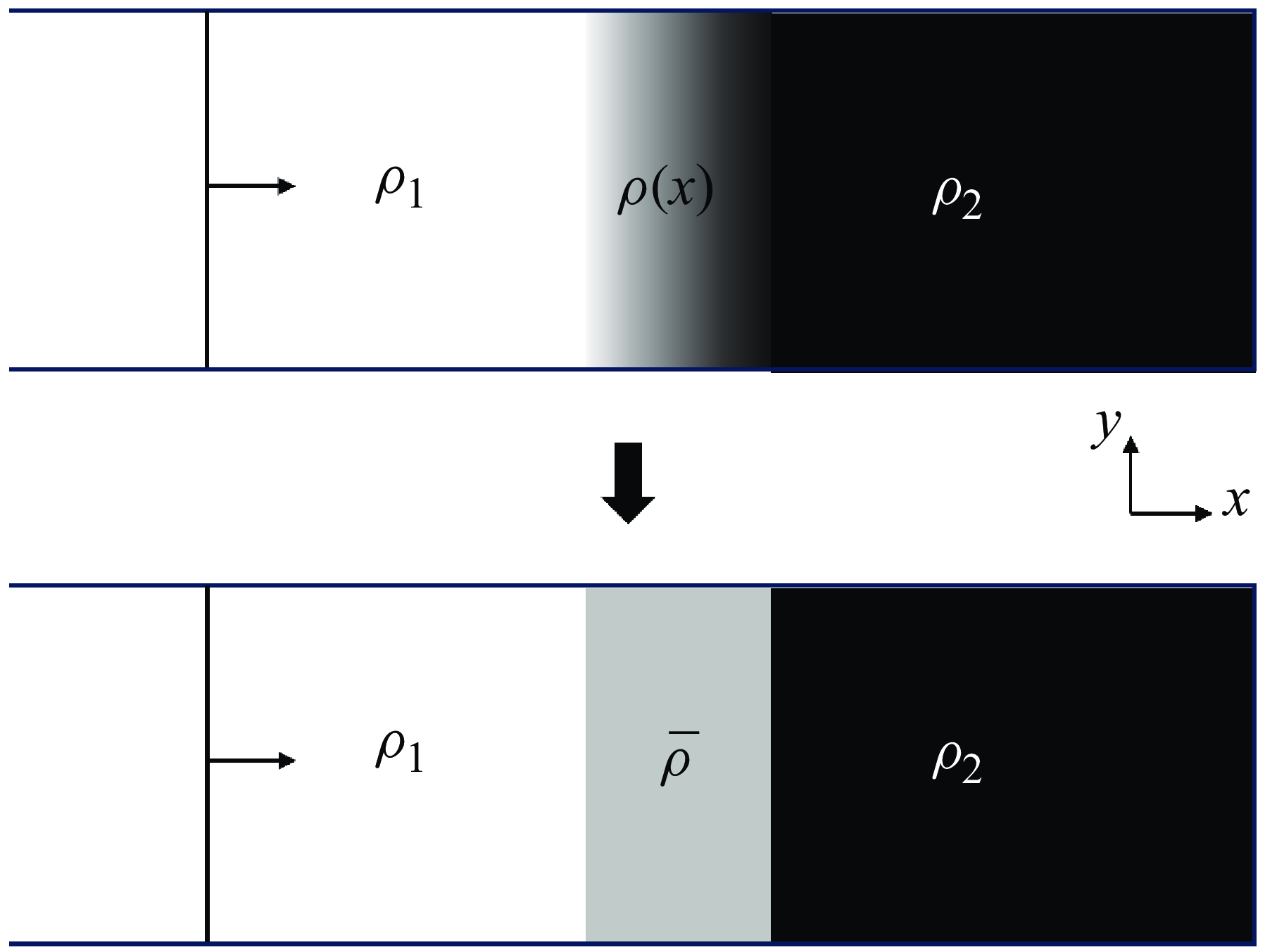
Schematic for simplifying a three-dimensional mixing area into a one-dimensional variable density area, where the depth of colour represents the magnitude of the density values.

To effectively model the stretching (compression) mechanism, it is essential to simplify the interaction between the shock wave and the light–heavy mixing region. As illustrated in figure 5, we treated the complex three-dimensional turbulent mixing zone as a one-dimensional region of variable density. This simplification was based on two key factors. First, the focus of the problem is the effect of the shock wave passing through the mixing zone on the overall mixing width, rather than the detailed changes in the three-dimensional structure. Consequently, adopting a one-dimensional representation is a practical and effective approach. This reduction enables a focused analysis of the fundamental physical mechanisms governing the interaction between the shock wave and the mixing zone, without being hindered by the intricacies of three-dimensional dynamics. Second, thorough mixing of the two media within the mixing zone is required to ensure that on a macroscopic scale, the physical properties of the turbulent mixing zone – such as volume fraction and density – can be adequately represented by a relatively smooth distribution through averaging. While this method neglects local fluctuations, it effectively captures the global characteristics of the mixing zone. The experimental results of Jourdan, Houas & Billiotte (Reference Jourdan, Houas and Billiotte1997) support this notion. They explored the evolution of the density distribution in the mixing zone as a shock wave propagating from
 $\text{CO}_2$
into gases such as helium, argon and krypton. The study focused on measuring the density evolution of
 $\text{CO}_2$
gas during fully developed turbulent states. The experimental results demonstrated close agreement between the observed data and the smooth curves derived from diffusion equations, thereby confirming uniform mixing across all cases. In conclusion, the assumption depicted in figure 5 remains valid when the mixing within the region is relatively uniform, and the research emphasis is placed on global rather than localized characteristics.
An
 $x{-}t$
diagram of a shock wave passing through light–heavy variable density regions, with thick solid lines representing the incident shock wave, thin solid lines representing the primary reflection wave, dashed lines representing the secondary reflection wave, and dotted lines representing the trajectory of fluid particles located on the leftmost side of the mixing zone.

To accurately characterize the physical process of a shock wave passing through a region of variable density, it is essential to first clarify the dynamics involved. The schematic in figure 6 shows the interaction of a shock wave with a region of variable density, where the light fluid
 $\rho _1$
is on the left, and the heavy fluid
 $\rho _{2}$
is on the right. Before entering the variable-density region OA, the incident shock wave propagates at a constant velocity, and the flow behind the wave remains uniform. Upon entering the variable-density region OA, the shock wave accelerates fluid particles on the left side of OA, rendering a velocity difference on both sides of the OA region. As the shock wave enters the variable-density region OA, the shock wave velocity changes in this region, and a once-reflected wave is generated simultaneously. When these once-reflected waves pass through the isentropic region between the incident shock wave and fluid particle path, they cause the fluid particle to decelerate and further generate twice-reflected waves. The twice-reflected wave travels in the same direction as the incident shock wave, and eventually exceeds the incident shock wave and subsequently interacts with it. These twice-reflected waves significantly affect the rate of velocity change when the shock wave passes through the variable-density region OA, and will also cause the incident shock wave to continue to change after passing through region OA. In the light–heavy variable-density region, the once-reflected wave is an isentropic compression wave, and the twice-reflected wave is a sparse wave. In the case of the heavy–light variable-density region, the properties of the once- and twice-reflected waves are reversed. In practical situations, higher-order reflection waves are generated; however, higher reflection waves are usually weaker, and their effects on shock waves and flow parameters in the mixing zone are relatively small.
During the process of the incident shock passing through the variable-density region OA, the fluid particles on the left side of the OA region are sequentially accelerated by the incident shock and decelerated by the once-reflected wave, resulting in a velocity difference on both sides of the OA region. The current issue is the change in the mixing width caused by the velocity difference on both sides of the variable-density region during the passage of the shock waves. In this problem, the propagation velocity of shock waves and the velocity difference on both sides of the mixing zone are no longer constant but depend on the density distribution of the mixing zone. We must establish a functional relationship
 $U_i(x)$
between the shock wave propagation velocity
 $U_i$
and spatial position
 $x$
, as well as a functional relationship
 $\Delta V(t)$
between the velocity difference
 $\Delta V$
on both sides of the mixing zone and the time
 $t$
based on the average density profile
 $\rho (x)$
in the mixing zone. Therefore, we refer to Chisnell’s early works (Chisnell Reference Chisnell1955). Chisnell considered the variable-density region as an infinite number of weak contact discontinuities, and derived the first-order relationship between shock intensity and density variation, as well as the first-order relationship between flow parameters and density variation, while ignoring twice-reflected and higher-order reflection waves. Whitham (Reference Whitham1958) further extended this method, and applied it to a large number of shock wave propagation problems in non-uniform media. Therefore, the result of this method is called the Chisnell–Whitham solution. Subsequently, Bird and others discussed the effectiveness of the Chisnell–Whitham method through numerical solutions using the characteristic line method (Bird Reference Bird1961). The results indicate that the effectiveness of this method depends on the intensity of the incident shock wave, the specific heat ratio of the gas, the shape of the density profile in the mixing zone, and the amplitude of the density changes. Given weak incident shock waves, high specific heat ratio gas combinations, and favourable density profile shapes, the Chisnell–Whitham solution yields high accuracy. If these conditions are not satisfied, then the method will cause certain errors. The introduction of twice-reflected and higher-order reflection waves significantly increases the theoretical complexity. Currently, no theoretical model fully replaces numerical simulations in providing precise predictions of shock wave and flow parameter variations within the mixing zone.
Given the complex physical phenomena involved in shock wave propagation through variable-density regions, as well as certain limitations of current theoretical analysis frameworks in describing such processes, it becomes impractical to directly obtain precise functional relationships such as
 $U_i(x)$
and
 $\Delta V(t)$
. As an alternative, we adopted a more practical strategy in this study, which involves solving the average propagation velocity
 $\overline {U}_i$
of the shock wave during the shock compression stage, and the average velocity difference
 $\overline {\Delta V}$
at both ends of the mixing zone. Based on this approach, this study introduces an innovative hypothesis; as shown in figure 7, by arithmetic averaging the density profile of the mixed zone, we simplified the variable-density region as a region with equivalent uniform density. The average density
 $\overline {\rho }$
is calculated using the equation
 \begin{equation} \overline {\rho }=\frac {\int _{x_1}^{x_2}\rho \left (x\right ){\rm d}x}{x_2-x_1}, \end{equation}
A schematic diagram of the variable-density region is assumed to be a uniform region, with the depth of colour representing the magnitude of the density values.

where
 $x_1$
and
 $x_2$
represent the positions at the two ends of the variable-density region. Simultaneously, the specific heat ratio in the uniformly dense region must also be averaged. Based on the assumption of linear superposition, the average specific heat ratio
 $\overline {\gamma }$
can be calculated as
 \begin{equation} \overline {\gamma }=\frac {\overline {c_p}}{\overline {c_v}}=\frac {\sum V_i c_{p, i}}{\sum V_i c_{v, i}}, \end{equation}
where
 $V_i$
represents volume fraction, and
 $c_p$
and
 $c_v$
represent the constant-pressure specific heat capacity and constant-volume specific heat capacity, respectively. The volume fraction
 $V_i$
exhibits the following intrinsic relationship with the mass fraction
 $Y_{i}$
(Youngs Reference Youngs2013):
 \begin{align} V_i= \frac{Y_{i}}{\left [Y_{i}+\left (1-Y_{i}\right )R\right ]}. \end{align}
Furthermore, if the density profile within the mixing zone and the densities of the fluids on both sides are known, then the relationship between the mass fractions of the two fluids in the mixing zone and the density profile can be established based on the principle of mass conservation, as
 \begin{align} \rho \left (x\right )= \frac{ 1}{\left[Y_{i} /\rho _{1}+\left (1-Y_{i}\right )/\rho _{2}\right]} \end{align}
Equation (3.15) was derived under the assumption that the two fluids are immiscible (Ruan et al. Reference Ruan, Zhang, Tian and Zhang2020; Zhang et al. Reference Zhang, Ni, Ruan and Xie2020b ,Reference Zhang, Ruan, Xie and Tian c ).
By solving the shock–interface interaction problem, the shock wave propagation velocity in the uniform-density region and the velocity at the left interface in the uniform-density region can be obtained. Specifically, this involves solving a coupled nonlinear system of equations governing the wave dynamics (Hurricane et al. Reference Hurricane and Miller1998). We assume that the propagation speed of the shock wave in the uniform-density region is the average velocity
 $\overline {U}_i$
of the shock wave, and that the velocity at the left interface of the uniform-density region is the average velocity difference
 $\overline {\Delta V}$
. Accordingly, the time of the interaction process between the shock waves and the variable-density regions can be approximated as
 \begin{equation} t=\frac {h^{-}}{\overline {U}_i}. \end{equation}
In summary, the contribution of the stretching (compression) mechanism to the variation in the mixing width in the light–heavy mixing zone shock compression problem can be approximated as
 \begin{equation} h_{III,S\left (C\right )}=\overline {\Delta V}\,\frac {h^{-}}{\overline {U}_i}. \end{equation}
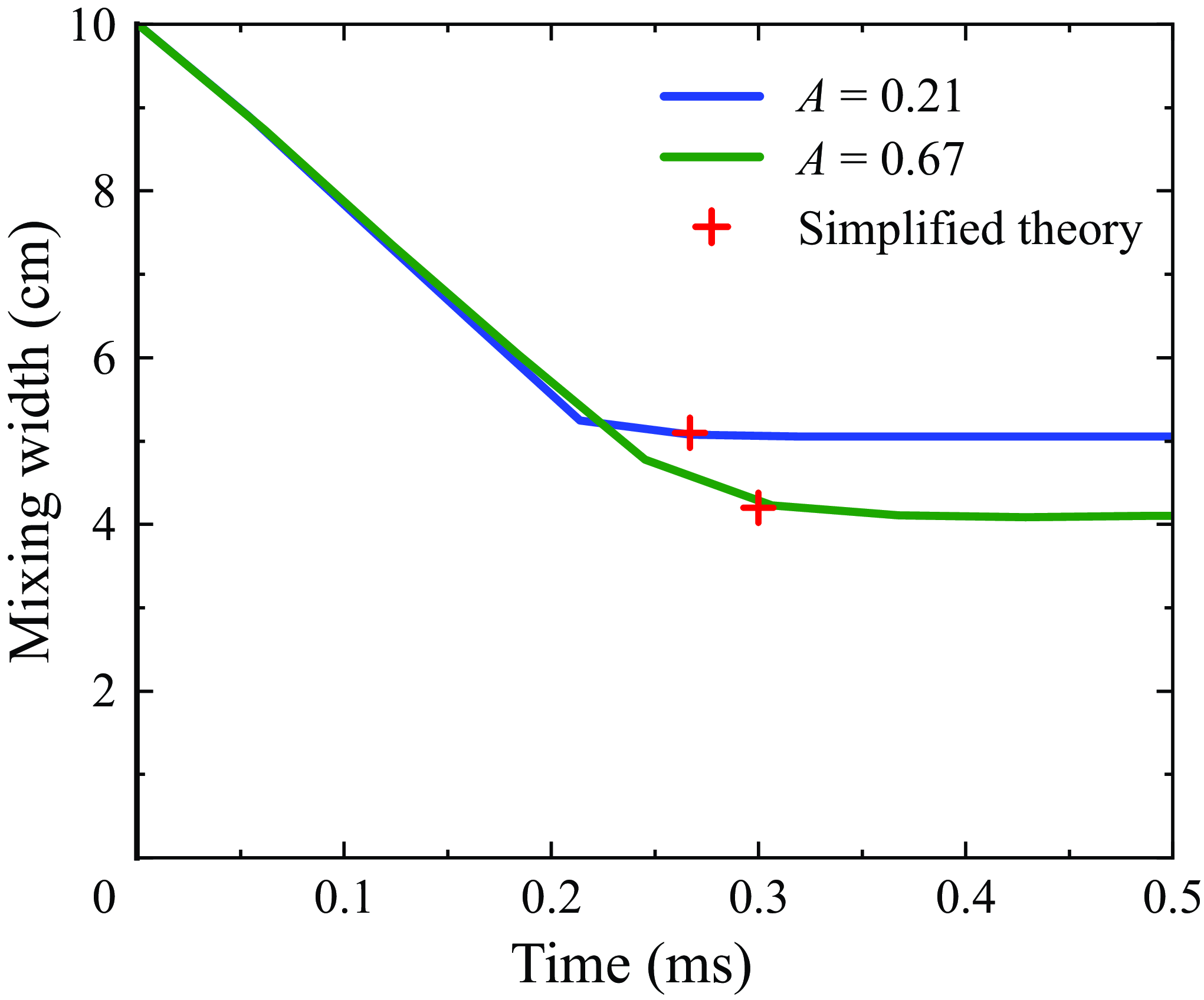
Comparison of simulation and simplified theory for mixed width compression of variable-density regions at different Mach numbers.

It should be noted that such simplified assumptions are inherently challenging to prove with absolute theoretical rigour. These assumptions are derived primarily from an intuitive understanding of the phenomena and practical considerations. Future research aims to develop more rigorous and accurate approximation theories to address these challenges. The focus of subsequent work will be to test the validity of this hypothesis through extensive numerical simulation experiments, thereby providing a simplified yet effective analytical framework for complex shock wave–variable-density mixing zone interactions without significantly compromising accuracy.
To investigate this problem, the one-dimensional Euler equations were solved to simulate the basic configuration of a one-dimensional shock tube flow. This numerical approach enabled the analysis of interactions between shock waves and regions of variable density. Experimental conditions, including the incident shock wave Mach number, the dimensionless density ratio of the fluids on both sides of the mixing zone, the initial width of the mixing zone, and the volume fraction profile of the light fluid (equivalent to the density profile), were varied systematically. This study compared the consistency and discrepancies between the predictions of the simplified theoretical model and the results of detailed numerical simulations. Specifically, figure 8 presents a comparison between the simplified theory and numerical simulations for incident shock wave Mach numbers 1.5 and 1.8. In this series of examples, the initial mixing zone width is
 $h^{-}=10\rm \ cm$
, with air and
 $\text{SF}_6$
on both sides of the mixing zone,
 $A=0.67$
, and the air volume fraction profile as a linear function. Figure 9 presents a comparison between the simplified theory and numerical simulations for air–
 $\text{CO}_2$
and air–
 $\text{SF}_6$
gas combinations, with Atwood numbers 0.21 and 0.67, respectively. In this series of examples, the Mach number of the incident shock wave is
 $M_i=1.5$
, the initial mixing zone width is
 $h^{-}=10\rm \ cm$
, and the air volume fraction profile is a linear function. Figure 10 presents a comparison between the simplified theory and numerical simulations for initial mixing zone widths
 $h^{-}=5$
and
 $10\rm \ cm$
. In this series of examples, the Mach number of the incident shock wave is
 $M_i=1.5$
, with air and
 $\text{SF}_6$
on both sides of the mixing zone, and the air volume fraction profile as a linear function. Figure 11 illustrates a similar comparison for cases where the volume fraction profile of the light fluid is modelled as either a linear function or an inverse proportional function. In this series of examples, the Mach number of the incident shock wave is
 $M_i=1.5$
, the fluids on both sides of the mixing zone are air and
 $\text{SF}_6$
, and the initial mixing zone width is
 $h^{-}=10\rm \ cm$
. The numerical simulation results are plotted in figures 8–11, indicating that the simplified theory can approximate the compression of the mixing width when a shock wave passes through a variable-density region.
Comparison of simulation and simplified theory for mixed width compression of variable-density regions under different Atwood numbers.

Comparison of simulation and simplified theory for compression of mixing width in variable-density regions under different initial mixing widths.

Comparison of simulation and simplified theory for compression of mixed width in variable-density regions under different light fluid volume fraction profiles.

To determine the contribution of the penetration mechanism to the change in the mixing width in formula (3.11), we employed the Sun et al. (Reference Sun, Song, Wang and Zhang2024) linear growth model (1.3) to characterize the effect as
 \begin{equation} h_{III,pen}=\left (C_M A \Delta u+\dot {h}_0^{-}\right )\frac {h^{-}}{\overline {U_i}}. \end{equation}
Based on (3.17) and (3.18), the evolution of the mixing width in the light–heavy multi-mode mixing zone shock compression problem can be calculated using the formula
 \begin{equation} \frac {h^{+}}{h^{-}}=1-\frac {\overline {\Delta V}}{\overline {U_i}}+\frac {C_MA \Delta u+\dot {h}_0^{-}}{\overline {U_i}}. \end{equation}
(IV) The last type of problem is the heavy–light multi-mode mixing zone shock compression problem. According to a previous analysis, the evolution of the mixing width in this problem was dominated by the stretching (compression) mechanism. The change in the mixing width
 $\Delta h$
can be expressed as
 \begin{equation} \Delta h=h_{IV,S\left (C\right )}\left (t\right ). \end{equation}
For the specific modelling method of
 $h_{IV,S (C )}$
, we have completely followed the simplified theoretical analysis framework used in problem (III); therefore, we will not elaborate on this further. The distinction between problems (III) and (IV) lies in the necessity of accounting for the contribution of the penetration mechanism to the mixing width in problem (III). Specifically, the evolution of the mixing width in the heavy–light multi-mode mixing zone during shock compression was determined using the equation
 \begin{equation} \frac {h^{+}}{h^{-}}=1-\frac {\overline {\Delta V}}{\overline {U_i}}. \end{equation}
4. Application of the shock compression model in reshock RM mixing
In the previous section, a mixing width prediction model was constructed to address four distinct shock compression scenarios: light–heavy interfaces, heavy–light interfaces, light–heavy mixing zones, and heavy–light mixing zones. To validate the accuracy of this model, it was compared against existing RM experimental and numerical simulation data.
Equation (3.6) was employed to predict specific changes in the mixing width of the light–heavy interface during shock compression. It is noteworthy that this equation shares the same mathematical form as (1.4), originally proposed by Richtmyer. This similarity arises from the fact that the equations are based on identical interface conditions, specifically the wavenumber and amplitude of the perturbation interface satisfying
 $ka_0\ll 1$
. Richtmyer’s formula has been validated extensively through RM instability experiments (Meshkov Reference Meshkov1969), demonstrating its robustness and accuracy, and it is therefore widely accepted in the field. Consequently, experimental validation of (3.6) is deemed unnecessary.
In examining the heavy–light interface shock compression problem, two phase-inversion phenomena were identified. Direct phase inversion occurs when the interface step velocity
 $\Delta u$
exceeds the shock wave velocity
 $U_i$
, resulting in physically unrealistic negative values when applying (1.4). This observation underscores the limitations of (1.4) in addressing shock compression at heavy–light interfaces: by analysing the physical processes behind both types of phase inversion, we introduced (3.10), designed to accurately describe the changes in mixing width in the heavy–light interface shock compression problem. To verify the accuracy of the model, we compared (3.10) with the experimental data of Holmes et al. (Reference Holmes1999), who investigated the evolution of single-mode RM instability under negative Atwood numbers using numerical simulations. They fixed the disturbance wavelength and amplitude to 100
 $\unicode{x03BC} m$
and 4
 $\unicode{x03BC} m$
, respectively, and reported numerical simulation results for incident shock Mach numbers 1.33, 5.6, 10.8 and 15.3. The numerical simulation data of the incident shock wave velocity and post-shock interface step velocity for the three cases are summarized in table 1. The data indicate that for Mach number 1.33, indirect phase inversion occurs. In contrast, a direct phase inversion was observed in the other three cases. In the dataset provided by Holmes et al. (Reference Holmes1999), time
 $t=0$
corresponds to the moment when the shock wave exits the perturbations region. Figure 12(a–d) present the numerical simulation results of the perturbations zone width compression compared with the predictions of (3.10). The results demonstrate that (3.10) accurately describes the compression behaviour of the perturbations zone width.
Numerical simulation data of Holmes et al. (Reference Holmes1999), with velocity in
 $\unicode{x03BC} {\textrm{m}}\ {\textrm{n}\,\textrm{s}}^{-1}$
.

Simulation and theoretical prediction comparison of shock compression problems at heavy–light interfaces under different shock Mach numbers. Numerical simulation data were obtained from a previous study (Holmes et al. Reference Holmes1999): (a) Mach 1.33, (b) Mach 5.6, (c) Mach 10.8, and (d) Mach 15.3. The Plots (a) and (b–d) correspond to the direct and indirect phase inversion of Formula (3.10), respectively.

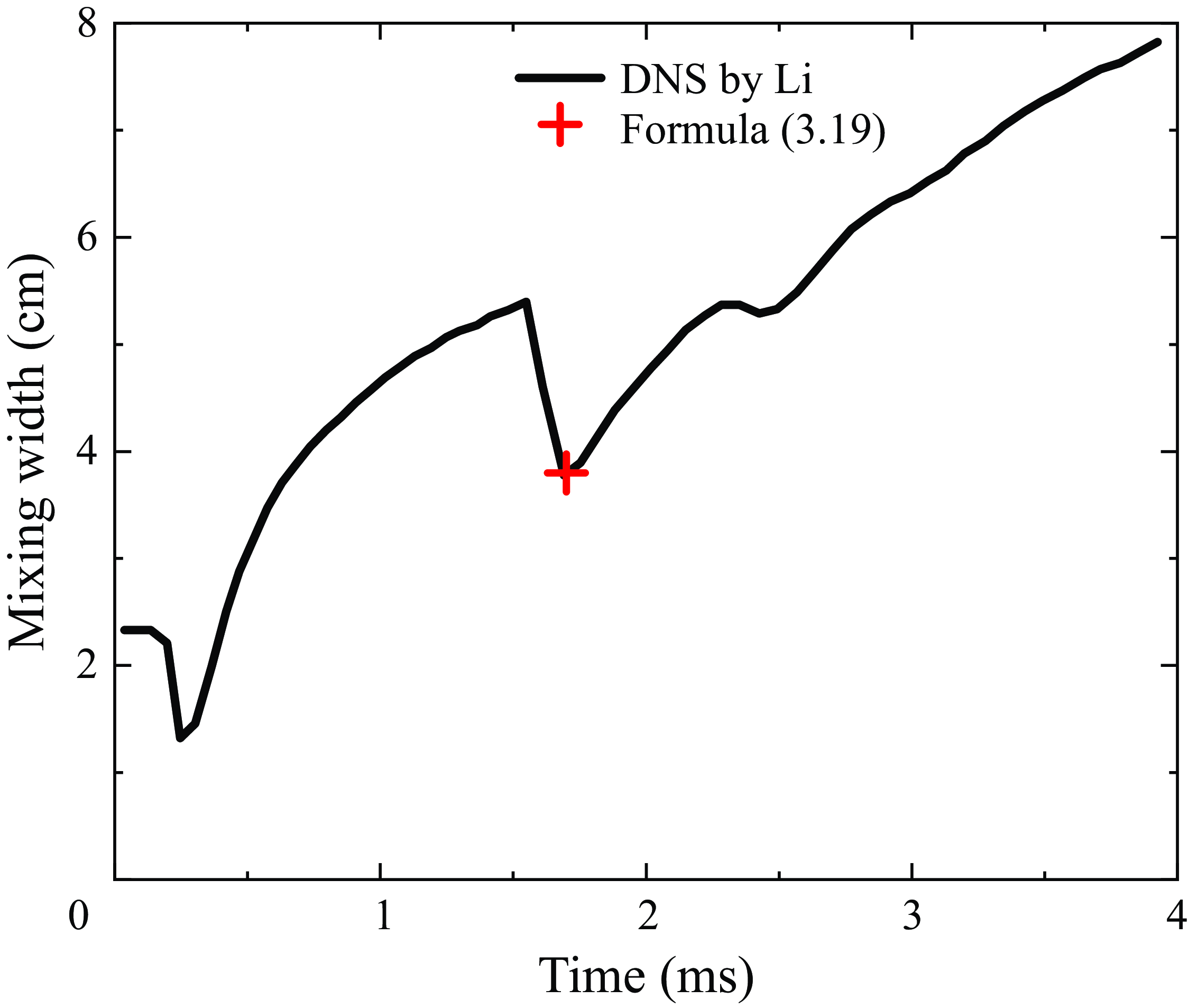
Equation (3.19) is used to predict changes in the mixing width for light–heavy mixing region shock compression problems, while (3.21) is applied to forecast variations in the mixing width for heavy–light mixing region shock compression problems. To assess the accuracy and applicability of these equations, comparisons were made with the DNS data provided by Li et al. (Reference Li, Tian, He and Zhang2021). These DNS data cover four different gas combinations: air–
 $\text{CO}_2$
, air–
 $\text{SF}_6$
,
 $\text{H}_2$
–air and
 $\text{SF}_6$
–air, documenting in detail the dynamic evolution process of the re-shock RM mixing width. Specifically, for the air–
 $\text{SF}_6$
combination, the heavy–light mixing region shock compression problem is considered during reshock, making it suitable for prediction using (3.21). For the combinations air–
 $\text{CO}_2$
,
 $\text{SF}_6$
–air and
 $\text{H}_2$
–air, the light–heavy mixing region shock compression problem is considered during reshock, for which (3.19) is applicable. Table 2 lists the initial gas parameters used in the numerical simulations conducted by Li et al. (Reference Li, Tian, He and Zhang2021); according to the simplified assumption proposed in the previous section, the calculation of the average velocity
 $\overline {U_i}$
and the average velocity difference
 $\overline {\Delta V}$
in (3.19) and (3.21) depends on the average density
 $\overline {\rho }$
and average specific heat ratio
 $\overline {\gamma }$
in the uniform-density region. Determining these average values requires knowledge of the volume fraction distribution within the mixing zone. A straightforward approach involves adopting a unified volume fraction profile for all RM mixing problems, which can be derived through theoretical analysis or numerical simulations. However, unlike RT mixing, for which a volume fraction profile independent of the density ratio has been established (Ruan et al. Reference Ruan, Zhang, Tian and Zhang2020; Zhang et al. Reference Zhang, Ni, Ruan and Xie2020b
,Reference Zhang, Ruan, Xie and Tian
c
), no theoretical solution for the volume fraction profile during the evolution of RM mixing currently exists. Due to the fundamental physical differences between RM and RT instabilities, the volume fraction profile for RM mixing is expected to depend on the density ratio of the two fluids. Consequently, using a uniform volume fraction profile across different RM problems may introduce errors. To minimize this error, the volume fraction profile of the mixing zone prior to reshocking was determined using one-dimensional shock tube simulations. These simulations were performed with the compressible fluid dynamics code
 $\text{CFD}^2$
developed by our research group for multi-medium flow problems, including RT and RM mixing. The code employs the finite difference method to solve the Reynolds-averaged Navier–Stokes equations, utilizing a K–L two-equation turbulence model. This turbulence model was specifically designed for mixing problems induced by interface instabilities, originating from the foundational work of Dimonte et al. (Reference Dimonte and Schneider2006). The K–L model employed in this study is an improved version developed by Xiao and others (Zhang et al. Reference Zhang, He, Xie, Xiao and Tian2020a
; Xiao, Zhang & Tian Reference Xiao, Zhang and Tian2021; Xie, Xiao & Zhang Reference Xie, Xiao and Zhang2024), and its adaptability to various mixing scenarios under different parameters has been validated thoroughly (Xiao, Zhang & Tian Reference Xiao, Zhang and Tian2020; Xie, Zhao & Zhang Reference Xie, Zhao and Zhang2023). Based on these profiles, we calculated the average density
 $\overline {\rho }$
and specific heat ratio
 $\overline {\gamma }$
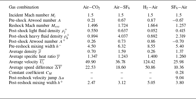
in the uniform-density region. Furthermore, all parameters involved in (3.19) and (3.21) are summarized in table 3. Subsequently, we compared the predicted results of (3.19) and (3.21) with the DNS data of Li et al. (Reference Li, Tian, He and Zhang2021) in detail, as shown in figures 13 and 14, respectively. The comparison revealed that the predictions from (3.19) and (3.21) were in strong agreement with the DNS data, thereby validating the accuracy of these equations.
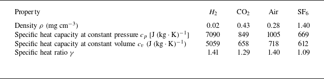
Properties of air,
 $\text{CO}_2$
,
 $\text{SF}_6$
and
 $\rm H_2$
.

Thermodynamic and kinetic parameters obtained from the theoretical calculations. The density unit is
 $\rm mg\ cm^{-3}$
, the velocity unit is
 $\rm cm\ ms^{-}{^1}$
, and the mixed width unit is
 $\rm cm$
.

5. Summary and discussion
The models presented in this study describe the evolution of the mixing width during the first shock and reshock phases in RM mixing problems. However, the evolution of the mixing width during the direct interaction between the shock wave and the interface or mixing zone has not been adequately addressed. In this work, the period during which the shock wave traverses the mixing zone is explicitly defined as the shock compression phase.
Comparison of numerical simulation and theoretical prediction of shock compression problems in heavy–light mixing zones. Numerical simulation data were obtained from a previous study (Li et al. Reference Li, Tian, He and Zhang2021). The initial interface was (a) air–
 $\text{CO}_2$
, (b) air–
 $\text{SF}_6$
, (c)
 $\text{H}_2$
–air.

Numerical simulation and theoretical prediction comparison of shock compression problems in light–heavy mixing zones. Numerical simulation data were obtained from a previous study (Li et al. Reference Li, Tian, He and Zhang2021). The initial interface was
 $\text{SF}_6$
–air.

Initial analysis of the direct numerical simulation data from Li et al. (Reference Li, Tian, He and Zhang2021) revealed that the mechanisms driving the evolution of the mixing width during the shock compression phase are relatively complex. These mechanisms can, however, be classified into two distinct types based on the direction of the shock impact. A detailed analysis of the shock interface compression process led to a qualitative classification of the shock compression problem into two primary categories. For light–heavy shock compression problems, the evolution of the mixing width is governed by the combined effects of the stretching (compression) mechanism and the penetration mechanism. In contrast, for heavy–light shock compression problems, two types of phase inversion phenomena occur, resulting in evolution predominantly driven by vorticity, with minimal impact on the overall mixing width. Consequently, heavy–light problems are primarily controlled by the stretching (compression) mechanism, while the penetration mechanism can be largely disregarded.
In RM mixing problems, the first shock and reshock phases involve the compression of the interface and the mixing zone, respectively. Based on this understanding, shock compression problems were further categorized into four distinct types:
-
(i) light–heavy interface shock compression
-
(ii) heavy–light interface shock compression
-
(iii) light–heavy mixing zone shock compression
-
(iv) heavy–light mixing zone shock compression.
By independently modelling the stretching (compression) and penetration mechanisms, predictive models were developed for each of the four types of shock compression problems. For single-mode/multi-mode interface-related problems (types I and II), (3.6) and (3.10) were derived. These equations remain valid under the condition that the interface perturbations satisfy linearity. Equation (3.10) further elucidates both direct and indirect phase inversions, which necessitates resolving the shock–interface interaction problem to capture these two types of phase inversions. For nonlinear multi-mode mixing zone-related problems (types III and IV), the modelling process was simplified by approximating the mixing zone as a uniform-density region. This approach led to the derivation of (3.19) and (3.21), which demonstrate strong agreement with numerical simulation data.
While Richtmyer originally solved the compression of linear single-mode perturbations, we argue that his solution applies exclusively to scenarios where the shock propagates from a light to a heavy fluid. In this work, we clarify the distinction between the shock propagating from a heavy to a light fluid and the former case, and have generalized the model to linear multi-mode perturbations. We emphasize that although (3.6) and (3.10) can predict the compression of linear single-mode/multi-mode perturbations, they may fail to predict the nonlinear evolution of single-mode/multi-mode perturbations when the precondition
 $ka \ll 1$
in the single-mode problem, or
 $k_ia_i \ll 1$
for all
 $i$
in the multi-mode problem, is not satisfied. This limitation arises because the initial interface evolves immediately into a nonlinear regime, with the appearance of complex bubble and spike structures. The contribution of the stretching (compression) effect to the compression of disturbances is challenging to quantify, making this a compelling topic for future investigation. For nonlinear multi-mode mixing zone problems, the actual mixing zone was approximated as a uniform-density region. A simplified theoretical model was proposed to describe the traversal of the shock through this region. While this model was validated against numerical simulations, it remains a theoretical approximation, with further refinement needed to fully capture the underlying physical processes. Future studies focused on developing detailed theoretical models of shock interactions with the mixing zone would undoubtedly enhance the findings of this work and contribute to a deeper understanding of RM mixing dynamics.
Beyond the shock compression phase modelling investigated in this work, another unresolved issue in reshocked RM mixing lies in the duration of the linear growth phase of the mixing zone following reshock, specifically the modelling of
 $t^{*}$
in (1.2). Mikaelian initially formulated an expression for
 $t^{*}$
using the pre-reshock mixing width
 $h^{-}$
and the post-reshock mixing zone step velocity
 $\Delta u$
, treating the dimensionless coefficient in the expression as a constant. However, we argue that the modelling of
 $t^{*}$
can be refined with greater physical nuance. The selection of the length scale in the expression – whether the pre-reshock mixing width, post-reshock mixing width, or a combination thereof – warrants detailed scrutiny. First, the chosen length scale should reflect the physical mechanisms governing the linear growth phase after reshock, as
 $t^{*}$
inherently characterizes the decay time scale of this regime. Second, the selected scale must ensure that the dimensionless coefficient in the
 $t^{*}$
expression carries a well-defined physical interpretation. This coefficient could either remain universal or depend on parameters such as the Atwood number and Mach number. A judicious choice of length scale may unify the interpretation of this coefficient across a class of problems. Critically, the final
 $t^{*}$
formulation must align with existing experimental data to validate the appropriateness of the chosen length scale. Addressing this challenge represents a pivotal direction for future research.
Acknowledgements.
The authors acknowledge financial support provided by the National Natural Science Foundation of China (grant no. 12222203) and the Foundation of the National Key Laboratory of Computational Physics (grant no. 6142A05240201).
Declaration of interests.
The authors report no conflict of interest.