1. Introduction
We investigate the role that economic instruments can play in supporting developing countries to preserve biodiversity while simultaneously aiming at economic sustainability. Our study incorporates scientific ecological findings on the role of pollination services into an economic analysis of agroforestry in coffee production. Coffee is an interesting case as it ranks among the world's five most valuable export commodities (USD 7 billion in 2004) and coffee production employs about 25 million people (FAOSTAT, 2005; Ricketts et al., Reference Ricketts, Daily, Ehrlich and Michener2004). Most coffee producers live in poverty and manage agro-ecosystems in some of the world's most culturally and biologically diverse regions in Latin American, Asian, and African countries (Bacon, Reference Bacon2005). Despite increasing evidence that the abundance and diversity of bees may augment pollination and boost coffee crop yields (Roubik, Reference Roubik2002; Klein et al., Reference Klein, Steffan-Dewenter and Tscharntke2003a,Reference Klein, Steffan-Dewenter and Tscharntkeb,Reference Klein, Steffan-Dewenter and Tscharntkec), shade trees on plantations and forest strips near coffee farms are removed for the sake of greater short-term efficiency. The resulting loss of pollinator habitats is a considerable environmental problem worldwide (Kremen and Ricketts, Reference Kremen and Ricketts2000). Moreover, fluctuation in international coffee prices due to, among other things, occasional overproduction worsens the situation of impoverished farmers and may prompt the destruction of the remaining forest strips.
Some recent studies have drawn attention to the economic value of pollination services that are reflected as agroforestry benefits in coffee production systems (see, e.g., Ricketts et al., Reference Ricketts, Daily, Ehrlich and Michener2004). Gobbi (Reference Gobbi2000) found that investment in biodiversity-friendly certification criteria is financially viable for coffee farms, while Benítez et al. (Reference Benítez, Kuosmanen, Olschewski and van Kooten2006), Ninan and Sathyaplan (Reference Ninan and Sathyaplan2005), and Olschewski et al. (Reference Olschewski, Tscharntke, Benítez, Schwarze and Klein2006) note that the high opportunity costs of land managed by ecological principles, in terms of lost benefits of intensely cultivated coffee or alternative crops, precipitates biodiversity degradation. An overall conclusion from the studies focusing on the value of pollination services is that policy measures such as trade-related standards, premiums, forms of tax relief, or dedicated government institutions are necessary for the adoption of biodiversity-friendly growing practices (see also Damodaran, Reference Damodaran2002; Bacon, Reference Bacon2005; Perfecto et al., Reference Perfecto, Vandermeer, Mas and Pinto2005).
Another strand of related literature has considered alternative policy instruments for protecting endangered natural ecosystems. For example, Ferraro and Simpson (Reference Ferraro and Simpson2002) and Ferraro et al. (Reference Ferraro, Uchida and Conrad2005) found that direct methods such as conservation payments are more cost-efficient than indirect methods such as output and investment subsidies when policy programs aim to achieve large increments in biodiversity conservation areas. Interestingly, the empirical results of these case studies on apiculture in Madagascar may in fact hint at a possible reason for the popularity of indirect methods compared to direct ones: income in the recipient low-income nations rises considerably with even a small increase in the protection of rain forests through indirect means. Increased income is often the most important goal in many projects motivated by long-term sustainability and eradication of poverty (see, e.g., Ferraro and Kiss, Reference Ferraro and Kiss2002; Swart, Reference Swart2003). Eradication of poverty has not been considered explicitly in biodiversity studies. We investigate the performance of alternative economic instruments and study whether direct methods are still better given two different simultaneous goals, protection of biodiversity, and sustainable income.
We augment previous policy analyses by modeling explicitly the ecosystem services provided by pollinators. To gain insights into land allocation processes, the choice between environmentally detrimental and sustainable farming technology is determined in our model by the relative profits of the technologies (cf., e.g., Bulte and Horan, Reference Bulte and Horan2003). We focus on the technologies for shade- and sun-grown coffee. In particular, we study what drives technology choices when the economic optimization is carried out by several small farmers or a sole owner. We investigate the conditions under which farmers specialize in either shade- or sun-grown coffee or whether both practices coexist.
Finally, we investigate the impacts of three alternative policy tools on the choice of shade or sun coffee production: (1) price premiums, (2) conservation payments, and (3) minimum wages. All of these instruments can be used for reducing environmental degradation but they work differently. Fair trade/eco-labeling is an example of a market-based conservation strategy whereby consumers pay a premium price for coffee produced on certified farms committed to the preservation of biodiversity and/or fair working conditions (see, e.g., Perfecto et al., Reference Perfecto, Vandermeer, Mas and Pinto2005; Swallow and Sedjo, Reference Swallow and Sedjo2000; Sedjo and Swallow, Reference Sedjo and Swallow2002). Conservation payments are an example of targeted aid, which is typically used for establishing protection areas (see, e.g., Ferraro and Simpson, Reference Ferraro and Simpson2002). A minimum wage represents a policy instrument designed for reducing inequality and preventing rural outmigration in developing countries (Lustig and McLeod, Reference Lustig, McLeod, Edwards and Lustig1997; Gindling and Terrell, Reference Gindling and Terrell2005; Lall et al., Reference Lall, Selod and Shalizi2006). We study whether instruments aimed primarily at providing sustainable income (such as minimum wages) and, on the other hand, at protecting biodiversity (conservation payments) lead to conflicting outcomes when the input use intensity or production cost structure of alternative technologies differs. We compare these two specialized instruments to a third instrument in between the two, i.e. price premiums based on fair trade and eco-labels, which arguably target both economic and environmental aspects of sustainability (Rice and McLean, Reference Rice and McLean1999).
We calibrate an empirical model to describe the choice of technology at the level of a representative local community in Costa Rica, where coffee production has been one of the most important factors in the economic development (Agne, Reference Agne2000). Furthermore, deforestation has traditionally been an important environmental problem in northern Latin America. Our empirical analysis facilitates a characterization of the alternative equilibria in land use and illustrates the magnitude of the ecological and economic impacts of the alternative policy measures.
Our study contributes to the previous literature by approaching the valuation of pollination services from a new angle. We recognize that maintaining environmentally sustainable farming practices requires a considerable allocation of resources to this technology to guarantee its existence, and the opportunity costs of conservation may become very high. Furthermore, trade-offs between the conservation of biodiversity and sustainable income should be taken into account when designing conservation policies. Our results indicate that a policy instrument explicitly designed for promoting economic (social) sustainability may conflict with the goals of conserving biodiversity and vice versa.
The rest of the paper is organized as follows. In section 2, we discuss the basic background concepts of this paper, namely coffee production and its relation to pollination and biodiversity. In section 3, an analytic model is presented and in section 4, it is applied to a specific case. Finally, section 5 provides conclusions.
2. Coffee production, pollination, and biodiversity
In this section, we review the basic characteristics of coffee production, the importance of insect pollination to it, and the characteristics of the two production technologies discussed in this study. Rather than attempting to provide a comprehensive treatment of these issues, we concentrate on aspects that are relevant from the point of view of our model and application. The main consideration is that coffee can, in our framework, be produced using two alternative methods and that the implications of the production methods for biodiversity and economic profitability differ crucially from each other.
2.1. Coffee markets, production, and pollination
The demand for coffee has been fairly stable in recent years. However, the demand for certified fair trade and organic gourmet coffee has been growing fast, especially in the United States and the European Union, although their market share is still very small (Bacon, Reference Bacon2005; Raynolds et al., Reference Raynolds, Murray and Taylor2004). On the other hand, supply fluctuates substantially, primarily due to weather conditions. This variation is exacerbated by the fact that coffee takes about three years from planting to harvest (one and a half years for hybrid variants), and thus the harvest area cannot be quickly altered to maintain a stable supply. In addition, coffee has a biannual production cycle, which further limits the possibility to adjust production to the market situation (Agne, Reference Agne2000; Dicum and Luttinger, Reference Dicum and Luttinger1999). As a result, the average price of coffee has fluctuated quite significantly.
Coffee production can be roughly analyzed in terms of two main methods.Footnote 1 The traditional method (‘shade coffee’) is to grow coffee plants among shade trees, which may produce alternative products of economic value (e.g., fruit and medicine) (Bray and Merino-Pérez, Reference Bray and Merino-Pérez2002). This method involves relatively fewer coffee plants per hectare, relatively slower growth, and a smaller yield per plant, and a lesser need for commercial inputs. On the other hand, the method has positive impacts on biodiversity (Méndez et al., Reference Méndez, Gliessman and Gilbert2007) and the soil and provides for a relatively longer plant life span. The second common method originated with the Green Revolution and involves growing coffee in the open without shade (‘sun coffee’). These plantations are de facto monocultures with intense production. The method allows more coffee plants per hectare and produces a relatively quicker and higher yield per plant. However, it has negative impacts on biodiversity and soil, shortens plant life span, and imposes reliance on a single crop (coffee).
About two-thirds of the world's crop species include cultivars that require animal pollination and approximately one-third of food consumption in tropical countries originates from plants that are insect pollinated (Kremen et al., Reference Kremen, Williams and Thorp2002; Rickets et al., Reference Ricketts, Daily, Ehrlich and Michener2004). Two main coffee variants are used in production. The highland variety, Coffea arabica, is grown mainly in South and Central America and the lowland variety, Coffea canephora var. robusta, mainly in West Africa and Southeast Asia, although this geographical division has begun to disintegrate (Dicum and Luttinger, Reference Dicum and Luttinger1999). C. arabica is self-pollinating, but it has been shown that cross-pollination by insects may increase the fruit set.Footnote 2 C. canephora is self-sterile and predominantly wind-pollinated but has been shown to produce higher fruit sets when pollinated by both wind and insects. In addition, cross-pollination is likely to lead to larger and more robust fruit, increasing both the quality and quantity of the crop (Klein et al., Reference Klein, Steffan-Dewenter and Tscharntke2003a,Reference Klein, Steffan-Dewenter and Tscharntkeb,Reference Klein, Steffan-Dewenter and Tscharntkec; Ricketts et al., Reference Ricketts, Daily, Ehrlich and Michener2004; Roubik, Reference Roubik2002).
It has recently been shown that both the diversity and abundance of bees are important for pollination. Biological diversity provides greater and more predictable pollination services, which in turn increase the fruit set (and thus the yield) of coffee plants. Bee diversity and abundance decrease with the distance from the nearest forest, whereby the fruit set of coffee plants pollinated on open ground is inversely correlated with that distance. In order to maintain the pollination services provided to coffee plants by wild bee populations, the forest habitat of the bees must be conserved (Klein et al., Reference Klein, Steffan-Dewenter and Tscharntke2003b,Reference Klein, Steffan-Dewenter and Tscharntkec; Kremen et al., Reference Kremen, Williams and Thorp2002; Ricketts et al., Reference Ricketts, Daily, Ehrlich and Michener2004; Steffan-Dewenter and Tscharntke, Reference Steffan-Dewenter and Tscharntke1999).
2.2. Implications for modeling
In our specification, sun coffee is intensively produced and generally hand pollinated, and thus whether or not there are pollinating insects nearby is of little relevance. In contrast, insect pollination is important for shade coffee production. In fact, any two crops of which one is insect pollinated and the other is not could be substituted for shade and sun coffee. In a sense, we are comparing shade coffee production to the most profitable alternative (represented here by sun coffee); considering more than one alternative would not benefit our analysis.
Accordingly, in our model the shade coffee system includes a compulsory forest strip serving as a pollinator habitat. This is in line with certification programs, which set standards requiring that a minimum percentage of the farm area facilitate biodiversity (Rice and McLean, Reference Rice and McLean1999). Thus, whereas the per hectare yield of sun coffee is assumed to be constant, the yield of shade coffee depends on the distance between the plantation and the nearest forest. We assume that the decisive factor in pollination is the distance from the nearest forest, not the existence of shade trees as such. Moreover, the size of the forest depends on the area that is allocated to shade coffee; a portion of the land allocated to shade coffee production is covered by forest.
In the present study, the forest is assumed to be located at the edges of the shade coffee area. This is in contrast to the approach of Olschewski et al. (Reference Olschewski, Tscharntke, Benítez, Schwarze and Klein2006), who assume that the cultivated region surrounds the forest. In practice, depending on the landscape the stretches of forest could form a more complex pattern. In this paper, the location and size of the forest are not choice variables for farmers. The assumption that the forest surrounds the shade coffee region is a simplification that aims to internalize the externality of forest strips having a positive impact on the production of shade coffee. Situating forest strips in a more sophisticated pattern could produce more efficient pollination and higher yields. However, considering the optimal design of forest patches would lead to a complex spatial optimization problem that is beyond the scope of this paper. Instead, our main interest is in a comparison of alternative production technologies, and we investigate the diverse impacts on the production of shade coffee resulting from an internalization of a positive externality of forests strips. The declining average productivity with respect to distance from the forest strips is the key feature here. For the forest to be of any relevance as a pollinator habitat we need to model a forest area that is perhaps larger than the ones currently had in some instances.
Certain other aspects of our empirical model require comment. First, price volatility is not accounted for in our deterministic analysis. However, as long as both prices (sun and shade coffee) move together, their volatility has no effect on the choice of production technology. Moreover, coffee plants are long lived and it is therefore reasonable to assume that farmers make decisions according to long-run averages rather than adjust their technology choices rapidly according to market conditions. Second, shade coffee technology attracts a price premium on the international market, thus giving a higher producer price. It is worth noting that in practice the mere fact that a farm produces shade coffee does not provide any price premium. It is only when the production has been certified through some scheme that this benefit materializes. Although fair trade and eco-certification are different, the overall aim of both of these schemes is to promote ‘sustainable’ coffee production (see Kilian et al., Reference Kilian, Jones, Pratt and Villalobos2006). We assume an arbitrary certification scheme for shade coffee and that any costs of certification are already taken into account in the production costs. We also study how a standard (such as size of forest area) set in a certification program affects the ranking of policy instruments.
We are dealing with prices as they materialize for the producer, and hence the price premium refers to the premium that the producer receives. We analyze the problem in a partial equilibrium context and thus ignore the potential impacts on intermediaries or any other parties concerned. Third, shade coffee production involves a higher production cost per hectare due to the need for more labor in production. Coffee production thus involves both economically and environmentally important dimensions. Accordingly, the two production technologies analyzed in this study have been chosen as differing in (i) yield per hectare; (ii) producer price per kilogram; (iii) production costs per kilogram; (iv) production costs per hectare; and (v) dependence on forests and pollination.
3. The model
We first derive the profit functions of sun coffee and shade coffee technologies. We then investigate two different farm structures: sole ownership and small-scale farms. Under sole ownership there is a single decision maker, who chooses an optimal land allocation between sun coffee and shade coffee. In the other setting, several small-scale farmers in the community make decisions between the two technologies. We do not consider how the small farms are actually situated and assume that the shape of the shade coffee cultivation region is independent of individual farmers’ actions. This makes it possible to formulate a static equilibrium model that need not take into account the process that would actually take place when farmers make their technology choices. Our focus is on describing the economic outcome of that process.
We let A denote the total area of land that is allocated to coffee production. The two technologies for coffee production, sun and shade coffee, are indexed by 1 and 2, respectively. The variable μ denotes the proportion of the area that is allocated to shade coffee production. The proportion that is allocated for sun coffee is then (1−μ).
3.1. Profit functions
We assume that the yield of sun coffee depends only on the area which is allocated to its production. Hence, the effect of pollination on the yield is assumed to be negligible, which is in fact the case since, as mentioned earlier, the plants are pollinated manually. The yield is then simply (1−μ)Y 1A, where Y 1 is the yield per hectare. We divide the costs of producing coffee into two categories: costs that depend on the yield, e.g. harvesting and transportation costs (c 1), and costs that depend on the area under production, e.g. pest control and fertilization costs (e 1). Labor costs account for most of the area-dependent costs. When the per unit producer price of sun coffee is p 1, the profits are

In the case of shade coffee, we assume that the yield depends on the distance of the coffee plant from the border of the pollinator source (forest), as shown by Klein et al. (Reference Klein, Steffan-Dewenter and Tscharntke2003c). We assume that the shade coffee region is surrounded by a forest strip that has a fixed width, δ0. In other words, for any given area of shade coffee production, the forest either covers a strip of width δ0 or, if the area is very small, the forest covers the whole area. The yield declines with distance from the forest, but there is a certain minimum y min below which the yield cannot fall. We also assume that the plot that is allocated to shade coffee production has the same shape as the total area. More specifically, the shape of the region in which shade coffee is produced remains unchanged, but its size may vary as the allocation of area to shade coffee production changes. We let Y 2(μ) denote the shade coffee yield when portion μ of the total area is allocated to shade coffee. The full details of the yield function are presented in the Appendix A.1 (Appendix at http://journals.cambridge.org/EDE).
The total profit of shade coffee is obtained by subtracting the area-dependent costs from the net returns of yield and adding the potential income from the forest strip C(μ)

where p 2 is the shade coffee producer price, c 2 is the yield-proportional cost factor, e 2 is the area-proportional cost factor, and p 3 is the per hectare value obtained from the forest strip; for instance, a conservation fee. In section 4.1, we shall study p 3 as a policy instrument; initially it is set to zero. Note that we do not explicitly allow the farmers to allocate their land to forest; rather, the forest area always depends on the area allocated to shade coffee. This is to highlight the importance of analyzing the choice of technology (sustainable/unsustainable) when sustainable technology is in practice determined by the requirements of a certification program. However, as long as p 3 is reasonably low it plays the role of a conservation payment rather than of a subsidy paid to shade coffee producers. Since the forest strip does not cause any costs, we subtract C(μ) from the total area in the second term of the sum in (1). We have excluded the possible extra profits from the products of shade trees in the profit function π2. These products may include medicines, foods, construction materials, and forage (Moguel and Toledo, Reference Moguel and Toledo1999).Footnote 3
In our empirical application, the area-dependent costs e 1 and e 2 are decomposed into labor costs and other costs. More specifically, the costs are assumed to be of the form

where i∈{1, 2} and li is the amount of labor required for using technology i in person-months per hectare, w the wage in dollars per month, and zi area-dependent costs other than labor costs.
3.2. Equilibria and the joint profits maximum
We study two different farm structures: sole owner and small-scale farms. In the former setting, the land allocation decision between shade and sun coffee is made by maximizing the joint profits of the two technologies, i.e. π1(μ)+π2(μ). In the latter setting, we assume that there are a large number of small-scale farmers who decide whether to belong to the community of sun or shade coffee farmers and that these farmers make their decisions without any coordination. Our model of land allocation is static. Hence, we shall not consider how the equilibria and optima are reached or how a farm's forest strips are formed in the process of reaching the solution.
A sole owner allocates land to either of the two technologies by satisfying the first-order optimality condition dπ1(μ)/dμ+dπ2(μ)/dμ = 0, which can be written as

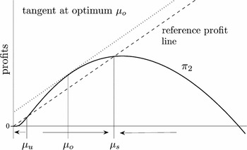
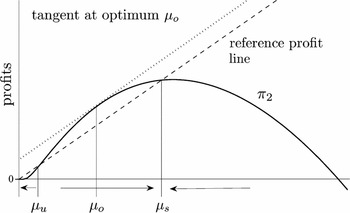
The right-hand side of (3) is the marginal profit from sun coffee, i.e. the marginal increase in profits for an increase in (1−μ). Condition (3) says that the marginal profits of the two technologies are equal in the optimum. Geometrically, the optimum is at the point where π2 has a tangential line with slope A[(p 1−c 1)Y 1−e 1]. This is illustrated in figure 1, where the dotted line is the tangent of π2 at the joint profits maximum.
Illustration of π2, the optimality and equilibrium conditions
In the small-scale farm setting there are many farmers, whereby each farmer's marginal contribution to the profitability of the technology is negligible. The total profits from the technology chosen are shared in proportion to farm size. Thus, for a farmer whose land covers an area Δ of the community, the profits from sun coffee production will be Δ×π1(μ)/[(1−μ)A] and from shade coffee production Δ×π2(μ)/(μA). This means that the farmers’ land allocation choices between the two technologies depend on the profitability of the technologies. Notice that an individual farmer has to choose between the technologies and cannot allocate land to both sun and shade coffee. In practice, this means that the costs of having two production methods are prohibitively large for a small producer. Hence, an individual farmer faces a problem of technology choice rather than of land allocation.
By assuming that farmers make their choice according to the profitability of the technologies, we avoid considering the location of the plot of an individual farmer. Profitability as the choice criterion has two main interpretations. First, farmers do not receive profits from individual plots but instead form a community that shares the profits equally. Second, when making their choices, farmers may be uncertain or unaware of the actual profits they receive; profitabilities represent their expectation regarding profits.Footnote 4 We emphasize that farmers or the communities do not coordinate their technology choice decisions and these decisions are definitive.
Since farmers choose their production technology on the basis of profitability, an equilibrium is reached when the profitabilities are the same. Namely, if one of the technologies is more profitable, then at least some of the farmers will be willing to change technologies. Profitability is measured as profits per hectare and the profitability factors are θ1 = π1/[(1−μ)A]=(p 1−c 1)Y 1−e 1 and θ2 = π2/(μA). At equilibrium, none of the farmers has an incentive to change from one technology to another, which means that θ2 = θ1. This condition can be written as

and we shall refer to the line π = μA[(p 1−c 1)Y 1−e 1], μ∈[0, 1], as the reference profit line, because it gives the profit from sun coffee production if a proportion μ of land area is allocated to sun coffee instead of shade coffee (see figure 1). Note that the slope of the reference profit line is the same as the right-hand side of (3). The difference between the two farm structures is that a sole owner allocates land according to marginal profit whereas small-scale farmers choose the technology according to average profitability.
Assuming that the equilibrium μ* is on the interval (0, 1), we observe that the equilibrium profits π1(μ*)+π2(μ*) are equal to the profits obtained when the whole area is allocated to sun coffee. This follows from the fact that shade coffee has the same profitability as sun coffee in equilibrium. Consequently, the total equilibrium profits are unaffected by the price of shade coffee, p 2, and its production costs, c 2 and e 2, as long as the equilibrium is on the interval (0, 1). Similarly, introducing a conservation fee, p 3, alters only the equilibrium allocation but not the total profits.
Let us now focus on the properties of the profit function of shade coffee production, π2. For a small enough μ, the corresponding profit π2(μ) is zero, because the whole area allocated to shade coffee is covered by the forest strip; recall the assumption on the fixed width of the forest strip. The profit π2 starts to increase after the forest strip has reached its minimum width, δ0. Depending on the parameter values, the marginal profit decreases for a large enough μ. The decreasing marginal profits follow from the fact that the proportion of the area in which the yield is y min increases and the proportion of the area in which the pollination is effective decreases. As μ increases, a larger proportion of the yield comes from the area which is far from the forest. In particular, a larger proportion of the yield is produced in the area in which the yield per plant is y min. However, when shade coffee production is extremely profitable, it may happen that the marginal profit increases along the entire interval (0, 1) after the point at which π2 becomes positive. In the other extreme case when shade coffee has low profitability, there is a point after which the profit decreases. An example of such a profit function is provided in figure 1, where the reference profit line is represented by a dashed line.
If the location of forest patches were designed optimally, it might be possible to reduce the region inside of which the yield is y min. For example, this could be done by locating forests in a complex mosaic throughout the region. Recall, however, that in our model farmers are not free to locate the forests as they wish. Moreover, in the small-scale farmer setting the farmers’ land allocation choices are uncoordinated. Optimal location of forests would, however, require coordination of land use. In the case of a sole owner, the optimal design of forest patches would make sense. However, we rule out this possibility, as we then could not disentangle the impact of distance from forest strips in the two alternative farm structure settings.
As seen in figure 1, π2 crosses the reference profit line twice, and there are two equilibria, μu and μs. On the interval (μu, μs), the profit function π2 is above the reference profit line, which means that the profitability of shade coffee is greater than the profitability of sun coffee, i.e. θ2 > θ1. Assuming that the numerous small-scale farmers allocate their land to the more profitable technology, there is a tendency to move towards the equilibrium μs when starting from an allocation where μ falls within the interval (μu, μs). For μ>μs, there is also a tendency to move towards μs, as the farmers shift from producing shade coffee to producing more profitable sun coffee, hence reducing μ. Thus, μs is a stable equilibrium. The other equilibrium, μu, is unstable by similar reasoning. We collect these observations in the remark below.
Remark 1. There are at most two equilibria on the interval (0, 1).
1. If there are two equilibria μu<μs, then μs is stable and μu is unstable.
2. If the equilibrium μ* is unique in (0, 1), it is unstable.
3. If there are no equilibria in (0, 1), then shade coffee production cannot be more profitable than sun coffee production.
There is a unique equilibrium in two cases: (i) the stable and unstable equilibria coincide (μ* = μu = μs) or (ii) shade coffee is more profitable than sun coffee for all μ>μ*. In the latter case, the only equilibrium in the (0, 1) interval is μ* = μu. In both cases, μ* inherits instability from μu. At the corners μ = 0 or μ = 1, one of the profitability factors cannot be defined. However, when π2 goes below the reference profit line, there is no shade coffee at equilibrium since its production can never be more profitable than the production of sun coffee. Given that a forest strip surrounds a shade coffee plantation, it is not possible that shade coffee is always more profitable than sun coffee, because, due to the forest strip, there is an interval of μ where π2 is zero. This leads us to our third observation in remark 1. Throughout this section, we assume that there are no economic gains from the forest strip other than pollinator benefits (p 3 = 0).
We notice that when keeping the other parameters at their initial levels and changing only one of them, the stable equilibrium allocation μ increases in p 2, p 3, c 1, and e 1, and decreases in c 2, e 2, and p 1. In particular, the parameters p 2, p 3, c 1, and e 1 have lower bounds above which there is shade coffee production in equilibria. Similarly, c 2, e 2, and p 1 have upper bounds below which there is shade coffee production in equilibria. When one of the parameters p 2, p 3, e 1, or c 1 becomes large enough, there is only one equilibrium on the interval (0, 1). This is because the stable equilibrium with a higher allocation for shade coffee converges to μ = 1 as shade coffee production becomes more profitable.
An example of a stable equilibrium as a function of p 2 is presented in figure A.2 in Appendix A.4. Below a certain threshold (the first vertical dotted line in the figure), there are no equilibria on the interval (0, 1) and all the area is allocated to sun coffee; see remark 1. Above the other threshold level (the second vertical dotted line), the stable equilibrium coincides with μ = 1 and all the area is allocated to shade coffee. Between these two lines, the production technologies coexist. At the lower threshold level, when shade coffee production becomes profitable, the equilibria and the joint profits maximum coincide; i.e., there is a unique equilibrium which equals the joint profits maximum. In remark 3, we show that it is a generic property of the model that the joint profits maximum is between the unstable and stable equilibrium.
In addition to stability, another criterion for selecting between the equilibria is dominance. An equilibrium is dominant if the total profits π1+π2 reach their maximum among all the equilibria at this equilibrium. We can make the following observations on dominance, assuming that the extreme allocations μ = 0 and μ = 1 are equilibria.
Remark 2. Let us consider μ = 0 and μ = 1 as possible equilibria.
1. When there are two equilibria μu<μs on (0, 1), then μs is the dominant equilibrium.
2. When the equilibrium μ* is unique on (0, 1) and shade coffee is more profitable than sun coffee for μ > μ*, then μ = 1 is the dominant equilibrium.
3. If the profitability of shade coffee does not exceed the profitability of sun coffee, then μ = 0 is the dominant equilibrium.
The first statement of remark 2 holds because at μs the profits of shade coffee production are always higher than at μu. In the second case, the highest total profits are obtained by allocating all the available land to shade coffee production. In the third case, the total profits are highest when the land is allocated to sun coffee production. From remarks 1 and 2, we can conclude that when there are two equilibria on the interval (0, 1), the higher of these is both stable and dominant. Therefore, in the following section we shall concentrate on the higher equilibrium whenever there are two equilibria on (0, 1). If there is only one equilibrium on (0, 1), we assume that μ = 1 at the equilibrium as this equilibrium is dominant. When there are no equilibria on (0, 1), we assume that μ = 0 at equilibrium. Hence, the only case in which there are two technologies in equilibrium in our analysis is the first case of remarks 1 and 2, when there are both stable and unstable equilibria; otherwise, there is only one technology in equilibrium.
Finally, let us compare the dominant equilibrium with the outcome maximizing joint profits obtained under sole ownership. As stated in remark 3 below, there will be more shade coffee production in the dominant equilibrium than would be optimal under sole ownership. The reason is that at the joint profits maximum shade coffee is more profitable than sun coffee, i.e. θ2 > θ1, although the marginal profits of π1 and π2 are the same. Small-scale farmers then have an incentive to shift from sun coffee production to shade coffee until the two technologies are equally profitable. Remark 3 means that when the farmers choose their production technology without any coordination they face a sort of prisoner's dilemma: an individual farmer gains by choosing shade coffee, while it would be beneficial for the whole community if more farmers chose sun coffee.
Remark 3. In the dominant equilibrium there is more shade coffee production than would be optimal under sole ownership.
Let us sketch how remark 3 can be deduced. If the dominant equilibrium is at μ = 0, the total profits maximizing μ will also be 0. When the dominant equilibrium is at μ = 1, the joint profits maximum can be at most at this point. Whenever the dominant (and stable) equilibrium μs is reached on (0, 1), then the curve π2 goes above the reference profits line on [μu, μs], where μu is the dominated (and unstable) equilibrium. Assuming that π2 is continuously differentiable on (μu, μs), the intermediate value theorem assures that there is a point on interval (μu, μs) at which the tangent of π2 has the slope A[(p 1−c 1)Y 1−e 1]. At this point, the first-order condition (3) is satisfied and hence the proportion of shade coffee production maximizing total profits is at most μs and at least μu.
Since our model involves a rather complex yield function (see Appendix A.1), it is difficult to solve the equilibria and joint profits maximum analytically even when the shape of the cultivation region is simple, e.g. circular. In the following section, we explore the model numerically to obtain more insight into its properties.
4. Empirical application
In Costa Rica, the most important production area is Central Valley, where sun coffee is the predominant production method; shade coffee production dominates in the surrounding areas of the valley (Agne, Reference Agne2000). Ricketts et al. (Reference Ricketts, Daily, Ehrlich and Michener2004) have attempted to estimate the economic value of bee habitat conservation to the coffee producers in this region. For a single large farm, they estimated that forest fragments provide pollination services worth USD 60,000 annually. In order to provide some structure for our empirical application, we have adopted from Ricketts et al. (Reference Ricketts, Daily, Ehrlich and Michener2004) the production area, the forest area, and the yield and forest distance parameters and used them to calibrate our model. However, certain ecological relationships have been taken from studies conducted elsewhere. We assume that the impact of pollination materializes only as a higher fruit set (see Olschewski et al., Reference Olschewski, Tscharntke, Benítez, Schwarze and Klein2006). We carry out a sensitivity analysis to check the robustness of our results regarding our assumptions on economic and ecological parameters. Hence, rather than providing exact figures, we seek to extract some stylized results from our model with realistic parameter values. Our main objectives are to assess (i) whether the coexistence of both production types is possible, given the model specification used; (ii) to what extent the parameters used would need to be changed for a corner solution (for either sun or shade coffee); and (iii) the relative impacts of alternative policy instruments.
In our analysis, the total circular production area corresponds to the case described in Ricketts et al. (Reference Ricketts, Daily, Ehrlich and Michener2004), i.e. 1,256 hectares (ha), which is the sum of 1,065 ha of coffee and the area of the most significant forest patches surrounding the region under coffee cultivation (191 ha). We concentrate on bees as the providers of the pollination service, as they are important pollinators of both highland and lowland coffee.Footnote 5 The parameter values as well as the derivation of ecological parameters for the relationship between yield and distance from forest are presented in Appendices A.1 and A.2. The production cost data in the analysis (Appendix A.3) are assumed to be of the same scale as the costs in table 6 of Kilian et al. (Reference Kilian, Pratt, Villalobos and Jones2004) for Costa Rican case farms. The sensitivity of the results is discussed in Appendix A.4.
4.1. Base scenario for equilibrium allocations
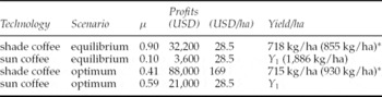
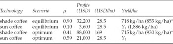
In this section, we compute the dominant equilibrium (small-scale farming) and the joint profits maximum (sole ownership) for our empirical data. Our base scenario uses the parameter values presented in tables A.1 and A.3 in Appendices A.2 and A.3, respectively. For these values, the dominant equilibrium is to allocate 90 per cent of the area to shade coffee production. The joint profits maximum that would maximize the total profits from the whole region is to allocate 41 per cent of the area to shade coffee. This means that when the farmers do not coordinate their decisions, they allocate a considerable amount of land to the more profitable (on average) technology, which proves to be shade coffee, given our initial parameter values. The main characteristics of the dominant equilibrium (small-scale farming) and the joint profits maximum (sole ownership) are summarized in table 1.
Characteristics of dominant equilibria and joint optima for base scenario
* yield/ha without the forest strip.
In the dominant equilibrium, the profitability of the two technologies is the same, whereas in the joint profits maximum the profitability of shade coffee is much higher than that of sun coffee. The size of the forest strip is 181 ha in the dominant equilibrium, and 120 ha in the joint profits maximum. The most striking difference is in the total profits, which are about USD 35,800 in the dominant equilibrium and USD 109,000 in the joint profits maximum. This is an interesting result. There seems to be a clear incentive for the small-scale farmers to coordinate their land allocation decisions to maximize their total economic benefits. In our model, this would lead to a further decrease in land area for shade coffee, down to 41 per cent according to our analysis. This would be a dramatic decrease, as historically only shade coffee has been cultivated. Recall, however, that coordination of land allocation decisions would enable the optimal design of forest patches, which might reduce the decrease in the area used for shade coffee production.
As there are many uncertainties related to the ecological data, we also report here a sensitivity analysis for selected key parameters of our model. We study how the dominant equilibrium changes when the minimum width of the forest strip (δ0) and the yield of sun coffee (Y 1) vary. As the forest strip surrounding a shade coffee region becomes narrower, the equilibrium allocation of shade coffee increases. When δ0 is less than 125 m, there is only shade coffee in the equilibrium. Doubling the width from 125 m to 250 m would decrease the land allocated to shade coffee by 34 per cent, from μ = 1 to μ = 0.66.
The critical price thresholds increase linearly when Y 1 increases. To exemplify the magnitude: if Y 1 is increased by 100 kg/ha, the resulting increase in the price premium above which there is only shade coffee is USD 0.125. The threshold below which there is only sun coffee behaves in approximately the same way, which is also the case for the equilibrium. If yields could be increased in sun coffee production, for instance, by 10 per cent, the price premium for shade coffee should increase about 23 per cent.
The dilemma for policy makers is that maximizing joint profits would be an efficient way to increase economic benefits and alleviate poverty. However, there are most likely additional environmental benefits from having more shade coffee production than a profit-maximizing optimum would provide. As there is not enough scientific knowledge for determining an ecologically optimal amount of shade coffee production (or forest), we compare the impacts of alternative policy instruments designed for promoting ecologically and economically sustainable farming practices. In the following, we shall focus on the impacts on the dominant equilibrium.
4.2. Comparison of policy instruments
To make the instruments comparable, we fix the budget expenditure for promoting sustainable farming practices. Any arbitrary sum of money could be chosen for comparison, and we assume that a donor spends USD 6/ha for the total production area under consideration (or a lump sum of 6 × 1,256 ≈ 7500). For the comparison to make sense in the case of minimum wage, we add the extra cost (due to increased minimum wages) in the equilibrium profits. For the price premium we assume that USD 6/ha is spent so that an extra premium is added to the base level, p 2−p 1. The base level changes, when we analyze the effect of decreasing the marginal price p 2−c 2.
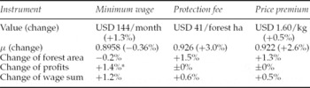
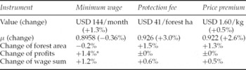
Table 2 summarizes the impacts of alternative policy instruments on the proportion of shade coffee production, μ, and forest area in the dominant equilibrium. Allocating funding through a price premium or a protection fee would increase both shade coffee and forest areas. In contrast, if the same amount of funding were spent on compensating for additional input costs or an increase in the wage rate for poor employees, the minimum wage could be increased by 1.3 per cent with only a negligible negative impact on forest conservation (−1 per cent). Social benefits, as measured by a wage sum, would favor the increase of the minimum wage as a policy instrument for the alleviation of poverty. This would come at the expense of ecological benefits, leading to a reduction in forested area in contrast to the other instruments, although the magnitude of the reduction would remain moderate.
Comparison of policy impacts when an additional payment of USD 6/ha is delivered through alternative policy instruments
* USD 6/ha added to profits.
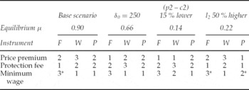
Let us now consider changes in the minimum width of the forest strip, δ0, the required labor months in shade coffee production, l 2, and the marginal price of shade coffee, p 2−c 2. We rank the instruments according to three criteria: the increase in forest area (F), wage sum (W), and profits (P). For example, in the base scenario the rankings of the price premium in these criteria are 2, 3, and 2, respectively, indicating that the price premium is the second best instrument in promoting forest area and profits, and the third best (worst) in increasing the wage sum. The rankings are collected in table 3.
Sensitivity of the ranking of policy instruments
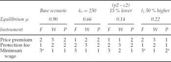
Rankings according to increase in forest area (F), wage sum (W), and profits (P).
* The instrument causes a decrease instead of an increase.
The most interesting finding here is that the price premium becomes a better instrument than the conservation fee when δ0 increases or when the marginal price p 2−c 2 decreases. The explanation is the same for both instruments. Due to large δ0 or, respectively, to small p 2−c 2, the equilibrium μ is small. When only a small area is allocated to shade coffee, pollination is highly effective. Consequently, the yield increases steeply for a small increase of μ. A higher price premium (p 2−p 1) of shade coffee generates more profits from the yield, whereas a higher conservation fee generates profits from the forest area in shade coffee production. For small initial μ, an increase causes a more dramatic increase in the yield than in the forest area. Therefore, the price premium increases the profitability of shade coffee more effectively than the protection fee. The ultimate impact of the price premium depends critically on the design of certification standards, i.e. the forest area required for protecting pollinator habitats.
From table 3, we observe that when the marginal price p 2−c 2 is decreased 15 per cent from its level in the base scenario, the price premium causes the highest increase in wages. The ranking of instruments is most sensitive to changes in p 2−c 2. Sensitivity to labor costs is less significant. These costs increase in the particular case when shade coffee production becomes more labor intensive, e.g. when l 2 increases 50 per cent as in table 3. As seen from table 3, the minimum wage becomes less effective compared to the other two instruments when the labor requirement l 2 increases. In particular, the minimum wage does not increase the farmers’ profits as well as the other instruments do even though the extra costs are compensated (USD 6/ha is added to profits). The two other instruments, on the other hand, keep their ranks relative to each other when l 2 increases.
5. Conclusions
Overuse of natural resources may be a direct consequence of poverty, given that a choice of farming practices typically involves a trade-off between short-term private benefits and a public good, biodiversity, or long-term sustainability in land use. By capturing the interaction between coffee yield and pollination services in an analytical bio-economic model, we have investigated the decline in biodiversity related to two alternative production methods, sun- and shade-grown coffee.
We examined the pattern of technology choice at the level of a representative local community by calibrating an empirical model using data on Costa Rica. We found that maintaining environmentally sustainable farming practices requires over-allocation of land to shade coffee production compared to levels that would be economically optimal. This results from an inability to coordinate management decisions when there are several economic agents involved, typically small-scale farmers. We assumed that small-scale farmers choose between shade and sun coffee based on the profitability of each technology. This leads to a dominant equilibrium where the profitability of each technology is the same, whereas in an economic optimum the marginal profits are equalized. In the dominant equilibrium, a smaller area of shade coffee would produce higher profits per hectare due to a better pollination effect. Following Klein et al. (Reference Klein, Steffan-Dewenter and Tscharntke2003c), we assumed that the yield of a plant decreases as a function of distance from the forest surrounding the shade coffee region. For a larger area of shade coffee, more plants are far away from the forest serving as the source of pollinating bees. This explains why in the dominant equilibrium allocating less land to shade coffee would increase the total profits and why the opportunity costs of shade coffee production are high.
We compared alternative policy instruments – price premiums, conservation fees, and minimum wages – and investigated whether it is possible to prevent loss of biodiversity and promote economic sustainability simultaneously. A direct conservation fee and a price premium are equally effective for achieving comparable positive economic and ecological impacts. Moreover, we expected a priori that increasing minimum wages would increase the relative profitability of sun coffee production at the expense of shade coffee, given that production of shade coffee is more labor intensive. However, we found this impact to be negligible in our analysis, and an increase in minimum wages could in fact be a stabilizing, robust policy instrument: it would not lead to a dramatic decrease in the forest area, and the positive economic impacts would be significant. One policy recommendation would then be that addressing economic sustainability first would not necessarily jeopardize biodiversity. Our results differ from those of Ferraro et al. (Reference Ferraro, Uchida and Conrad2005) and Ferraro and Simpson (Reference Ferraro and Simpson2002) to an extent, due to a different kind of tension between shade coffee and forest area in our case. The larger the required area of forest in shade coffee production the less productive and attractive technology shade coffee is.
One of our aims in the paper was to analyze whether price premium as an ‘in-between instrument’ would do better than conservation payments and minimum wages when simultaneously targeting both poverty and biodiversity. We found that price premium does better than protection fee in protecting biodiversity when the compulsory forest area associated with shade coffee is large. In such circumstances, price premium also outperforms minimum wage in promoting the wage sum (but not profits). Similarly, when the cost of labor is high, price premium outperforms minimum wage in promoting profits but not the wage sum. These results demonstrate the importance of accounting for trade-offs between different objectives and ensuring that when trying to reach one target we are not at the same time compromising other targets.