2.1. Governing equations and numerical methods

We conducted numerical simulations for explosive granular dispersal systems using the compressible multiphase particle-in-cell (CMP-PIC) method (Tian et al. Reference Tian, Zeng, Meng, Chen, Guo and Xue2020). This method integrates the Eulerian–Lagrangian approach to solve the motions of particles and gas. The two phases are fully coupled via volume fraction and momentum exchange terms, while the gas field surrounding the particle surfaces is not resolved (Capecelatro & Desjardins Reference Capecelatro and Desjardins2013). In the CMP-PIC method, a parcel for the particle phase consists of multiple particles with the same physical properties. The contribution of parcel $i$ to the weighted particle volume fraction is $\alpha _{p,i}=w_{i,c}V_{p,i}/V_{c}$ , where $V_{p,i}$ denotes the volume of parcel $i$ , $V_{c}$ the computational cell volume, and $w_{i,c}$ the distributed weight that parcel $i$ contributes to the particle volume fraction in each cell. The volume fraction of particles in a cell is $\alpha _{p}=\sum _{i}\alpha _{p,i}$ , and the volume fraction of gas is $\alpha _{\kern-1pt f}=1-\alpha _{p}$ .

The CMP-PIC method tracks parcels in the Lagrangian framework and takes parcel–parcel interactions into account. The motion of parcels is governed by

(2.1) \begin{align} \frac {\mathrm{D}\boldsymbol{x}_{p,i}}{\mathrm{D}t}=\boldsymbol{v}_{p,i} \end{align}

and

(2.2) \begin{align} \frac {\mathrm{D}\boldsymbol{v}_{p,i}}{\mathrm{D}t}=\boldsymbol{a}_{p,i}=\frac {1}{m_{p,i}}\sum _{j}\boldsymbol{F}_{C,\textit{ij}}-\boldsymbol{S}_{p,i}. \end{align}

Here, $\boldsymbol{a}_{p,i}$ , $m_{p,i}$ , $\boldsymbol{x}_{p,i}$ and $\boldsymbol{v}_{p,i}$ denote the acceleration, mass, location and velocity of parcel $i$ , respectively. The collision force

(2.3) \begin{align} \boldsymbol{F}_{C,\textit{ij}}=k_{n,p}\boldsymbol{\delta }_{n}+\frac {2\ln \epsilon _{p}}{\sqrt {\pi ^{2}+\ln ^2\epsilon _{p}}}\sqrt {m_{p,i}k_{n,p}}\boldsymbol{u}_{n,\textit{ij}} \end{align}

between parcels $i$ and $j$ is calculated by a soft-sphere model (Liu, Tafti & Li Reference Liu, Tafti and Li2014), where the stiffness $k_{n,p}$ and the restitution coefficient $\epsilon _{p}$ characterise parcel properties, and the overlap distance $\boldsymbol{\delta }_{n}$ with the normal velocity difference $\boldsymbol{u}_{n,\textit{ij}}$ describes contact dynamics between parcels.

The source term of parcel $i$ applied by the gas phase is

(2.4) \begin{align} \boldsymbol{S}_{p,i}=\frac {1}{\rho _{p}}\boldsymbol{\nabla }p_{\kern-1pt f}+D_{p,i}\big (\boldsymbol{v}_{p,i}-\boldsymbol{u}_{\kern-1pt f}\big ), \end{align}

with the particle density $\rho _{p}$ , gas pressure $p_{\kern-1pt f}$ and gas velocity $\boldsymbol{u}_{\kern-1pt f}$ . Here, the drag force coefficient

(2.5) \begin{align} D_{p,i}=C_d\frac {3\rho _f\big |\boldsymbol{v}_{p,i}-\boldsymbol{u}_{\kern-1pt f}\big |}{4\rho _pd_p} \end{align}

is calculated using the Di Felice model combined with Ergun’s equation (Crowe, Sommerfield & Tsuji Reference Crowe, Sommerfield and Tsuji1998), with the dimensionless drag coefficient

(2.6) \begin{align} C_{d}=\frac {24}{R e_{p}}\left \{\begin{array}{ll} 8.33 \dfrac {\alpha _{p}}{\alpha _{\kern-1pt f}}+0.0972 R e_{p}, &\alpha _{\kern-1pt f}\lt 0.8, \\[6pt] f_{\textit{base}} \alpha _{\kern-1pt f}^{-\zeta }, &\alpha _{\kern-1pt f} \geqslant 0.8, \end{array}\right . \end{align}

standard drag factor (McGrath, Clair & Balachandar Reference McGrath, Clair and Balachandar2016)

(2.7) \begin{align} f_{\textit{base}}=\left \{\begin{array}{cc} 1+0.167 \textit{Re}_{p}^{0.687}, &\textit{Re}_{p}\lt 1000, \\[6pt] 0.0183 \textit{Re}_{p}, &\textit{Re}_{p} \geqslant 1000, \end{array}\right . \end{align}

and the exponent

(2.8) \begin{align} \zeta =3.7-0.65 \exp \left [-\frac {1}{2}\left (1.5-\log _{10} \textit{Re}_{p}\right )^{2}\right ]. \end{align}

Here, $d_{p}$ is the particle diameter, $\rho _{\kern-1pt f}$ the gas density, $\mu _{\kern-1pt f}$ the gas viscosity, and ${\textit{Re}}_{p}=\rho _{\kern-1pt f}d_{p}\left |\boldsymbol{v}_{p,i}-\boldsymbol{u}_{\kern-1pt f}\right |/\mu _{\kern-1pt f}$ the particle Reynolds number. Note that specifying the valid range for the drag models is non-trivial (Osnes et al. Reference Osnes, Vartdal, Khalloufi, Capecelatro and Balachandar2023).

The inertial properties of particles in a fluid flow is characterised by the Stokes number

(2.9) \begin{align} {St}=\tau _{p}/\tau _{f}, \end{align}

where the particle response time

(2.10) \begin{align} \tau _{p}=\frac {\rho _{p}d_{p}^2}{18\mu_{\kern-2pt f} \left (1+0.15{\textit{Re}}_{p}^{0.687}\right )} \end{align}

is evaluated using the Schiller–Naumann correction (Berk & Coletti Reference Berk and Coletti2021), and the flow field characteristic time

(2.11) \begin{align} \tau _{f}=\frac {L_{\tau }}{V_{\tau }} \end{align}

is the ratio of the characteristic length $L_{\tau }$ to the characteristic velocity $V_{\tau }$ in the flow field.

The gas phase in CMP-PIC is discretised in the Eulerian framework using four-way coupling (Wang, Liu & Yang Reference Wang, Liu and Yang2020). This approach extends the two-way coupling method (Barba & Picano Reference Barba and Picano2018) by additionally accounting for particle–particle collisions and the influence of particle volume fraction on the gas, while maintaining the momentum and energy transfers between gas and particles. The gas-phase governing equations (Shallcross, Fox & Capecelatro Reference Shallcross, Fox and Capecelatro2020)

(2.12) \begin{align} \frac {\mathrm{D} \left (\alpha _{\kern-1pt f}\rho _{\kern-1pt f}\right )}{\mathrm{D}t}=-\alpha _{\kern-1pt f}\rho _{\kern-1pt f}\left (\boldsymbol{\nabla }\boldsymbol{\cdot }\boldsymbol{u}_{\kern-1pt f}\right ), \\[-28pt] \nonumber \end{align}

(2.13) \begin{align} \frac {\mathrm{D} \left (\alpha _{\kern-1pt f}\rho _{\kern-1pt f}\boldsymbol{u}_{\kern-1pt f}\right )}{\mathrm{D}t}=-\alpha _{\kern-1pt f}\rho _{\kern-1pt f}\boldsymbol{u}_{\kern-1pt f}\left (\boldsymbol{\nabla }\boldsymbol{\cdot }\boldsymbol{u}_{\kern-1pt f}\right )-\alpha _{\kern-1pt f}\boldsymbol{\nabla }p_{\kern-1pt f}+\sum _{i}\rho _{p,i}\alpha _{p,i}\boldsymbol{S}_{p,i}, \\[-28pt] \nonumber \end{align}

(2.14) \begin{align} \frac {\mathrm{D}\left (\alpha _{\kern-1pt f}\rho _{\kern-1pt f}E_{\kern-1pt f}\right )}{\mathrm{D}t}=-\alpha _{\kern-1pt f}\rho _{\kern-1pt f}E_{\kern-1pt f}\left (\boldsymbol{\nabla }\boldsymbol{\cdot }\boldsymbol{u}_{\kern-1pt f}\right )-\boldsymbol{\nabla }\boldsymbol{\cdot }\left (\alpha _{\kern-1pt f}p_{\kern-1pt f}\boldsymbol{u}_{\kern-1pt f}\right )+\sum _{i}\rho _{p,i}\alpha _{p,i}\boldsymbol{S}_{p,i}\boldsymbol{\cdot }\boldsymbol{v}_{p,i} \\[-12pt] \nonumber \end{align}

are simplified from the model of Baer & Nunziato (Reference Baer and Nunziato1986), where $\rho_{p,i}$ is the density of parcel $i$ , the subscript $i$ denotes the parcel $i$ and $E_{\kern-1pt f}=e+ (\boldsymbol u_{f}\boldsymbol{\cdot }\boldsymbol u_{f} )/2$ denotes the total energy of gas per unit volume. They are closed with the equation of state for ideal gas

(2.15) \begin{align} p_{\kern-1pt f}=\rho _{\kern-1pt f}\frac {\mathcal{R}}{M}T=\rho _{\kern-1pt f} e\left (\gamma -1\right ), \end{align}

with the gas density $\rho _{\kern-1pt f}$ , ideal gas constant $\mathcal{R}$ , molar mass $M$ , temperature $T$ , specific heat ratio $\gamma =C_{p}/C_{v}$ and internal energy $e$ . Here $ C_p $ and $ C_v $ is the specific heat at constant pressure and constant volume respectively.

The CMP-PIC has been validated against several benchmark experiments involving shock-driven particle-laden flows (Tian et al. Reference Tian, Zeng, Meng, Chen, Guo and Xue2020), including Rogue’s experiments (Rogue et al. Reference Rogue, Rodriguez, Haas and Saurel1998), the experiments conducted by Britan & Ben-Dor (Reference Britan and Ben-Dor2006), the cavity formation in granular media due to explosions (Zeng et al. Reference Zeng, Meng, Ye and Tian2024) and the experiments of shock-induced interfacial instability of granular media (Xue et al. Reference Xue, Du, Shi, Gan and Bai2018).

2.2. Simulation set-up

As sketched in figure 1(a), we consider a 2-D problem – a high-pressure gas pocket with radius $R_{g}$ expands the surrounding particle bed with initial inner radius $R_{I0}$ and outer radius $R_{O0}$ . This problem is simulated in the domain $\mathcal{D}= [0,W_{x} ]\times [0,W_{y} ]$ , with domain sizes $W_x$ and $W_y$ in the $x$ - and $y$ -directions. Both the gas pocket and the particle bed are set at the domain centre $(x_c,y_c)=(W_{x}/2,W_{y}/2)$ . The cylindrical coordinate $(r,\theta )$ is related to the Cartesian coordinate $(x,y)$ as $r=((x-x_c)^2+(y-y_c)^2)^{1/2}$ and $\theta =\arctan (y-y_c,x-x_c)$ . The high-pressure gas pocket is filled with still air with pressure $P_{s}$ , density $\rho _{s}$ and temperature $T_{s}$ . For the still air, we set the initial ambient pressure $P_0=1.013\times 10^5\,\rm {Pa}$ , temperature $T_0=299.5\,\rm {K}$ and density $\rho _{0}=P_0 M_{\textit{air}}/ (\mathcal{R}T_0 )$ with the species molar mass $M_{\textit{air}}=29\,\mathrm{g}\,\mathrm{mol^{-1}}$ . The radius and temperature of the gas pocket are set as $R_{g}=20\,\mathrm{mm}$ and $T_{s}=299.5\,\mathrm{K}$ , respectively. Thus, the equation of state for ideal gas in (2.15) gives $\rho _s/\rho _0=P_s/P_0$ . Note that the high-pressure gas serves as the simulant agent for cylindrical bursters (Xue et al. Reference Xue, Miu, Li, Bai and Tian2023).

Figure 1.

(a) Schematic of the 2-D explosive dispersal system set-up in the numerical simulation. The red circular area denotes the gas pocket with high pressure. The grey circles denote the particle bed. (b) Schematic for the external particle jet growth with the initial random perturbation (upper row) and the single-mode perturbation (lower row). The particle bed (grey circles) is enclosed by the red dashed line. The region is shaded based on pressure (darker areas indicate higher pressure). The blue and black arrows represent the radial flow and particle velocities, respectively.

The annular particle bed with initial volume fraction $\varPhi _0=0.6$ is filled by random distributed computational parcels (Lozano et al. Reference Lozano, Roehl, Celes and Gattass2016). The diameter of the parcel is set to range uniformly from $450$ to $750\,\mathrm{\unicode {x03BC} m}$ to avoid potential crystallisation during shock compaction (Xue et al. Reference Xue, Miu, Li, Bai and Tian2023). Note that convergence is observed as the number of particles per parcel decreases, and a single realisation is sufficient for the statistics of the particle jet length. The particle diameter $d_{p}=100\,\unicode {x03BC}\mathrm{m}$ and gas viscosity $\mu _{\kern-1pt f}=1.92\times 10^{-5}\,\mathrm{Pa\,s}$ are used to calculate the particle drag force in (2.5). The restitution coefficient $\epsilon _{p}=0.6$ and the normal stiffness $k_{n,p}=5.0\times 10^{6}\,\mathrm{N\,m^{-1}}$ of contacts between parcels for calculating the particle collision force are set in (2.3). The restitution coefficient $0.9$ and normal stiffness $O(10^{6})\,\mathrm{N\,m^{-1}}$ of real particles within the parcels (Renzo, Napolitano & Maio Reference Renzo, Napolitano and Maio2021) correspond to those of glass beads.

The constant initial inner radius $R_{I0}=40\,\mathrm{mm}$ of the particle bed is set with the thickness $h=R_{O0}-R_{I0}$ . The outer interface of the particle bed is parametrised as $r=R_{O0}+a_{i0}\cos (n\theta )$ , with the number $n$ of azimuthal modes and the initial amplitude $a_{i0}$ of the outer interface. The mass ratio between the surrounding particles and the gas pocket (Xue et al. Reference Xue, Miu, Li, Bai and Tian2023) is

(2.16) \begin{align} \varGamma _M=\frac {\pi \left (R_{O0}^2-R_{I0}^2\right )\varPhi _0\rho _p}{\pi R_{g}^2\rho _{s}}. \end{align}

The sound speed of air $c_{s}=\sqrt {\gamma P_{0}/\rho _{0}}$ and $h$ are used as the characteristic velocity $V_{\tau }$ and length $L_{\tau }$ of the flow field, respectively, to calculate the Stokes number. Substituting ${\textit{Re}}_{p}=\rho _{0}d_{p}c_{s}/\mu _{\kern-1pt f}$ , (2.11) and (2.10) into (2.9) yields ${\textit{Re}}_{p}=2150$ and $\textit{St}=O (10 )$ , indicating the heavy particles here have a large inertial force compared with the drag (Li, Zeng & Xue Reference Li, Wang, Zhai and Luo2023a ). The maximum particle Mach number $\textit{Ma}_{p}=\left |\boldsymbol{v}_{p,i}-\boldsymbol{u}_{\kern-1pt f}\right |/c_{s}$ is approximately $1.5$ in the present study. The multiphase Atwood number $A_{m}$ of the cases considered here is $-1$ (see (4.6)).

Two types of simulation cases, with random and single-mode perturbations, will be studied in the present study. For the random perturbation cases, we set $a_{i0}=0\,\mathrm{mm}$ , and only vary $P_{s}$ and $h$ . For the single-mode perturbation cases, we set $P_{s}=20\,\mathrm{bar}$ and $h=50\,\mathrm{mm}$ , and only vary $n$ and $a_{i0}$ . With grid convergence tests on the external particle jet length, the 2-D computational domain is discretised on $480\times 480$ uniform grid points with mesh spacing $\Delta x=1.04\,\mathrm{mm}$ . Note that due to the 2-D configuration, the volume of particle and computational cell are calculated as $\pi d_{p}^2/4$ and $\Delta x^2$ , respectively. Each parcel corresponds to $O (100 )$ particles, and over five million particles are tracked in each case. The time stepping $\Delta t$ is chosen to satisfy both the Courant–Friedrichs–Lewy condition and the time-step limit of the discrete element method (Tian et al. Reference Tian, Zeng, Meng, Chen, Guo and Xue2020). The third-order Runge–Kutta method is applied for the time integration.

The evolution of the external particle jet length is sketched in figure 1(b). The high-pressure gas pocket first compacts and accelerates the particle bed to a radial velocity $V_a$ . The compacted particle ring inhibits atmospheric air penetration into its internal region. In the random perturbation cases (upper row), the external particle jet exhibits a spike-like structure at its top and a bubble-like structure near its bottom. As the radially expanding particle bed reduces the gas pressure inside the particle bed to below atmospheric pressure, particles near the bubble are subject to a strong radially inward gas–particle coupling force and decelerate to a radial velocity $V_c$ . Meanwhile, the particles in the spike still move with $V_a$ . Under this velocity difference $V_a - V_c$ , the length of the external particle jet in the random perturbation cases grows to $L_{\textit{jr}}$ .

In the single-mode perturbation case (lower row of figure1 b), the pressure perturbation induced by the single-mode perturbation adds a radial velocity $V_{\textit{RM}}$ to the particles near the trough. Note that the trough-near particles accelerate to move faster than the crest-near particles, and then causes ‘phase inversion’ (Li et al. Reference Li, Ding, Si and Luo2020). Then the external particle jet length in the single-mode perturbation cases grows to $L_{\textit{js}} \gt L_{\textit{jr}}$ due to the additional $V_{\textit{RM}}$ .

3.1. Evolution of the external particle jet length

The contour plot of gas pressure and position of the computational parcels are shown in figure 2. The gas pressure in the central zone decreases and the particle bed expands at $t=2.9\,\mathrm{ms}$ in both the random and single-mode perturbation cases. Similar to the classical RMI of a heavy–light interface in cylindrical geometry (Li et al. Reference Li, Wang, Zhai and Luo2023a ), the single-mode perturbation case finishes the phase inversion, marked by the perturbation decreasing to zero, at approximately $t=2.9\,\mathrm{ms}$ . After the gas pressure in the central zone decreases to lower than the ambient pressure, the particle jet grows at $t=10.0\,\mathrm{ms}$ in both cases. The single-mode perturbation shows a dominant-particle-jet mode protruding from the trough of the outer interface, initially near $r=R_{O0}-a_{i0}$ as in (3.9), whereas a multi-mode external particle jet grows in the random perturbation case.

Figure 2.

Evolution of the particle bed (dots) and the pressure fields (contours) in (a) the random perturbation case with $P_{s}=20\,\mathrm{bar}$ and $h=50\,\mathrm{mm}$ and (b) the single-mode perturbation case with $n=12$ and $a_{i0}=2.4\,\mathrm{mm}$ . The radius of the green, blue and red circles indicate the inner radius $R_{I}$ of the particle bed, the outer radius $R_{C}$ of the particle bed and the outer radius $R_{O}$ of the jet zone, respectively. The numbers in the upper right corner denote the time in $\mathrm{ms}$ . The unit of the axes is $\mathrm{m}$ .

To quantify the external particle jet length, we measure characteristic radii with circumferentially averaged particle volume fractions $\bar {\alpha }_p(r)=\int _{0}^{2\pi }\alpha _{p}(r,\theta )\rm d\theta /(2\pi )$ . The threshold values for the inner radius $R_{I}$ of the particle bed, the outer radius $R_{C}$ of the particle bed and the outer radius of the jet zone $R_{O}$ are $\bar {\alpha }_p(r)=\alpha _{\textit{ps}}$ , $\bar {\alpha }_p(r)=\varPhi _0-\alpha _{\epsilon }$ and $\bar {\alpha }_p(r)=\alpha _{\epsilon }$ , $\alpha_{ps}$ and $\alpha_{\epsilon}$ represent the threshold values of particle volume fraction on the inner side and outer side of the particle bed, respectively. Here, $\alpha _{\textit{ps}}=0.1$ is set for measuring the inner side of the particle bed (Rana et al. Reference Rana, Abadie, Chapman, Joiner and Matar2024), and $\varPhi _0=0.6$ and $\alpha _{\epsilon }=0.01$ are set in all the cases. The dashed circles in figure 2 demonstrate that the characteristic radii capture the structures of the particle bed and the external particle jet well.

Figure 3 plots the evolution of characteristic radii. When high-pressure gases are released from the gas pocket, an incident shock wave impinges on the inner surface of the particle bed, resulting in a linear growth of $R_{I}$ , perturbed shock waves and a compaction front traversing the particle bed. The amplitude of the perturbed shock waves is comparable to the particle size. The oscillation frequency for the perturbed shock is given by $\omega _{s}=k_{s}c^{+}\sqrt {1-M^{+2}}$ (Huete et al. Reference Huete, Velikovich, Martinez-Ruiz and Calvo-Rivera2021), where $k_s$ denotes the wavenumber, and $c^{+}$ and $M^{+}$ represent the post-shock speed of sound and Mach number, respectively. For the random perturbation case with $P_{s}=20\,\mathrm{bar}$ and $h=50\,\mathrm{mm}$ , the oscillation period $T_{s}=2\pi /\omega _{s}$ for the perturbed shock is approximately $0.2\,\unicode {x03BC} \mathrm{s}$ by adopting $k_s=2\pi /d_p$ , $c^{+}=500\,\mathrm{m\,s^{-1}}$ and $M^{+}=0.1$ . The time interval for the shock passing through the particle bed is approximately $100\,\unicode {x03BC}\mathrm{s}$ , exceeding the oscillation period by two orders of magnitude. Consequently, the perturbed amplitude of the incident shock introduced by randomly distributed particles rapidly diminishes. After the compaction front reaches the outer surface of the particle bed at approximately $t=2\,\mathrm{ms}$ , $R_{O}$ and $R_{C}$ start to grow. In both the random and single-mode perturbation cases, $R_{C}$ experiences a short period of linear growth and the growth is mitigated at approximately $t=3\,\mathrm{ms}$ due to strong inward gas–particle coupling forces. Moreover, the evolutionary trends of $R_{I}$ , $R_{O}$ and $R_{C}$ are very similar in both cases.

Figure 3.

Evolution of characteristic radii in the random perturbation case with $P_{s}=20\,\mathrm{bar}$ and $h=50\,\mathrm{mm}$ (solid lines) and the single-mode perturbation case with $n=12$ and $a_{i0}=2.4\,\mathrm{mm}$ (dashed lines).

The external particle jet length

(3.1) \begin{align} L_{j\varPsi }=R_{O}-R_{C},\,\,\,\varPsi =r, s \end{align}

is defined as the outer radius difference between the particle bed and the top of the jet, where subscripts $r$ and $s$ denote the random and single-mode perturbation cases, respectively. The evolution of $L_{\textit{jr}}$ and $L_{\textit{js}}$ is plotted in figure 4. All the random and single-mode perturbation cases undergo a compression stage until the critical time $t=t_c$ , when the jet length reaches its minimum value. They then enter a nonlinear growth stage. In the random perturbation cases, $L_{\textit{jr}}$ grows faster with larger $P_s$ and smaller $h$ . This is because the particle bed expands more rapidly under these conditions, accelerating $R_O$ and causing a quicker decline in $p_f$ in the central zone, which in turn strongly decelerates the growth of $R_C$ . In the single-mode perturbation cases, $L_{\textit{js}}$ grows faster with larger $n$ and $a_{i0}$ because faster growth of $R_{O}$ results from stronger pressure perturbations induced by the larger $n$ and $a_{i0}$ . The effects of parameters on $L_{\textit{jr}}$ and $L_{\textit{js}}$ will be discussed further in § 4.

Figure 4.

Evolution of the particle jet length in (a) the random perturbation cases and (b) the single-mode perturbation cases with various parameters.

To investigate the single-mode perturbation’s effects on the growth of the particle jet length, we introduce the jet length increment $\Delta L_{j}=L_{\textit{js}}-L_{\textit{jr}}^*$ , where $L_{\textit{jr}}^*$ and $L_{\textit{js}}$ denote the particle jet length of the random perturbation case with $P_{s}=20\,\mathrm{bar}$ and $h=50\,\mathrm{mm}$ and the single-mode perturbation cases with the same $P_{s}$ and $h$ , respectively. In figure 5, $\Delta L_{j}$ firstly experiences the compression stage because the particles initially near the trough accelerate to move faster than those initially near the crests. After the phase inversion at $t=t_m$ (listed in table 1), $\Delta L_{j}$ experiences a linear growth, which is similar to that observed in the linear stage of planar RMI (Richtmyer Reference Richtmyer1960; Meshkov Reference Meshkov1969) and is distinct from the nonlinear growth of the cylindrical RMI (Bell Reference Bell1951; Mikaelian Reference Mikaelian2005; Ding et al. Reference Ding, Si, Yang, Lu, Zhai and Luo2017).

Table 1.

Summary of parameters in random and single-mode perturbation cases. Additionally, $R_{I0}=40\,\mathrm{mm}$ , $R_{g0}=20\,\mathrm{mm}$ and $\varPhi _{0}=0.6$ are set in all cases. The wave number is $k=n/R_{O0}$ .

Figure 5.

Evolution of the particle jet length increment in the single-mode perturbation cases with various parameters.

3.2. Formation of the external particle jet

As sketched in figure 6(a), we measure the averaged particles’ quantities at the compaction (C) zone within $R_C-0.1h\lt r\lt R_C$ and near the outer (O) zone within $|r_{0}-R_{O0}|\lt \Delta x$ to characterise the external particle jet growth, where $r_0$ denotes the radial coordinate $r$ at the initial time $t = 0$ . The random perturbation case with $P_{s}=20\,\mathrm{bar}$ and $h=50\,\mathrm{mm}$ is studied here. We calculate the mass-weighted averaged radial components of coordinate, velocity and acceleration

(3.2) \begin{align} \bar {f}_{\textit{pr},\varOmega }=\frac {\sum _{i\in \varOmega }\rho _{p}\alpha _{p,i}f_{\textit{pr},i}}{\sum _{i\in \varOmega }\rho _{p}\alpha _{p,i}}, \,\,\,f=r,v,a\,\text{and}\, \varOmega ={C, O} \end{align}

of particles at the compaction and outer zones, where $\rho _{p}$ and $\alpha _{p,i}$ are the particle density and particle volume fraction, respectively.

Figure 6.

(a) Evolution of particles in the random perturbation case with $P_{s}=20\,\mathrm{bar}$ and $h=50\,\mathrm{mm}$ . The red and blue dots represent particles in the outer and compaction zones, respectively. (b) Evolution of the characteristic radii (symbols) and the radii integrated from the averaged velocity of the outer and compaction zones (lines).

Figure 6(b) shows that the radii

(3.3) \begin{align} \hat {R}_{\textit{pr},\varOmega }(t)=\bar {r}_{\textit{pr},\varOmega }(t=0)+\int _{0}^{t}\bar {v}_{\textit{pr},\varOmega }(\tau)\mathrm{d}\tau ,\,\,\,\varOmega ={C, O} \end{align}

integrated from the average velocity of the compaction and outer zones are close to the characteristic radii, i.e. $\hat {R}_{\textit{pr},\varOmega }\approx R_{\varOmega }$ . Thus, the growth rate

(3.4) \begin{align} \frac {\mathrm{d}L_{\textit{jr}}}{\mathrm{d}t}=\frac {\textit{d}\left (R_{O}-R_{C}\right )}{\mathrm{d}t}\approx \frac {\textit{d}\big (\hat {R}_{\textit{pr},O}-\hat {R}_{pr,C}\big )}{\mathrm{d}t}=\bar {v}_{\textit{pr},O}-\bar {v}_{pr,C} \end{align}

of the external particle jet length can be approximated as the difference between average radial velocities of particles in compaction and outer zones.

According to (3.4), we further study the evolution of $\bar {v}_{\textit{pr},O}$ and $\bar {v}_{pr,C}$ . Figure 7(a) shows that the velocities

(3.5) \begin{align} \hat {v}_{\textit{pr},\varOmega }(t)=\bar {v}_{\textit{pr},\varOmega } (t=0)+\int _{0}^{t}\bar {a}_{\textit{pr},\varOmega }(\tau)\mathrm{d}\tau ,\,\,\,\varOmega ={C, O} \end{align}

integrated from the averaged accelerations agree well with the averaged velocities $\bar {v}_{\textit{pr},O}$ and $\bar {v}_{pr,C}$ . From (2.2), the $r$ -acceleration of parcel $i$ is contributed from the drag, pressure and collision as

(3.6) \begin{align} \begin{aligned} a_{\textit{pr}, i}=\underbrace {\vphantom {\frac {1}{m_{p,i}}\sum _{j}F_{\textit{Cr},\textit{ij}}}D_{p,i}\left (\boldsymbol{v}_{\textit{pr},i}-\boldsymbol{u}_{fr}\right )}_{\textit{Drag},\,a_{\textit{idr}}}\underbrace {\vphantom {\frac {1}{m_{p,i}}\sum _{j}F_{\textit{Cr},\textit{ij}}}-\frac {1}{\rho _{p}}\partial _{r} p_{\kern-1pt f}}_{\textit{Pressure},\,a_{\textit{ipr}}}+\underbrace {\frac {1}{m_{p,i}}\sum _{j}F_{\textit{Cr},\textit{ij}}}_{\textit{Collision},\,a_{\textit{icr}}}. \end{aligned} \end{align}

Thus, the mass-weighted averaged acceleration of particles in the outer and compaction zones can be rewritten as

(3.7) \begin{align} \bar {a}_{\textit{pr}, \varOmega }(t)=\bar {a}_{\textit{idr},\varOmega }+\bar {a}_{\textit{ipr},\varOmega }+\bar {a}_{\textit{icr},\varOmega },\,\,\,\varOmega ={C, O}, \end{align}

then the integrating velocity $\hat {v}_{pr}$ in (3.5) can be decomposed as

(3.8) \begin{align} \hat {v}_{\textit{pr}, \varOmega }(t)=\underbrace {\int _{0}^{t}\bar {a}_{\textit{idr},\varOmega }\,\mathrm{d}t}_{{drag},\,\hat {v}_{\textit{idr}}}+\underbrace {\int _{0}^{t}\bar {a}_{\textit{ipr},\varOmega }\,\mathrm{d}t}_{\textit{pressure},\,\hat {v}_{\textit{ipr}}}+\underbrace {\int _{0}^{t}\bar {a}_{\textit{icr},\varOmega }\,\mathrm{d}t}_{\textit{collision},\,\hat {v}_{\textit{icr}}},\,\,\,\varOmega ={C, O}, \end{align}

with $\bar {v}_{\textit{pr},\varOmega } (t=0 )=0$ .

Figure 7.

(a) Comparisons of the averaged velocity $\bar {v}_{pr}$ in (3.2) and integrating velocity $\hat {v}_{pr}$ in (3.5) in the random perturbation case with $P_{s}=20\,\mathrm{bar}$ and $h=50\,\mathrm{mm}$ . (b) Evolution of budgets of $\hat {v}_{pr}$ in the outer zone (dashed lines) and compaction zone (solid lines).

Figure 7(b) plots the evolution of budgets of $\hat {v}_{pr}$ . In the compaction zone, the pressure and drag terms first increase $\hat {v}_{pr,C}$ before $t=2.9\,\mathrm{ms}$ , and then decrease $\hat {v}_{pr,C}$ dramatically. Thus, particles in the compaction zone experience strong inward gas–particle coupling forces and undergo RTI with variable acceleration. In addition, the collision term has negligible effects on the variation of $\hat {v}_{pr,C}$ before $t=2.9\,\mathrm{ms}$ , and then increases $\hat {v}_{pr,C}$ .

In the outer zone, the pressure and collision terms first increase $\hat {v}_{\textit{pr},O}$ before $t=2.9\,\mathrm{ms}$ , and then they have negligible effects on the variation of $\hat {v}_{\textit{pr},O}$ , due to the large particle inertia and small particle volume fraction, respectively. In addition, the drag term increases $\hat {v}_{\textit{pr},O}$ before $t=2.9\,\mathrm{ms}$ , and then slightly decreases $\hat {v}_{\textit{pr},O}$ . Thus, RTI controls radial deceleration in the compaction zone, while large particle inertia keeps near-constant radial velocity in the outer zone, enabling faster movement of outer particles and promoting external jet growth.

3.3. Effects of RMI on the jet length increment

Since the growth of jet length increment is analogous to that of planar RMI (Peng, Yang & Xiao Reference Peng, Yang, Wu and Xiao2021a , Reference Peng, Yang and Xiao2021b ), we examine the effects of RMI on the jet length increment. To investigate the contributions of RMI on the particle jet growth, we track the motion of particles, which are initially near the trough (T) and waist (W) points. The trough, waist and crest points (see figure 1) are at the radial coordinates

(3.9) \begin{align} r_{T}=R_{O0}-a_{i0},\,\,\,\theta _{T}=\frac {\left (2i+1\right )\pi }{n},\,\,\,i=0,\ldots ,n-1, \\[-28pt] \nonumber \end{align}

(3.10) \begin{align} r_{W}=R_{O0},\,\,\,\theta _{W}=\frac {\left (4i\pm 1\right )\pi }{2n},\,\,\,i=0,\ldots ,n-1 \\[6pt] \nonumber \end{align}

and

(3.11) \begin{align} r_{\textit{crest}}=R_{O0}+a_{i0},\,\,\,\theta _{\textit{crest}}=\frac {2i \pi }{n},\,\,\,i=0,\ldots ,n-1, \end{align}

respectively. The waist-near particles satisfy $|r_{0}-r_{W}|\lt \Delta x$ and $\left |\theta _{0}-\theta _{W}\right |\lt 0.01\pi$ . The trough-near particles are initially in the disk region of radius $R_{TN}=\Delta x$ centring at the trough point. The single-mode perturbation case with $n=12$ and $a_{i0}=2.4\,\mathrm{mm}$ is studied here. The mass-weighted averaged radial components of coordinate, velocity and acceleration

(3.12) \begin{align} \bar {f}_{\textit{pr},\varOmega }=\frac {\sum _{i\in \varOmega }\rho _{p}\alpha _{p,i}f_{\textit{pr},i}}{\sum _{i\in \varOmega }\rho _{p}\alpha _{p,i}}, \,\,\,f=r,v,a\,\text{and}\, \varOmega ={T, W}, \end{align}

of the trough-near (T) and waist-near (W) particles are calculated.

Figure 8.

(a) Evolution of particles in the single-mode perturbation case with $n=12$ and $a_{i0}=2.4\,\mathrm{mm}$ . The initially trough-near (red dots) and waist-near (blue dots) particles are tracked in a Lagrangian framework. (b) Evolution of the jet length increment $\Delta L_{j}$ (symbols) and $\bar {r}_{pr,T}-\bar {r}_{pr,W}$ (lines).

The jet length can be represented by $\bar {r}_{pr,T}$ and $\bar {r}_{pr,W}$ . Figure 8(a) shows that the trough-near particles (red dots) are at the outermost part of the particle ring during $t\gt 2.9\,\mathrm{ms}$ , i.e. $R_O\approx \bar {r}_{pr,T}$ during the growth stage. Thus, combining with (3.1), the jet length in the single-mode perturbation case with $n=12$ and $a_{i0}=2.4\,\mathrm{mm}$ can be rewritten as

(3.13) \begin{align} L_{\textit{js}}\approx \bar {r}_{pr,T}-R_{C}=\left (\bar {r}_{pr,T}-\bar {r}_{pr,W}\right )+\left (\bar {r}_{pr,W}-R_C\right ). \end{align}

Meanwhile, the definition of $\Delta L_{j}$ suggests

(3.14) \begin{align} L_{\textit{js}}=\Delta L_{j}+L_{\textit{jr}}^{*} \end{align}

in the random perturbed case with $P_{s}=20\,\mathrm{bar}$ and $h=50\,\mathrm{mm}$ . Figure 8(b) shows that $\bar {r}_{pr,T}-\bar {r}_{pr,W}\approx \Delta L_{j}$ , hence the radial velocity difference between the trough-near and waist-near particles induced by the single-mode perturbation increases $\Delta L_{j}$ . Besides, the variation rate of $\Delta L_{j}$ is approximated by

(3.15) \begin{align} \Delta \dot {L}_{j} = \mathrm{d}\Delta L_{j}/\mathrm{d}t \approx \dot {\bar {r}}_{pr,T}-\dot {\bar {r}}_{pr,W}=\bar {v}_{pr,T}-\bar {v}_{pr,W}. \end{align}

Thus, we need to further study the evolution of $\bar {v}_{pr,T}$ and $\bar {v}_{pr,W}$ .

Figure 9(a) shows that both $\bar {v}_{pr,T}$ and $\bar {v}_{pr,W}$ accelerate before $t=2.9\,\mathrm{ms}$ , then decelerate slightly due to the large particle inertia. During the acceleration stage, the trough-near particles accelerates to move faster than the waist-near and crest-near particles, and then cause phase inversion.

The mass-weighted averaged velocity of the trough-near and waist-near particles can be rewritten as (He et al. Reference He, Meng, Tian and Yang2024)

(3.16) \begin{align} \bar {v}_{\textit{pr}, \varOmega }(t)=\bar {v}_{\textit{idr},\varOmega }+\bar {v}_{\textit{ipr},\varOmega }+\bar {v}_{\textit{icr},\varOmega },\,\,\,\varOmega ={T, W}, \end{align}

where $\bar {v}_{\textit{idr},\varOmega }$ , $\bar {v}_{\textit{ipr},\varOmega }$ and $\bar {v}_{\textit{icr},\varOmega }$ denote the drag, pressure and collision terms, respectively, and $\bar {v}_{\textit{pr},\varOmega }=0$ at $t=0$ .

Combining (3.15) and (3.16) yields the decomposition

(3.17) \begin{align} \Delta \dot {L}_{j}= \delta \bar {v}_{r}=\underbrace {\left (\bar {v}_{\textit{idr},T}-\bar {v}_{\textit{idr},W}\right )}_{\textit{Drag},\,\delta \bar {v}_{\textit{idr}}} -\underbrace {\left (\bar {v}_{\textit{ipr},T}-\bar {v}_{\textit{ipr},W}\right )}_{\textit{Pressure},\,\delta \bar {v}_{\textit{ipr}}} +\underbrace {\left (\bar {v}_{\textit{icr},T}-\bar {v}_{\textit{icr},W}\right )}_{\textit{Collision},\,\delta \bar {v}_{\textit{icr}}}, \end{align}

where $\delta$ denotes the velocity difference at the trough and waist. Figure 9(b) plots the evolution of budgets of $\delta \bar {v}_{r}$ . During the acceleration stage before $t=2.9\,\mathrm{ms}$ , the velocity difference $\delta \bar {v}_{r}$ is mainly contributed from collision and pressure terms. At the late stage, the drag term slightly increases $\delta \bar {v}_{r}$ due to large particle inertia. Due to the small particle volume fraction near the spike, the effects of the collision and pressure on $\delta \bar {v}_{r}$ is minor at the late stage. Therefore, the jet length increment (shown in figure 5) grows nearly linearly primarily because of the large particle inertia and small particle volume fraction.

Since the collision and pressure terms dominate the generation of $\delta \bar {v}_{r}$ , the gas–particle mixture can be viewed as a continuum during the acceleration stage. Thus, the single-mode perturbation triggers RMI, generating $\delta \bar {v}_{r}$ and $\Delta L_{j}$ . Note that the RMI in the random perturbation cases is negligible due to the small initial interfacial amplitude. The mode coupling effects on jet formation are discussed in Appendix A.

Figure 9.

Evolution of (a) the averaged velocity $\bar {v}_{r}$ of trough-near and waist-near particles and (b) budgets of $\delta \hat {v}_{r}$ in the single-mode perturbation case with $n=12$ and $a_{i0}=2.4\,\mathrm{mm}$ .

4.1. Jet-length-increment model

Inspired by the mechanism of the interfacial instability, we model the linear growth rate of the jet length increment. Richtmyer (Reference Richtmyer1960) developed a

(4.1) \begin{align} \dot {a}_{i}=ka_{i0}^{+}A^{+}\Delta U \end{align}

for a gas interface with perturbation amplitude $a_{i}$ subjected to a shock, where $a_{i0}^{+}$ , $A^{+}$ and $\Delta U$ are the post-shock perturbed amplitudes of the interface, Atwood number and average velocity difference of the gas around the interface, respectively. Ukai, Balakrishnan & Menon (Reference Ukai, Balakrishnan and Menon2010) developed a linear-growth model

(4.2) \begin{align} \dot {a}_{i}=ka_{i0}A_{m}\Delta U \end{align}

for the gas-phase interface surrounded by particles subjected to a shock, with introducing the multiphase Atwood number $A_{m}$ . Throughout the growth of external particle jets, the particle Mach number ${Ma}_{p}$ maintains values below $0.4$ , demonstrating negligible compressibility effects during this stage (Loth Reference Loth2008). Here we treat the gas–particle mixture as a continuum, and then propose a linear-growth model (detailed derivations are provided in Appendix B)

(4.3) \begin{align} \Delta \dot {L}_{j}=\dot {a}_{i}=ka_{i0}\left |A_{m}\right | \Delta U_{m} \end{align}

for the jet length increment by adopting the multiphase Atwood number (Ukai et al. Reference Ukai, Balakrishnan and Menon2010)

(4.4) \begin{align} A_{m}=\frac {\left (\rho _{f2}\alpha _{f2}+\rho _{p2}\alpha _{p2}\right )-\left (\rho _{f1}\alpha _{f1}+\rho _{p1}\alpha _{p1}\right )}{\left (\rho _{f2}\alpha _{f2}+\rho _{p2}\alpha _{p2}\right )+\left (\rho _{f1}\alpha _{f1}+\rho _{p1}\alpha _{p1}\right )}. \end{align}

Since the driving blast is extremely complex, modelling the post-shock averaged velocity difference $\Delta U_{m}$ is difficult. Thus, we assume that $\Delta U_{m}$ is a constant during the acceleration stage. Integrating (4.3) from $t=t_{m}$ when the phase inversion completes to a given time $t$ yields

(4.5) \begin{align} \Delta L_{j}=ka_{i0}\left |A_{m}\right | \Delta U_{m}\left (t-t_{m}\right ), \end{align}

with the wavenumber $k=n/R_{O0}$ . In (4.5), $t_{m}$ is extracted from numerical data in the present study, and can be also approximated by $t_{m}=2a_{i0}/\dot {a}_{i}$ (see (4.3)) in practice. The parameters used in the comparison between the model and simulation results are listed in table 1.

Given $\rho _{f1}=\rho _{f2}=\rho _{0}$ , $\rho _{p1}=\rho _{p2}=\rho _{p}$ , $\alpha _{f1}= (1-\varPhi _{0} )$ , $\alpha _{f2}=1$ , $\alpha _{p1}=\varPhi _{0}$ , $\alpha _{p2}=0$ , $\varPhi _{0}=0.6$ and $\rho _{p}/\rho _{0}=O (10^3 )$ in the present parameters, (4.4) becomes

(4.6) \begin{align} A_{m}=\frac {\rho _{0}-\rho _{p}\varPhi _{0}-\rho _{0}(1-\varPhi _{0})}{\rho _{0}+\rho _{p}\varPhi _{0}+\rho _{0}(1-\varPhi _{0})}\approx -1. \end{align}

Additionally, $\Delta U_{m} = 5.6\,\mathrm{m}\, \mathrm{s^{-1}}$ is fitted from the single-mode perturbation case with $n=15$ and $a_{i0}=2.4\,\mathrm{mm}$ . Note that a detailed modelling of $\Delta U_{m}$ should be considered in the future.

Figure 10 demonstrates that the model in (4.5) well captures the linear growth of $\Delta L_{j}$ in the single-mode perturbation cases at various $n$ and $a_{i0}$ , where the model estimation generally agrees with the simulation result. With larger $n$ and $a_{i0}$ , $\Delta L_{j}$ grows faster due to a larger pressure perturbation in the RMI. Note that the model does not incorporate drag effects, because the drag term has minor effects at the early stage (see figure 9 b).

Figure 10.

Evolution of the jet length increment in the single-mode perturbation case from numerical simulation (symbols) and modelling (dashed line) results at various $n$ and $a_{i0}$ .

4.2. External-particle-jet-length model

Now we model the external particle jet length $L_{\textit{jr}}$ in the random perturbed cases. As sketched in figure 11, three characteristic radii, $R_I$ , $R_C$ and $R_O$ , separate four zones: the central zone, the particle bed, the external particle jet and the outer zone. First, the high-pressure gas in the central zone accelerates the particle bed radially outward. Subsequently, the pressure in the central zone decreases to below ambient pressure, and the external particle jet grows.

Figure 11.

Schematic for the external particle jet growth in the random perturbation case. The gas pressure in the central zone is lower than the ambient pressure in the jet zone and the outer zone.

The external particle jet starts to grow at the initial time when $a_c$ is the deceleration of particles near $r=R_{C}$ begin to shed from the outer surface of the particle bed. The initial time of the external-particle-jet-length model is approximated by the critical time

(4.7) \begin{align} t_c\approx \frac {h}{V_{\textit{CF}}}, \end{align}

when the jet length reaches minimum and the compaction front reaches the outer surface of the particle bed.

In (4.7), the propagation velocity

(4.8) \begin{align} V_{\textit{CF}}=\sqrt {\frac {P_r-P_0}{\rho _p}\frac {\varPhi _{\textit{comp}}}{\left (\varPhi _{\textit{comp}}-\varPhi _0\right )\varPhi _{0}}} \end{align}

of the compaction front is evaluated by the model proposed by Xue et al. (Reference Xue, Miu, Li, Bai and Tian2023), where the volume fraction of the 2-D compacted particle bed is set to be $\varPhi _{\textit{comp}}=0.8$ , and the pressure exerting on the inner surfaces of the particle bed is estimated by $P_r=P_{s}R^2_{g}/R^2_{I0}$ . Note that $\varPhi _{\textit{comp}}$ is influenced by both $\varPhi _0$ and the strength of the blast wave (Li et al. Reference Li, Zeng and Xue2023b ).

At $t=t_{c}$ , the radial velocity

(4.9) \begin{align} V_{a}=F\left (\varPhi _{0}, \varGamma _M\right )\sqrt {\frac {2 e_{\textit{gas}}}{\frac {\varGamma _M}{0.2 \rho _{p}^{0.18}}+0.5}} \end{align}

of the particle bed is estimated by a modified Gurney equation (Milne Reference Milne2016), with the correction function

(4.10) \begin{align} F\left (\varPhi _{0}, \varGamma _M\right )=1+\left [0.162 \exp \left (1.127 \varPhi _{0}\right )-0.5\right ]\log _{10}(\varGamma _M) \end{align}

and the energy per unit mass

(4.11) \begin{align} e_{\textit{gas}}=\frac {\left (P_s-P_0\right )}{\left (\gamma -1\right )\rho _0} \end{align}

of the gas pocket (Crowl Reference Crowl2003).

At the intersection between the central zone and the particle bed with $r=R_I$ , the particles are subject to drag, pressure gradient and collision forces, which are weak due to the large particle inertia and small particle volume fraction. Therefore, we assume that the particles in the vicinity of $r=R_I$ move with a time-invariant radial velocity $V_a$ . Namely,

(4.12) \begin{align} R_I(t)=R_{I0}+\int _{0}^{t}V_a \mathrm{d}\tau \end{align}

experiences approximately linear growth (see figure 3).

The exterior of the particle bed is characterised by the compaction of particles and a relatively low radial velocity of the gas. Consequently, we assume that mass transfer between the central and outer zones is insignificant. The average gas pressure $\bar {P}_C$ in the central zone decreases mainly due to the expansion of the particle bed. Neglecting the gas leakage and assuming that the gas in the central zone undergoes isothermal expansion, we obtain

(4.13) \begin{align} \bar {P}_C(t)\approx \frac {\bar {P}_C(t_c)R_I^2(t_c)}{R_I^2(t)}. \end{align}

The particles in the particle bed decelerate due to the radial inward pressure gradient. Thus, at $t=t_c$ , we assume that the average pressure $\bar {P}_{c}$ in the central zone in (4.13) is equal to the ambient pressure $P_{0}$ . The outer zone constitutes air with an approximate ambient pressure of $P_0$ . The gas pressure in the jetting zone is also approximately equal to $P_0$ due to the low particle volume fraction.

Due to the large particle inertia and small particle volume fraction (see figure 7), it can thus be assumed that the particles in the vicinity of $r=R_O$ move with a time-invariant radial velocity $V_a$ , which is approximated as

(4.14) \begin{align} R_O(t)=R_O (t_c)+\int _{t_c}^{t}V_a \mathrm{d}\tau , \end{align}

i.e. $R_{O}$ also experiences approximately linear growth (see figure 3).

The particles situated in close proximity to the junction $r=R_C$ of the particle bed and the jetting zone move with a radial velocity $V_{c}$ , which is described by

(4.15) \begin{align} R_C(t)=R_C (t_c)+\int _{t_c}^{t}V_c(\tau) \mathrm{d}\tau . \end{align}

Particles in this region exhibit a compacted state (see figure 6), accompanied by a notable gas-pressure gradient and deceleration

(4.16) \begin{align} a_c(t)=\beta \frac {P_0-\bar {P}_C(t)}{h_c\rho _p}, \end{align}

where $\beta$ is the fitting parameter related to the property of blast, and $\bar {P}_{c} (t )$ is calculated by (4.13). Thus, $V_c$ in (4.15) evolves as

(4.17) \begin{align} V_c(t)=V_a-\int _{t_c}^{t}a_c(\tau) \mathrm{d}\tau . \end{align}

The thickness $h_c$ of the compacted particle bed in (4.16) is obtained by the particle volume conservation:

(4.18) \begin{align} \varPhi _{\textit{comp}}\big [(h_c+R_I(t_c))^2-R_I^2(t_c)\big ]=\varPhi _{0}\big[(h+R_{I0})^2-R_{I0}^2\big], \end{align}

where $R_{I} (t_c )=R_{I0}+V_{a}t_{c}$ is obtained by substituting $t=t_{c}$ into (4.12).

Substituting (4.12)–(4.18) into (3.1) yields the growth of external particle jet length for the random perturbation cases:

(4.19) \begin{align} L_{\textit{jr}}(t)-L_{\textit{jr}} (t_c)=\int _{t_c}^{t}\int _{t_c}^{\tau }a_{c}\left (\xi \right )\mathrm{d}\xi \mathrm{d}\tau =\frac {\beta P_0}{h_{c}\rho _p}\int _{t_c}^{t}\int _{t_c}^{\tau }\left (1-\frac {R_{I}^2 (t_c)}{\left (R_{I} (t_c)+V_a\xi \right )^2}\right ) \mathrm{d}\xi \mathrm{d}\tau , \end{align}

where $\xi$ is a dummy variable sharing the same dimension as time $t$ , and then

(4.20) \begin{align} L_{\textit{jr}}(t)=&L_{\textit{jr}} (t_c)+\beta \frac {P_0}{h_{c}\rho _p}\left [\frac {(t-t_c)^2}{2}+\left (\frac {R_{I0}+V_{a}t_c}{V_a}\right )^2\ln \left (\frac {R_{I0}+V_a\left (t+t_c\right )}{R_{I0}+2V_{a}t_{c}}\right )\right .\nonumber\\&\left. \qquad-\frac {\left (R_{I0}+V_{a}t_{c}\right )^2}{V_a}\frac {(t-t_c)}{R_{I0}+2V_{a}t_{c}}\right ], \end{align}

where $t_c$ , $V_a$ and $h_{c}$ are calculated by (4.7), (4.9) and (4.18), respectively. Similarly, substituting (4.5) and (4.20) into (3.14) yields the growth model of the external particle jet length for the single-mode perturbation cases:

(4.21) \begin{align} L_{\textit{js}}(t)= & L_{\textit{jr}} (t_c)+\beta \frac {P_0}{h_{c}\rho _p}\left [\frac {(t-t_c)^2}{2}+\left (\frac {R_{I0}+V_{a}t_c}{V_a}\right )^2\ln \left (\frac {R_{I0}+V_a\left (t+t_c\right )}{R_{I0}+2V_{a}t_{c}}\right )\right .\nonumber\\&\left. \qquad -\frac {\left (R_{I0}+V_{a}t_{c}\right )^2}{V_a}\frac {(t-t_c)}{R_{I0}+2V_{a}t_{c}}\right ]+ ka_{i0}\left |A_{m}\right | \Delta U_{m}\left (t-t_{m}\right ). \end{align}

Figure 12 shows that the model results in (4.20) and (4.21) generally agree with the simulation results. Note that the fitting parameter $\beta =1.0$ is set, and parameters used in the comparison are listed in table 1. Figure 12(a) demonstrates that the model in (4.20) well captures the growth of $L_{\textit{jr}}$ in the random perturbation cases at moderate $P_{s}$ and $h$ . Compared with a thicker particle bed with the same $P_{s}$ , the particle bed with smaller $h$ moves with larger radial velocity $V_{a}$ due to lower mass ratio $\varGamma _M$ , and then the gas pressure $\bar {P}_{C}$ in the central zone decreases faster. Due to the faster decreasing $\bar {P}_{C}$ , the particle bed with smaller $h$ is subjected to larger $a_{c}$ , and then $L_{\textit{jr}}$ grows faster. Compared with the cases with the same $h$ , the cases with larger $P_{s}$ also generate larger radial velocity $V_{a}$ due to lower mass ratio $\varGamma _M$ , and also induce faster growth of $L_{\textit{jr}}$ . The model underestimates the growth of $L_{\textit{jr}}$ in the case with $P_{s}=20\,\mathrm{bar}$ and $h=70\,\mathrm{mm}$ , because the overestimation of $h_c$ in (4.18) results in smaller $a_{c}$ for this case with a large particle bed thickness.

Figure 12.

Evolution of the particle jet length in (a) random perturbation cases and (b) single-mode perturbation cases from numerical simulation (symbols) and modelling (lines) results.

Figure 13.

Evolution of the particle jet length from experimental (symbols) and modelling (lines) results.

Figure 12(b) demonstrates that the model in (4.21) well captures the growth of $L_{\textit{js}}$ in the single-mode perturbation cases at various $n$ and $a_{i0}$ . Since RMI induces the growth of the particle jet length increment, $L_{\textit{js}}$ grows faster with larger $n$ and $a_{i0}$ due to a larger pressure perturbation in the RMI.

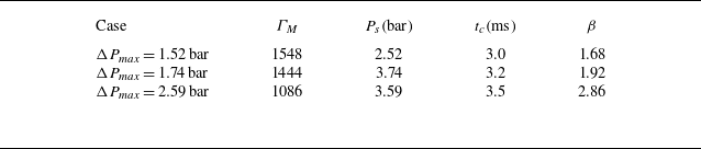
In the further model assessment, figure 13 shows that the model estimation in (4.20) generally agrees with the experimental results (Xue et al. Reference Xue, Du, Shi, Gan and Bai2018). The parameters used in the comparison between the model estimation in (4.20) and the experimental results are listed in table 2. The critical time $t_c$ is extracted from the experimental data because (4.8) does not hold for the initially loose-packed particle bed ( $\varPhi _0=0.39$ ) in the experiments. Experimental cases with different pressure histories are fitted with distinct values of $\beta$ . Stronger blast waves (larger max overpressure ( $\Delta P_{\textit{max}}$ )) compress the particle bed more tightly, resulting in a smaller $h_c$ . Thus, a larger $\beta$ is required to correct the overestimated $h_c$ in the model (see Appendix D for details). The fitting parameter $\beta =1.68$ in the case with $\Delta P_{\textit{max}}=1.52\,\mathrm{bar}$ is determined by minimising the mean-squared error between experimental data and model predictions. Subsequent linear fitting yields the relationship $\beta =1.105\Delta P_{\textit{max}}/P_0$ , from which the values for cases with $\Delta P_{\textit{max}}=1.74\,\mathrm{bar}$ and $\Delta P_{\textit{max}}=2.59\,\mathrm{bar}$ are calculated as $\beta = 1.92$ and $2.86$ , respectively. Moreover, the model slightly overestimates $L_{\textit{jr}}$ at the late stage. This is because the external surface is penetrated, and then the magnitude of $a_c$ is overestimated in (4.16).

Table 2.

Summary of the parameters used in our model (4.20) for the experimental cases in Xue et al. (Reference Xue, Du, Shi, Gan and Bai2018). Note that $L_{\textit{jr}}(t_{c})=0\,\mathrm{mm}$ , $R_{I0}=10\,\mathrm{mm}$ , $h=20\,\mathrm{mm}$ and $\varPhi _{0}=0.39$ are used in modelling all the experimental cases. Since the experiments are in a three-dimensional configuration, the volume fraction of the compacted particle bed is set to $\varPhi _{\textit{comp}}=0.65$ for modelling all the experimental cases.

Therefore, the RTI, RMI and large particle inertia lead to the external particle jet formation. The morphological evolution of the dispersed particle bed is dominated by three particle-loosening events: internal particle shedding, external particle jetting and bidirectional particle fingering (Xue et al. Reference Xue, Miu, Li, Bai and Tian2023). For large $P_{s}$ or small $h$ , the internal particle shedding dominates the dispersal process. For large $h$ , the bidirectional particle fingering dominates the dispersal process. For small $P_{s}$ , the external particle jet does not occur due to the large particle inertia.