Sterba and Bauer conclude that dynamic factor analysis does not enable testing of two of the six person-oriented principles, namely, the complex interactions principle and the interindividual differences/intraindividual change principle. In this section I will show that this conclusion no longer holds in view of recent developments in dynamic factor modeling. Hence, I will conclude that dynamic factor analysis in its present form enables testing of all six person-oriented principles considered by Sterba and Bauer.
The dynamic factor model in its present form
It will be helpful to specify in schematic form the dynamic factor model in its present form. In doing so several details will not be considered and only a simplified form of the model will be presented. The all-important issue of the ways in which the model can be fitted to the data will not be considered.
The main simplifications of the model scheme to be presented involve the following three caveats. (a) The model scheme lacks lagged factor loadings. It only allows for contemporaneous relationships between the observed multivariate series and the latent factor process. Adding lagged relationships between the observed multivariate series and the latent factor process, as in the original dynamic factor model introduced in Molenaar (Reference Molenaar1985), would not affect the main arguments to be presented below, and therefore are omitted to ease the presentation. (b) The model scheme does not involve explicit notation to indicate that it is applicable to multiple subjects. This is omitted to ease the presentation of the model scheme itself, because it would imply adding person-specific superscripts to all model parameters. It will be understood that the model scheme to be presented can be applied to multivariate time series obtained with multiple subjects in a replicated time series design. (c) The model scheme does not represent mean time-dependent trends. These can be added straightforwardly without affecting the main arguments to be presented below.
Let y(t) denote a p-variate observed time series, where time t is proceeding in discrete steps: t = 1, 2, … T. For instance, y(t) represents daily measurements of p disease symptoms. In addition, let η(t) denote a q-variate latent factor process; q < p. For instance, for q = 1 the latent factor series represents the univariate disease process underlying the observed symptoms. Here, u(t) denotes an r-dimensional time-varying covariate (external input). For instance, for r = 1, the external input involves daily registrations of medication dose. Finally, all unknown model parameters (e.g., factor loadings) are collected in a vector θt. Notice that the vector θt of unknown model parameters is itself allowed to vary in time. Moreover, it is important that the way in which the model parameters vary in time is assumed to be unknown as well. With these definitions, the dynamic factor model in its current form can be schematically represented as
Expression 1a is a factor model in which the observed time series y(t) is regressed upon the latent factor process η(t). The (p, q)-dimensional matrix Λ[θt] contains the factor loadings that, as elements of the parameter vector θt, are allowed to vary in time in arbitrary ways; and ɛ(t) is the p-variate measurement error process. Expression 1b is a vector regression model in which the factor process at time t + 1, η(t + 1), is regressed upon itself at the previous time t. Hence, Equation 1b is often called a vector autoregression model; B[θt] is the (q, q)-dimensional matrix of (auto)regression coefficients of η(t + 1) on η(t). It is associated with the stability of the latent factor process. Each unknown regression coefficient in B[θt] is an element of the parameter vector θt, and therefore is allowed to vary in time in arbitrary ways, and Γ[θt] is a (q, r)-dimensional matrix of regression coefficients quantifying the effects of the external input u(t) on the factor process. Each unknown regression coefficient in Γ[θt] is an element of the parameter vector θt, and therefore is allowed to vary in time in arbitrary ways. Finally, ζ(t) is q-variate process noise.
The statistical tools to fit extended dynamic factor models expressed by Equation 1 have become available only recently (Molenaar, Sinclair, Rovine, Ram, & Corneal, Reference Molenaar, Sinclair, Rovine, Ram and Corneal2009). Allowing the vector θt of unknown parameters to vary in time in arbitrary ways heavily complicates the way in which the model is fitted to the data. Until now, almost all variants of dynamic factor models are fitted to the data under the assumption that all unknown parameters are constant in time: θt = θ for all t. To the best of my knowledge, the only exceptions are considered in Molenaar, de Gooijer, and Schmitz (Reference Molenaar, de Gooijer and Schmitz1992) and Molenaar (Reference Molenaar, Von Eye and Clogg1994). Model 1 is based on Molenaar and Newell (Reference Molenaar and Newell2003) and constitutes a fundamental extension of these earlier analogues.
A final important remark about Equation 1 should be made. Model parameters in Equation 1 are allowed to vary in time in arbitrary ways. This implies that no parametric representation of the ways in which model parameters change in time is required. For instance, no assumptions that these model parameters change linearly, or exponentially, or logarithmically, or according to any other functional form, are required. The only soft assumption made to enable estimation of the time-varying model parameters in Equation 1 is that these parameters are slowly changing in comparison to the changes in the observed time series y(t). A useful mathematical criterion for “slowly changing” is given by Priestley (Reference Priestley1988). Of course, after the slowly time-varying parameters in Equation 1 have been estimated, one always has the option to fit a posteriori suitable parametric forms to their time-dependent trajectories by means of the method introduced in Molenaar (Reference Molenaar, Von Eye and Clogg1994).
Testing the interindividual differences/intraindividual change principle by means of dynamic factor analysis
Sterba and Bauer conclude that the interindividual differences/intraindividual change principle is difficult to assess using the standard dynamic factor analysis model because this model assumes no systematic intraindividual change, growth, or development in means, variances, or covariances of measured variables. This conclusion is correct: the standard dynamic factor model introduced in Molenaar (Reference Molenaar1985) is based on the assumption that model parameters do not vary in time. However, in the dynamic factor model in its present form this restrictive assumption is no longer being made. In the extended dynamic factor model expressed by Equation 1 all model parameters are allowed to be time varying in arbitrary ways. Consequently, the interindividual differences/intraindividual change principle can be assessed using Equation 1.
It was indicated above that Equation 1 represents a simplified model scheme of the extended dynamic factor model in its current form. Time-varying mean trends can be straightforwardly accommodated by the model in several distinct ways. For instance, a vector of time-varying means can be added to Equaton 1a or 1b, where these means constitute additional unknown parameters that are added to the parameter vector θt. To accommodate time-varying variances and covariances of the measurement error process ɛ(t) and/or the process noise ζ(t) requires more ingenuity. This is investigated in an ongoing research project, the initial results of which are promising and will be reported in a forthcoming publication. It is noted that an alternative class of dynamic models accommodating time-varying variances and covariances is prominent in the econometrics literature (so-called multivariate autoregressive conditionally heteroskedastic models; cf. Lütkepohl, Reference Lütkepohl2005, pp. 562–582).
Testing the complex interactions principle by means of dynamic factor analysis
The complex interactions principle concerns Person × Context × Time interactions. Sterba and Bauer conclude that assessment of the complex interactions principle by means of dynamic factor analysis is impossible. The reasons they give for this conclusion are the following: “In a dynamic factor analysis . . . for a single person, incorporating time-invariant person, or context, or person × context predictors of process factors would not be helpful because they would just be constant values for that one person; and incorporating time-variant person, or context, or person × context predictors of process factors would only be useful for explaining interoccasion variability.” Their conclusion is correct, but it is based on an unnecessary restricted variant of dynamic factor analysis. In the following I will neglect their appeal to time-invariant predictors, because the dynamic factor Model 1 can handle time-varying covariates (external input, predictors). If no time-varying covariates are available, then this is not the fault of the dynamic factor model.
The unnecessary restriction, which is of importance because it gives rise to Sterba and Bauer's conclusion that assessment of the complex interactions principle by means dynamic factor analysis is impossible, is the following. They restrict application of the dynamic factor model to single subjects. However, as indicated above, the extended dynamic factor Model 1 can be applied to multivariate time series obtained with multiple subjects in a replicated time series design. Given that we have multiple subjects, instances of Equation 1 can be simultaneously fitted to the multivariate time series of each subject in a manner that is akin to multigroup analysis in standard structural equation modeling of interindividual variation. It then is possible to test for equalities across subjects of arbitrary subsets of model parameters by means of likelihood ratio tests. If such equalities cannot be rejected for particular subsets of model parameters, then this implies that the implied interactions are not significant. Adding different contexts can be accomplished by adding appropriate indicators to the external input u(t) in Equation 1. Tests of complex interactions involving contexts then will focus on the lack of equality across subjects of parameters in Γ[θt].
To the best of my knowledge, no published applications of tests of the complex interaction principle using the dynamic factor Model 1 are presently available. Yet, the approach to test for Person × Context × Time interactions sketched above shows that such assessments are feasible. Other feasible approaches are possible, however. For instance, suppose that the unit of analysis in dynamic factor analysis is not the subject, but a group (e.g., client–therapist dyad, mother–child dyad, nuclear family, etc.). The component series in the observed multivariate time series y(t) now constitute contemporaneous measurements of each group member. Tests of interactions involving persons based on Equation 1 then will focus on the lack equality of parameters in B[θt] across different contexts. Without doubt, other feasible approaches are possible. This is a methodological issue that is as yet unexplored.





 You have
Access
Sterba and Bauer's Keynote Article presents a revealing comparison of person-oriented methods to test person-oriented theoretical principles in developmental psychopathology research. Their thorough assessment of the strengths and weaknesses of person-oriented methods, summarized in table 2 of their Keynote, constitutes an eminent contribution to person-oriented research.
In this Commentary I will focus on one of the methods assessed by Sterba and Bauer: single-subject methods such as dynamic factor analysis of multivariate time series. In their assessment of single-subject methods Sterba and Bauer conclude that dynamic factor analysis is able to test four person-oriented principles, but it has difficulty handling the other two. The person-oriented principles that dynamic factor analysis is able to test are individual specificity (of statistical models), pattern summary (of multivariate variables), holism (reduction of multivariate variables to component variables), and pattern parsimony (reduction to limited number of component variables). The person-oriented principles that are considered to be difficult or impossible to test with dynamic factor analysis are complex (e.g., Person × Context × Time) interactions and interindividual differences/intraindividual change. It will be shown that recent extensions of the dynamic factor model enable testing the latter two person-oriented as well. This implies that, in its current form, dynamic factor analysis can test all six person-oriented principles in developmental psychopathology research.
Dynamic factor analysis has recently been extended in ways that transcend its capability to test the six person-oriented principles in developmental psychopathology research in important ways. Dynamic factor analysis is based on a general dynamic systems model that explains the time-dependent evolution of multivariate observed processes in terms of a limited number of latent factor processes. The evolution of a latent factor process itself can be modeled as being influenced by time-varying covariates, where these covariates can be conceived of as measured external input to the dynamic systems model. For instance, if the latent factor process denotes a disease process, then the time-varying covariates (external input) affecting this disease process could be observed time series of changing environmental conditions, therapeutic manipulations, medication dose, and so forth. This extension of the dynamic factor model with time-varying external input affecting the evolution of the latent factor process opens up the possibility to optimally steer the factor process to desired levels. This is accomplished by applying optimal control theory to the extended dynamic factor model, a powerful technique used in computational engineering. In this way the values of external input are determined at each point in time so that the latent factor process is optimally steered to desired levels. For instance, if the latent factor process denotes a disease process and external input is medication dose, then at each point in time the time-varying dose of medication can be determined so that the disease process is optimally treated. An empirical illustration of this will be presented in what follows. To start with, however, some preliminary issues have to be addressed.
Preliminary Issues
In this section the important distinctions between interindividual and intraindividual variation and between person-oriented and person-specific methods are defined. A straightforward extension of the definition of single-subject methods is also introduced.
Inter- versus intraindividual variation
All person-oriented methods discussed by Sterba and Bauer, except one, are methods for the analysis of interindividual variation, which is the variation between individuals. Only the single-subject method is a method for the analysis of intraindividual variation, which is the variation within an individual. As is noted by Sterba and Bauer, analysis of interindividual variation is the standard approach in psychology. Its defining features are the following: (a) a random sample of subjects is drawn from a given population; (b) it is assumed that the population of subjects is homogeneous, that is, subjects are exchangeable and all obey the same statistical model; (c) statistics of interest are estimated by pooling across the sampled subjects; and (d) the results of statistical analysis usually are generalized to the population of subjects from which the random sample was drawn. This definition of analysis of interindividual variation can be straightforwardly refined for mixture analysis. In contrast, the defining features of analysis of intraindividual variation are (a) a given subject is repeatedly measured during an interval of time, where this interval of time is considered to be a block of time points randomly drawn from the entire time axis; (b) statistics of interest are estimated by pooling across time points; and (c) the results of statistical analysis are generalized along the entire time axis (retrodiction, interpolation, prediction).
It is an implicit assumption of methods for the analysis of interindividual variation that the results thus obtained also apply at the level of intraindividual variation. For instance, most psychological inventories are constructed by means of classical test theory using factor analysis of interindividual variation (Lord & Novick, Reference Lord and Novick1968). An important application of many of these inventories is in individual assessment and prediction, that is, applications at the level of intraindividual variation of individual subjects. It then is assumed that the reliabilities and validities of these inventories, as assessed in factor analyses of interindividual variation, also are valid for individual assessment of intraindividual variation. However, Molenaar (Reference Molenaar, Hofer and Alwin2008) shows that this assumption is invalid (see also Borsboom, Reference Borsboom2005) and that individual assessments and predictions thus obtained can be seriously erred even if nominal reliabilities and validities are high. The reason is that the statistical model underlying classical test theory violates a fundamental mathematical theorem stipulating the conditions that must obeyed so that results obtained in analyses of interindividual variation can be validly generalized to intraindividual variation and vice versa. This theorem is called the individual ergodic theorem, and its profound consequences for the analysis of psychological processes are explained in Molenaar (Reference Molenaar2004). In particular, all learning and developmental processes violate the conditions stipulated by the individual ergodic theorem, and therefore their analysis should be based on intraindividual variation, not interindividual variation (cf. Molenaar, Reference Molenaar2007). Hence, for all learning and developmental processes, including all processes having time-varying statistical characteristics, it is not an option but a necessity to base their analysis on intraindividual variation.
Person-oriented versus person-specific methods
Sterba and Bauer present an excellent overview of person-oriented methods, one of which is referred to as single-subject methods. As indicated above, only single-subject methods, in particular dynamic factor analysis, are methods for the analysis of intraindividual variation, whereas the remaining methods discussed by Sterba and Bauer are methods for the analysis of interindividual variation. However, methods for the analysis of intraindividual variation, the importance of which is implied by the individual ergodic theorem, are commonly referred to as person-specific methods (Molenaar & Campbell, Reference Molenaar and Campbell2009). As will be argued below, person-specific methods are excellently equipped to test all person-oriented principles specified by Sterba and Bauer. However, the essence of person-specific methods is that they are methods for the analysis of intraindividual variation; their application in tests of person-oriented principles is, although important in itself, secondary.
Single-subject versus person-specific methods
Sterba and Bauer refer to dynamic factor analysis as a single-subject method. This, or its synonym single-case method, is a common denotation for methods like dynamic factor analysis (e.g., Barlow, Nock, & Hersen, Reference Barlow, Nock and Hersen2009). Unfortunately, it then is incorrectly suggested that dynamic factor analysis is restricted to single-subject time series. This is not the case: dynamic factor analysis can be (and has been; cf. Hamaker, Dolan, & Molenaar, Reference Hamaker, Dolan and Molenaar2005) applied to multivariate time series obtained with multiple subjects in a replicated time series design. This enables precise testing of commonalities across subjects. It thus may be found by means of most powerful likelihood ratio tests that particular subsets of subjects share the same factor loadings for some (or all) of the latent factor processes and/or have the same values for other model parameters. In particular, it thus can be tested whether all or a subset of subjects obey the new definition of measurement equivalence proposed by Nesselroade, Gerstorf, Hardy, and Ram (Reference Nesselroade, Gerstorf, Hardy and Ram2007). In what follows I therefore will refer to dynamic factor analysis as a person-specific method.
Dynamic Factor Analysis Enables Complete Testing of Person-Oriented Principles
Sterba and Bauer conclude that dynamic factor analysis does not enable testing of two of the six person-oriented principles, namely, the complex interactions principle and the interindividual differences/intraindividual change principle. In this section I will show that this conclusion no longer holds in view of recent developments in dynamic factor modeling. Hence, I will conclude that dynamic factor analysis in its present form enables testing of all six person-oriented principles considered by Sterba and Bauer.
The dynamic factor model in its present form
It will be helpful to specify in schematic form the dynamic factor model in its present form. In doing so several details will not be considered and only a simplified form of the model will be presented. The all-important issue of the ways in which the model can be fitted to the data will not be considered.
The main simplifications of the model scheme to be presented involve the following three caveats. (a) The model scheme lacks lagged factor loadings. It only allows for contemporaneous relationships between the observed multivariate series and the latent factor process. Adding lagged relationships between the observed multivariate series and the latent factor process, as in the original dynamic factor model introduced in Molenaar (Reference Molenaar1985), would not affect the main arguments to be presented below, and therefore are omitted to ease the presentation. (b) The model scheme does not involve explicit notation to indicate that it is applicable to multiple subjects. This is omitted to ease the presentation of the model scheme itself, because it would imply adding person-specific superscripts to all model parameters. It will be understood that the model scheme to be presented can be applied to multivariate time series obtained with multiple subjects in a replicated time series design. (c) The model scheme does not represent mean time-dependent trends. These can be added straightforwardly without affecting the main arguments to be presented below.
Let y(t) denote a p-variate observed time series, where time t is proceeding in discrete steps: t = 1, 2, … T. For instance, y(t) represents daily measurements of p disease symptoms. In addition, let η(t) denote a q-variate latent factor process; q < p. For instance, for q = 1 the latent factor series represents the univariate disease process underlying the observed symptoms. Here, u(t) denotes an r-dimensional time-varying covariate (external input). For instance, for r = 1, the external input involves daily registrations of medication dose. Finally, all unknown model parameters (e.g., factor loadings) are collected in a vector θt. Notice that the vector θt of unknown model parameters is itself allowed to vary in time. Moreover, it is important that the way in which the model parameters vary in time is assumed to be unknown as well. With these definitions, the dynamic factor model in its current form can be schematically represented as
Expression 1a is a factor model in which the observed time series y(t) is regressed upon the latent factor process η(t). The (p, q)-dimensional matrix Λ[θt] contains the factor loadings that, as elements of the parameter vector θt, are allowed to vary in time in arbitrary ways; and ɛ(t) is the p-variate measurement error process. Expression 1b is a vector regression model in which the factor process at time t + 1, η(t + 1), is regressed upon itself at the previous time t. Hence, Equation 1b is often called a vector autoregression model; B[θt] is the (q, q)-dimensional matrix of (auto)regression coefficients of η(t + 1) on η(t). It is associated with the stability of the latent factor process. Each unknown regression coefficient in B[θt] is an element of the parameter vector θt, and therefore is allowed to vary in time in arbitrary ways, and Γ[θt] is a (q, r)-dimensional matrix of regression coefficients quantifying the effects of the external input u(t) on the factor process. Each unknown regression coefficient in Γ[θt] is an element of the parameter vector θt, and therefore is allowed to vary in time in arbitrary ways. Finally, ζ(t) is q-variate process noise.
The statistical tools to fit extended dynamic factor models expressed by Equation 1 have become available only recently (Molenaar, Sinclair, Rovine, Ram, & Corneal, Reference Molenaar, Sinclair, Rovine, Ram and Corneal2009). Allowing the vector θt of unknown parameters to vary in time in arbitrary ways heavily complicates the way in which the model is fitted to the data. Until now, almost all variants of dynamic factor models are fitted to the data under the assumption that all unknown parameters are constant in time: θt = θ for all t. To the best of my knowledge, the only exceptions are considered in Molenaar, de Gooijer, and Schmitz (Reference Molenaar, de Gooijer and Schmitz1992) and Molenaar (Reference Molenaar, Von Eye and Clogg1994). Model 1 is based on Molenaar and Newell (Reference Molenaar and Newell2003) and constitutes a fundamental extension of these earlier analogues.
A final important remark about Equation 1 should be made. Model parameters in Equation 1 are allowed to vary in time in arbitrary ways. This implies that no parametric representation of the ways in which model parameters change in time is required. For instance, no assumptions that these model parameters change linearly, or exponentially, or logarithmically, or according to any other functional form, are required. The only soft assumption made to enable estimation of the time-varying model parameters in Equation 1 is that these parameters are slowly changing in comparison to the changes in the observed time series y(t). A useful mathematical criterion for “slowly changing” is given by Priestley (Reference Priestley1988). Of course, after the slowly time-varying parameters in Equation 1 have been estimated, one always has the option to fit a posteriori suitable parametric forms to their time-dependent trajectories by means of the method introduced in Molenaar (Reference Molenaar, Von Eye and Clogg1994).
Testing the interindividual differences/intraindividual change principle by means of dynamic factor analysis
Sterba and Bauer conclude that the interindividual differences/intraindividual change principle is difficult to assess using the standard dynamic factor analysis model because this model assumes no systematic intraindividual change, growth, or development in means, variances, or covariances of measured variables. This conclusion is correct: the standard dynamic factor model introduced in Molenaar (Reference Molenaar1985) is based on the assumption that model parameters do not vary in time. However, in the dynamic factor model in its present form this restrictive assumption is no longer being made. In the extended dynamic factor model expressed by Equation 1 all model parameters are allowed to be time varying in arbitrary ways. Consequently, the interindividual differences/intraindividual change principle can be assessed using Equation 1.
It was indicated above that Equation 1 represents a simplified model scheme of the extended dynamic factor model in its current form. Time-varying mean trends can be straightforwardly accommodated by the model in several distinct ways. For instance, a vector of time-varying means can be added to Equaton 1a or 1b, where these means constitute additional unknown parameters that are added to the parameter vector θt. To accommodate time-varying variances and covariances of the measurement error process ɛ(t) and/or the process noise ζ(t) requires more ingenuity. This is investigated in an ongoing research project, the initial results of which are promising and will be reported in a forthcoming publication. It is noted that an alternative class of dynamic models accommodating time-varying variances and covariances is prominent in the econometrics literature (so-called multivariate autoregressive conditionally heteroskedastic models; cf. Lütkepohl, Reference Lütkepohl2005, pp. 562–582).
Testing the complex interactions principle by means of dynamic factor analysis
The complex interactions principle concerns Person × Context × Time interactions. Sterba and Bauer conclude that assessment of the complex interactions principle by means of dynamic factor analysis is impossible. The reasons they give for this conclusion are the following: “In a dynamic factor analysis . . . for a single person, incorporating time-invariant person, or context, or person × context predictors of process factors would not be helpful because they would just be constant values for that one person; and incorporating time-variant person, or context, or person × context predictors of process factors would only be useful for explaining interoccasion variability.” Their conclusion is correct, but it is based on an unnecessary restricted variant of dynamic factor analysis. In the following I will neglect their appeal to time-invariant predictors, because the dynamic factor Model 1 can handle time-varying covariates (external input, predictors). If no time-varying covariates are available, then this is not the fault of the dynamic factor model.
The unnecessary restriction, which is of importance because it gives rise to Sterba and Bauer's conclusion that assessment of the complex interactions principle by means dynamic factor analysis is impossible, is the following. They restrict application of the dynamic factor model to single subjects. However, as indicated above, the extended dynamic factor Model 1 can be applied to multivariate time series obtained with multiple subjects in a replicated time series design. Given that we have multiple subjects, instances of Equation 1 can be simultaneously fitted to the multivariate time series of each subject in a manner that is akin to multigroup analysis in standard structural equation modeling of interindividual variation. It then is possible to test for equalities across subjects of arbitrary subsets of model parameters by means of likelihood ratio tests. If such equalities cannot be rejected for particular subsets of model parameters, then this implies that the implied interactions are not significant. Adding different contexts can be accomplished by adding appropriate indicators to the external input u(t) in Equation 1. Tests of complex interactions involving contexts then will focus on the lack of equality across subjects of parameters in Γ[θt].
To the best of my knowledge, no published applications of tests of the complex interaction principle using the dynamic factor Model 1 are presently available. Yet, the approach to test for Person × Context × Time interactions sketched above shows that such assessments are feasible. Other feasible approaches are possible, however. For instance, suppose that the unit of analysis in dynamic factor analysis is not the subject, but a group (e.g., client–therapist dyad, mother–child dyad, nuclear family, etc.). The component series in the observed multivariate time series y(t) now constitute contemporaneous measurements of each group member. Tests of interactions involving persons based on Equation 1 then will focus on the lack equality of parameters in B[θt] across different contexts. Without doubt, other feasible approaches are possible. This is a methodological issue that is as yet unexplored.
Optimal Control of Developmental Psychopathological Processes
For quite a long time there has been continuing interest of theoretical psychologists in control theory. More recent publications apply control theory for instance to depression (Hyland, Reference Hyland1987), self-regulation of behavior (Carver & Scheier, Reference Carver and Scheier1998), and cognition and behavior (Johnson, Chang, & Lord, Reference Johnson, Chang and Lord2006). As these applications demonstrate, control models have always been considered in a theoretical context. To the best of our knowledge, control theory has never been used as a computational tool to actually optimize developmental and learning processes. In the following a schematic description is provided of the use of control theory to steer developmental processes to desired levels and keep them there. A concise illustration to optimal patient-specific control of a disease process is given at the close of this section.
Suppose that Equation 1 provides a faithful description of the p-variate time series y(t). Suppose also that the external input u(t) consists of variables that can be manipulated by the controller (e.g., therapist). It then is possible to determine at each time t the optimal external input u(t) in such a way that the state process (e.g., disease process) η(t) is steered to its desired level η#, where η# is chosen by the controller. In terms of Equation 1, the optimal input uopt(t) is determined according to the following schematic feedback function:
where Ft(·) denotes an (r, p)-dimensional time-varying feedback function. Application of uopt(t) at each time t guarantees that the state process η(t + 1) at the next time point t + 1 will be as close as possible to the desired level η#. Derivation of the mathematical form of the feedback function Ft(·) is given in Molenaar (Reference Molenaar and Campbell2009).
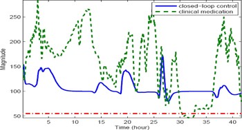
To illustrate the power of feedback control, an application to optimal patient-specific control of a disease process is given. Because at present empirical applications to psychopathological processes are still lacking, the application of Equations 1 and 2 to diabetic type 1 patients is considered (for details, see Molenaar, Ulbrecht, et al., Reference Molenaar, Ulbrecht, Gold, Rovine, Wang and Zhou2009). Here, y(t) is the observed blood glucose level of a single patient, continuously measured at 5-min intervals during about 41 hr. The measured external input u(t) consists of insulin dose and meal intake (carbohydrates). A particular instance of the dynamic factor Model 1 was fitted to the data of this patient. Then, based on the estimates of the time-varying parameters θt at each time t, the optimal insulin dose was determined according to Equation 2, using η# = 100 as the desired blood glucose level. These optimal values of insulin dose were not actually administered (this will be done in a follow-up study), but instead, the patient applied the clinically prescribed insulin doses. The broken line in Figure 1 depicts the actual fluctuations of the patient's blood glucose level using this clinical medication. It is apparent that the fluctuations substantially deviate from the desired level of η# = 100. The continuous line shows the expected blood glucose concentrations that would have occurred if the patient would have used the time-varying optimal insulin dose. The lower constant line indicates a blood glucose level of 60, which is considered immediately dangerous. It is apparent that the optimal insulin dose would have substantially reduced the deviations of blood glucose from its desired level of η# = 100. Similar subject-specific applications of computational control theory based on the dynamic factor model can be envisioned regarding the optimization of psychotherapeutic processes (Molenaar, in press), learning processes, and developmental processes in general.
The magnitude versus time for the administration of clinical medication. [A color version of this figure can be viewed online at journals.cambridge.org/dpp]