


A psychological measure does not exist in a situational vacuum (Anastasi, Reference Anastasi, Wainer and Messick1983; Steyer, Mayer, Geiser, & Cole, Reference Steyer, Mayer, Geiser and Cole2015). Psychological assessments made at a given point in time, as in a cross-sectional study, cannot disentangle the enduring characteristics of a person from those of that person in that specific situation. Longitudinal studies allow better understanding of whether changes in observed psychometric scores over repeated measurements reflect changes in stable psychological attributes (e.g. traits), situational fluctuations (i.e. occasion-specific effects), method effects, or measurement error (Geiser & Lockhart, Reference Geiser and Lockhart2012; Steyer et al., Reference Steyer, Mayer, Geiser and Cole2015). Although classical longitudinal analytical approaches such as repeated measures analysis of variance/covariance assess both within- and between-subject variances, they do not explicitly disentangle situational or ‘state’ fluctuations v. relatively stable ‘trait’ sources of information (Curran, Howard, Bainter, Lane, & Mcginley, Reference Curran, Howard, Bainter, Lane and Mcginley2014; Mehl & Conner, Reference Mehl and Conner2012). Latent state-trait (LST) models have been proposed (Schmitt & Steyer, Reference Schmitt and Steyer1993; Steyer, Reference Steyer1988; Steyer et al., Reference Steyer, Mayer, Geiser and Cole2015; Steyer, Ferring, & Schmitt, Reference Steyer, Ferring and Schmitt1992; Steyer, Majcen, Schwenkmezger, & Buchner, Reference Steyer, Majcen, Schwenkmezger and Buchner1989; Steyer, Schmitt, & Eid, Reference Steyer, Schmitt and Eid1999; revised in Steyer et al., Reference Steyer, Mayer, Geiser and Cole2015) to decompose measurements into these two main sources of information as latent random variables in the context of confirmatory factor analysis (Steyer et al., Reference Steyer, Mayer, Geiser and Cole2015) (see Steyer et al., Reference Steyer, Ferring and Schmitt1992). The idea of disentangling behaviors in terms of state and trait was posed even before the LST theory, statistically formalized by Rolf Steyer, by the work of Netherlands Psychologist Johan Ormel titled Neuroticism and well-being inventories: Measuring traits or states? (Ormel, Reference Ormel1983).
Recently, Eid, Holtmann, Santangelo, and Ebner-Priemer (Reference Eid, Holtmann, Santangelo and Ebner-Priemer2017), based on the revision of LST theory (LST-R theory) of Steyer et al. (Reference Steyer, Mayer, Geiser and Cole2015), extended the model called trait-state-occasion (TSO) proposed by Cole, Martin, and Steiger (Reference Cole, Martin and Steiger2005), which is one of the most popular LST models (Prenoveau, Reference Prenoveau2016). In LST-R theory, an observed variable is decomposed into three components: a trait component, an occasion-specific component representing influences due to the situation and/or situation–person interaction, and a measurement error variable (Steyer et al., Reference Steyer, Mayer, Geiser and Cole2015). The trait is considered a disposition of an individual at a time of measurement t. That means that traits can change over time, even within short time periods. Moreover, situational experiences can lead to trait change. Eid et al. (Reference Eid, Holtmann, Santangelo and Ebner-Priemer2017) defined a LST model with autoregressive effects that explicitly models this idea. In this model, the disposition to react to specific situations on an occasion of measurement t can depend on a situational experience on the occasion of measurement before (t − 1). For example, being informed about an unexpected substantial salary increase might not only increase the positive mood on that occasion of measurement but might also result in a changed disposition to react to daily hassles 2 hours later – the person might react less negatively to a daily hassle (like missing a bus). LST-R theory considers personality as a dynamic system (not a fixed entity) that reacts to and changes according to environmental influences. If traits can change according to situational influences psychometric models have to consider these dynamic views. If situational influence changes traits, situational influences can accumulate over time. Eid et al.'s (Reference Eid, Holtmann, Santangelo and Ebner-Priemer2017) approach represents this basic idea of psychological constructs (i.e. personality and psychopathology) as a dynamic system. According to their model individual trait differences on an occasion of measurement depends on the trait on the first occasion of measurement (when the process starts) and accumulated situational experiences (accumulated life experiences). That means that dispositional differences represent initial trait differences as well as individual differences in what happens in one's life. If one considers, for example, a longitudinal study on depression with annual measurements over five years the disposition to depressive mood might depend on the depression trait on the first occasion of measurement but also on how enjoyable or frustrating life experiences were between. It is not very likely that the disposition to react to situational stimuli is stable over such a long time period. There are dispositions to react to situations with depressive mood on each occasion of measurement. However, they might not be totally stable over time. Because situations can change traits in such a dynamic conception of personality, situational effects can accumulate over time. For example, if a person experiences many enjoyable life events over a time period the effects of these positive life events can cumulate over time. As Eid et al. (Reference Eid, Holtmann, Santangelo and Ebner-Priemer2017) have shown, a LST-R model with autoregressive effects represents this basic idea. In such a model individual trait differences on an occasion of measurement can be decomposed into differences that are predictable by trait differences on the first occasion of measurement (trait stability) and by accumulated situational effects (life experiences). Like in every latent state trait model an observed variable on an occasion of measurement can be decomposed into individual trait differences (consistency), occasion-specific differences (occasion specificity) and measurement error (unreliability), but the consistency coefficient can be further decomposed into one part indicating stability due to trait stability (predictability by the trait on the occasion of measurement when the process started) and stability due to effects of situations (life events) over time. It is important to note that the situations and life events do not have to be explicitly measured but their influence can be modeled within the measurement model considered (Steyer et al., Reference Steyer, Mayer, Geiser and Cole2015). The decomposition of the consistency coefficient into two parts representing stability due to trait and due to accumulated situational effects over time is particularly important for clinical assessment as it allows a better understanding of stability and change processes. It also has implications for the study of age, period and cohort effects as trait effects over time can be thought of as the result of cohort effects and/or the aging process, whereas occasion specific differences represent period effects (Keyes et al., Reference Keyes, Nicholson, Kinley, Raposo, Stein, Goldner and Sareen2014).
Using the approach described above, it is also possible to examine whether psychological symptoms capture equally trait and state information between sexes groups and whether there are sex differences in how previous experiences influence trait change over time. This is particularly important because longitudinal studies describe a higher frequency of psychological symptoms in women, that is relatively stable over time, suggesting that symptoms are more a trait-like phenomenon for women than for men (Furnham & Cheng, Reference Furnham and Cheng2015). However, no study has yet separated occasion-specific components as well as trait and accumulated situational effects on psychological distress over time. These components might differ between the sexes for a number of psychosocial and biological reasons (de Kruif, Spijker, & Molendijk, Reference de Kruif, Spijker and Molendijk2016; Maeng & Milad, Reference Maeng and Milad2015). It has been suggested that in women, increased vulnerability emerges at age 13–15 (Salk, Hyde, & Abramson, Reference Salk, Hyde and Abramson2017), but this may decrease with aging (Kessler et al., Reference Kessler, Birnbaum, Bromet, Hwang, Sampson and Shahly2010).
Using the latent-state-trait model with autoregressive effects (LST-AR) specified by Eid et al. (Reference Eid, Holtmann, Santangelo and Ebner-Priemer2017), we aimed to determine the consistency (trait differences and accumulated effects) and occasion specificity of psychological distress symptoms in men and women throughout adult life. We use the nine dichotomous indicators of the Malaise Inventory (e.g. depressed mood, worry, anger, nervousness, agitation, etc.) that represent important symptoms related to psychological distress (Rodgers, Pickles, Power, Collishaw, & Maughan, Reference Rodgers, Pickles, Power, Collishaw and Maughan1999), measured in four waves from young adulthood to middle age, in two different British birth cohorts, to disentangle the relative consistency and occasion specificity in male and females.
Although differences between males and females in terms of psychological distress are classically reported (Salk et al., Reference Salk, Hyde and Abramson2017), these studies did not separate between- and within-group variance, which might lead to wrong conclusions about either (or both); moreover, each symptom might measure traits and states differently. Another important feature observable under the LST-AR model, in contrast to previous models such as that proposed by Cole et al. (Reference Cole, Martin and Steiger2005), is the stability of the constructs over time. Taking these considerations into account, the current study sought to determine if the predisposition to, state fluctuations in, and previous experiences of psychological distress might be perceived equally between males and females, and if these effects were consistent across two different historical moments.
Methods
Cohorts
In this study we used data from two British birth cohort surveys: the National Child Development Study (NCDS58), also known as the 1958 Birth Study, and the 1970 cohort, called the 1970 British Cohort Study (BCS70). Both followed groups of people from birth through adulthood, adopting a sequential mixed-model design. Over the years, information has been gathered from a number of sources (e.g. parents, health service personnel, and the cohort members themselves) and in a variety of ways (e.g. face-to-face and telephone interviews, self-completion paper posted/given and electronic questionnaires, and medical records). Most of the sweeps were carried out face-to face with interview conducted by nurses in the cohort members' homes (TNS BMRB, 2014). Both cohorts are managed by the Centre for Longitudinal Studies (CLS) and funded by the Economic and Social research Council.
The National Child Development Study (NCDS58), which started as the Perinatal Mortality Survey (PMS), is a birth cohort of over 17 638 births (live or dead) in England, Scotland, and Wales, as well as the Channel Islands, Isle of Man, and other offshore islands, from over a single week, 3–9 March 1958 (TNS BMRB, 2013, 2014). The current study selected waves 4 (NCDS4) at age 23 (1981), 5 (NCDS5) at age 33 (1991), 6 (NCDS6) at age 42 (2000), and 8 (NCDS8) at age 50 (2008).
Nine waves of data were collected from birth (1958) to the age of 55 (2013). Survey productive response rate was 93.8% in the PMS, 67.6% in NCDS4, 61.8% in NCDS5, 61.5% in NCDS6, and 52.8% in NCDS8. Ineligible cohort members, who were resident outside of Great Britain, occurred only in NCDS6 (n = 13) and NCDS8 (n = 81). During the five main scans, death losses were 0.0% in PMS, 5.2% in NCDS4, 5.7% in NCDS5, 6.5% in NCDS6, and 7.9% in NCDS8. The proportion of participants classed as ‘Emigrant, not issued,’ was 0.0% in PMS, 6.4% in NCDS4, 7.2% in NCDS5, 6.8% in NCDS6, and 7.0% in NCDS8. For ‘non contacted and refusal,’ there were 1.2% in PMS, 13.9% in NCDS4, 14.9% in NCDS5, 16.1% in NCDS6, and 11.0% in NCDS8 (Dodgeon, Elliott, Johnson, & Shepherd, Reference Dodgeon, Elliott, Johnson and Shepherd2008). Details of region look-up, Government Office Regions, and Statistical Regions can be found in Elliott, Johnson, and Shepherd (Reference Elliott, Johnson and Shepherd2009). The NCDS8 achieved sample size was 9790, representing 56.22% of the MPS original achieved sample.
The current study's target sample in NCDS58 was composed of 7147 cohort members (52.74% females) with valid data who completed the Malaise Inventory at ages 23 (NCDS4), 33 (NCDS5), 42 (NCDS6), and 50 (NCDS8), representing 70.35% of the NCDS8 target sample. In other words, we are restricting to analyze those subjects who were declared as productive (i.e. excluding emigrants, deaths, non-contact and refusal) in all four waves (Jenkins, Reference Jenkins2013).
The 1970 British Cohort Study (BCS70) is a cohort of people born in England, Scotland, and Wales, as well as the Channel Islands, Isle of Man, and other offshore islands, after the 24th week of gestation between 5 and 11 April 1970 (Parry, Reference Parry2013), with over 17 287 live births. Data were collected in nine waves, from birth (1970) to 46 years old (2016). The current study selected waves from ages 26 (1996, BCS5), 34 (2004, BCS7), 38 (2008, BCS8), and 42 (2012, BCS9). Face-to-face interviews were conducted at ages 34 and 42, self-completed postal surveys at age 26, and telephone interviews at age 38. Target/achieved were 17 287/16 571 (95.9%) at birth, 16 266/9003 (55.3%) for BCS5, 2004: 13 107/9656 (73.7%) for BCS7, 2008: 11 843/8875 (74.9%) for BCS8, and 2012: 12 198/9717 (79.7%) for BCS9. During the five main scans, death losses were 0.0% at birth, 4.0% at age 26, 4.3% at age 30, 7.9% at age 38, and 8.9% at age 42. Permanent emigration losses were 0.0% at birth, 0.2% at age 26, 1.6% at age 30, 7% at age 38, and 6.9% at age 42 (Elliott & Shepherd, Reference Elliott and Shepherd2006; Morgan & Taylor, Reference Morgan and Taylor2018; Power & Elliott, Reference Power and Elliott2006).
The current study's target sample was composed of 6859 cohort members (55.80% female) with valid data who responded to four surveys from ages 26 (1996), 34 (2004), 38 (2008), and 42 (2012), representing 50.98% of the BCS9's target sample.
Malaise Inventory
The inventory is self-administered and consists of 24 yes or no questions related to nonspecific psychological distress, such as sadness, sleeplessness, and anxiety, pertaining to emotional disturbance and associated somatic symptoms (Grant, Nolan, & Ellis, Reference Grant, Nolan and Ellis1990; Rodgers et al., Reference Rodgers, Pickles, Power, Collishaw and Maughan1999), such as: ‘Do you usually have back pain?’; ‘Are you easily upset or irritated?’; ‘Do you often get scared without any good reason?’; ‘Do you often feel miserable or depressed?’ (Hirst & Bradshaw, Reference Hirst and Bradshaw1983; McGee, Williams, & Silva, Reference McGee, Williams and Silva1986). The inventory was developed from the Cornell Medical Index, created in 1949 to collect pertinent psychiatric and medical information in a short time (Stout, Wight, & Bruhn, Reference Stout, Wight and Bruhn1969). Our study adopted the 9-item version, that includes feelings of upset and irritability, with higher factor loadings (Grant et al., Reference Grant, Nolan and Ellis1990), not including somatic symptoms and sleep problems. The 9-items are available in NCDS58 and BCS70. A previous study of the NCDS58 compared nine identical items selected from measures at 23, 33, and 42 years with acceptable internal consistency at these time points (Cronbach's α ranged from 0.72 to 0.83) (Furnham & Cheng, Reference Furnham and Cheng2015). Moreover, it has been showed that 9-item Malaise Inventory, using the same cohorts, found a very good fit in a multigroup confirmatory factor analysis model indicating that at least at age 42 the nine items function equivalently between the two cohorts (Ploubidis, Sullivan, Brown, & Goodman, Reference Ploubidis, Sullivan, Brown and Goodman2017). Important to notice that wording of Malaise Inventory items suggests or implies to the person completing it to think in terms of typical personal characteristics and not ‘how I have been in the past 2–4 weeks’. By doing that, the items per se might be targeting more between (trait) information due to statements describing the participants typical behavior or attitudes rather than targeting how her/his state deviates from your typical behavior or attitude (e.g. today, I like to spend my free time with people and other identifiers as less than usual, the same as usual, more than usual). However, the design of measurement instrument and its items wording do not guarantee that tools would capture exclusively either trait or trait because, as noted by Hertzog and Nesselroade (Reference Hertzog and Nesselroade1987), ‘psychological variables may contain both state-like and trait-like components’ (p. 105).
Statistical analysis
Specifying LST-AR
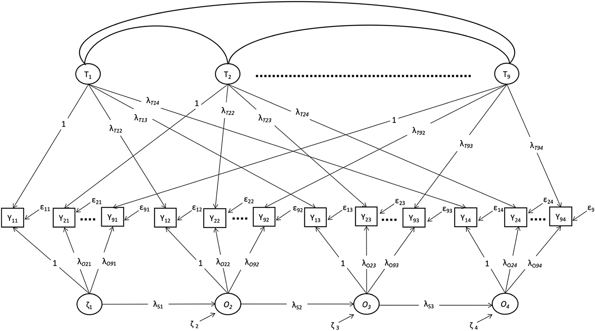
The LST-AR specification is depicted in Fig. 1, which is an adaptation of Fig. 3B of Eid et al. (Reference Eid, Holtmann, Santangelo and Ebner-Priemer2017) for our context where there are nine different observed dichotomous indicators across four occasions. Due to our interest regarding sex differences, a multigroup analysis in males and females was estimated. All analyses were done with Mplus version 8.2 (Muthén & Muthén, Reference Muthén and Muthén2017). The original publication of Eid et al. (Reference Eid, Holtmann, Santangelo and Ebner-Priemer2017) provided details of the specification of LST-AR for continuous indicators; here we gave more details on how to specify the model under dichotomous indicators, where the items' parameters to be estimated are (a) one threshold and (b) one factor loading per item per time. The Mplus syntax for the five models are available in online Supplementary file S1, and the unstandardized estimates for the five models are described in online Supplementary file S2 as a reference for future studies in their model specifications.
LST-AR model with indicator-specific trait variables and congeneric measurement structure for the latent occasion specific residual variables. εit = Measurement error variable of indicator i at time t; λ Tit = regression coefficients of the trait variables of indicator i at time t; λSt = regression coefficients of the common state residual variables at time t; Ot = new residual variables composed of ζt and ζt − 1; Ti = trait variable of indicator i; Yit = observed variable of indicator i at time t; ζ = state residual; λit = loading parameter of the congeneric measurement structure for the latent state variables; λOit = loading parameter of the congeneric measurement structure for the latent occasion residual variables.

Because the observed variables are dichotomous items, we used the weighted least square mean and variance adjusted WLSMV estimator. To scale the latent response factors, we constrained the residual variance of all observed variables to be 1 using Mplus theta parameterization, which gave us equivalent estimates to the traditional graded response model of item response theory (Eid, Reference Eid1996). To obtain an equivalent model, the conditional variances of all latent response have to be fixed (Kamata & Bauer, Reference Kamata and Bauer2008). Takane and de Leeuw (Reference Takane and de Leeuw1987) derived the relation between parameters from standardized confirmatory factor analysis with dichotomous indicators, and used item response theory to show their equivalence. In analyzing dichotomous data with confirmatory factor analysis, the variance of the latent response variables are fixed to 1, and the error variances are freely estimated. In our case, we fixed the error variances to 1, but the variances of the underlying response variables were freely estimated. These are two alternative ways. We chose fixing the error variances because this model is in line with traditional models of item response theory.
The correlations between the indicator-specific trait variables (T i) and the residuals variables (O it and ζ it) were fixed to 0, where i represents the indicator (i.e. item) and t the occasion of measurement (i.e. each wave). It is important to note that according to the LST-AR the trait variables T i represent the trait variables (time-specific dispositions) on the first occasion of measurement. The occasion-specific latent variable Ot is composed of ζ it (the occasion-specific influences on occasion t) and λ S(t−1) ⋅ ζ i(t−1) (indicating carry-over effects). On the first occasion of measurement, the common residual variable is the state residual on the occasion of measurement (ζ i1), whereas subsequently the Ot variables, the composed-occasion residual, are the state residuals plus a linear combination of the previous state residual. Finally, the correlation between the indicator-specific trait variables were freely estimated (i.e. double-headed arrows among all the T latent variables).
For identification purposes the loading of the first indicator on each latent variable was fixed to 1. To test measurement invariance across the four assessments within each cohort and groups, different restrictions were additionally imposed on the parameters of the model. This was conducted to evaluate how both cohorts behave in terms of longitudinal and group invariance concomitantly. As any longitudinal invariance testing (see Millsap, Reference Millsap2010) there are hierarchical steps to follow where restrictions are imposed on the model parameters (i.e. factor loadings, thresholds, factors' variance) progressively. Details about the invariance testing are described in full in online Supplementary Material file S3 to guide the reader about how to proceed with such testing in different situations under LST-AR. Here we will describe exclusively the starting model (called model 0), where no further restrictions were put on the parameters, which, therefore, were freely estimated for both groups and model 1, where the autoregressive from occasion 2 to 3 and 3 to 4, in NCDS, and all the three autoregressive lags in BCS were fixed to be equal within groups (because of similar time lags) but freely estimated between groups.
Evaluation of model fit
We used the following model fit indices to evaluate our model based on the recommendations of Schermelleh-Engel, Kerwer, and Klein (Reference Schermelleh-Engel, Kerwer and Klein2014): χ2-test, comparative fit index (CFI), root mean square error of approximation (RMSEA), and standardized root mean square residual (SRMR). The CFI should be greater than or equal to 0.97. An RMSEA value equal to or smaller than 0.05 indicate a good approximate model fit. The p value of the corresponding test of approximate fit should be equal to or smaller than 0.05. Also, an SRMR smaller than 0.08 would indicate a good fit model. The χ2-difference test using the Mplus DIFFTEST option for WLSMV estimators was applied to test specific restrictions by comparing models being nested within each other, that means that the fit of model 1 against model 0, model 2 against model 1, model 3 against model 2 and so on. If the p value of the χ2-difference test was equal to or smaller than 0.05 the more restricted model was rejected.
Derived indices from LST-AR
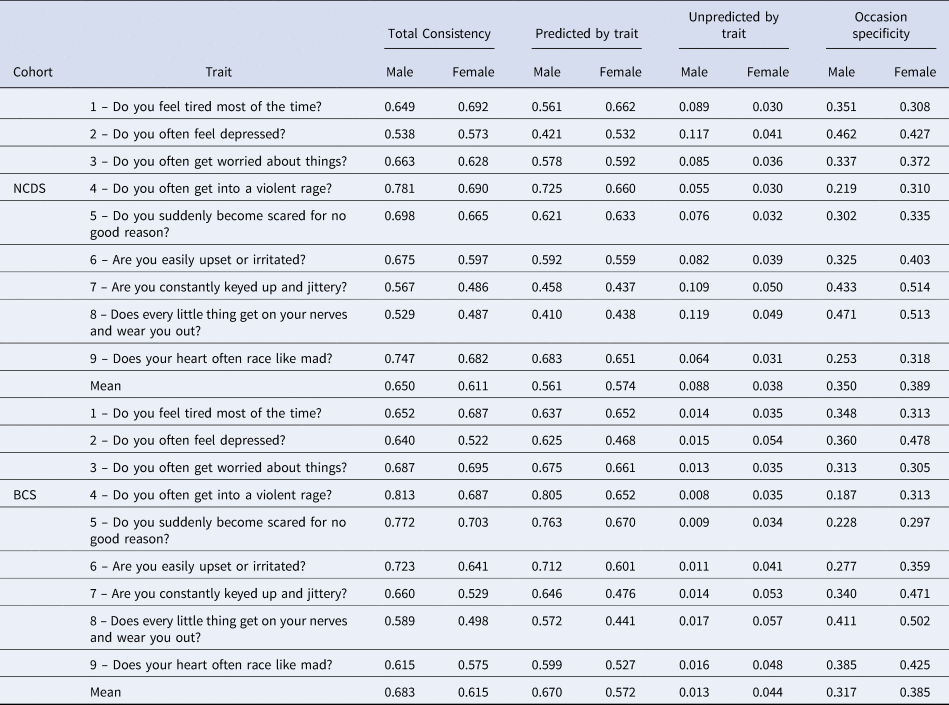
Based on Eid et al. (Reference Eid, Holtmann, Santangelo and Ebner-Priemer2017) four indices were computed: consistency indicating the amount of stability, and occasion specificity representing the amount of variability (instability). The consistency coefficient was additionally decomposed into a coefficient indicating the predictability by the trait (on the first occasion of measurement) and the unpredictability by the trait (on the first occasion of measurement). The latter is a proportion of variation coming from the autoregressive effect, which indicates a carry-over effect or more precisely an accumulated situational influence.
Missing data
Assuming multivariate normally distributed latent variables, the WLSMV estimator, which is a limited information estimator, uses only the univariate and bivariate information during the parameter estimation process (i.e. the observed univariate marginal frequencies and observed bivariate frequencies of the categorical indicators) (see Forero & Maydeu-Olivares (Reference Forero and Maydeu-Olivares2009). Under WLSMV, the missing data might be dealt under pairwise deletion (the default function in Mplus) or listwise deletion. Here we opted for pairwise deletion, preserving a greater number of subjects in the analysis and consequently and avoiding selection bias related to listwise deletion (Little, Reference Little1992; Peugh & Enders, Reference Peugh and Enders2004).
Results
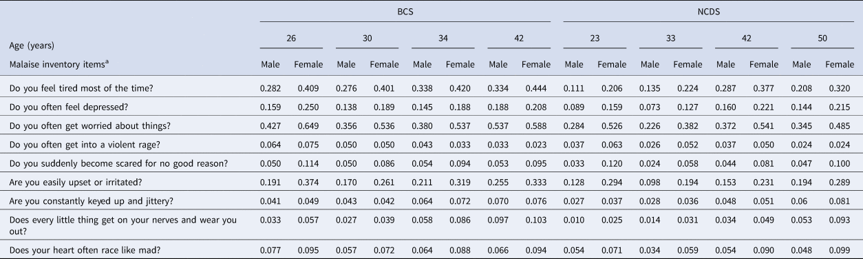
For these analyses, the sample comprised a total of 11 174 (54% female and 46% male) adults followed from 23 to 50 years of age. Descriptive statistics for the prevalence of psychological distress symptoms, indicated by positive responses to the nine items of the Malaise Inventory, are depicted by age and sex across the four waves in Table 1. The most prevalent symptoms of psychological distress across both cohorts and sexes were getting worried about things and feeling tired most of the time.
Prevalence of symptoms of psychological distress across the time by sex in both cohorts

BCS, British cohort study; NCDS, National Child Development Study.
a Prevalence from the longitudinal sample of answer ‘Yes’ to item.
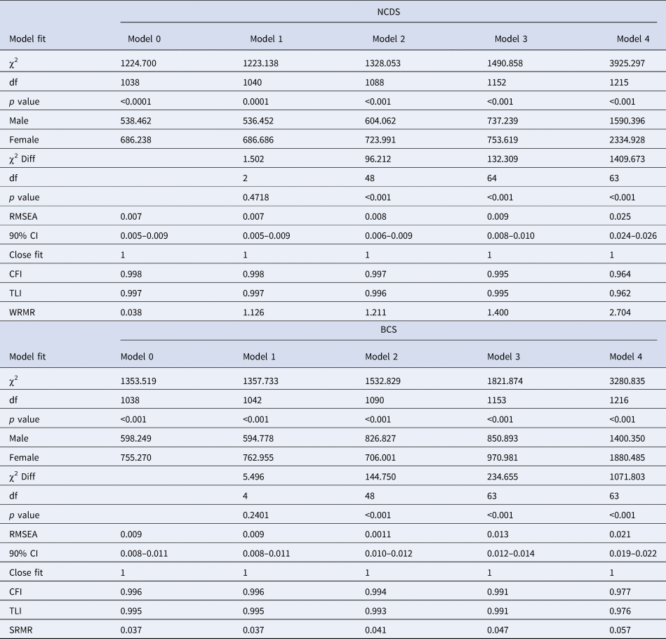
Table 2 shows the model fit indices across the five specified models. In both cohorts model 1 did not fit worse than model 0, but all other more restricted models fit significantly worse; therefore, we chose model 1 as the best fitting model. Although the other more constrained models showed very good approximate fits per se in both cohorts, indicating that the measurement invariance assumptions were violated only slightly, we based all further analyses on the parameters of model 1 to avoid any parameter bias.
Model fit indices for the LST-AR models

BCS, British cohort study; CI, confidence interval; CFI, confirmatory factor index; df, degrees of freedom; Diff, difference; LST-AR, latent-state-trait model with autoregressive effect; NCDS, National Child Development Study; RMSEA, root mean square error of approximation; TLI, Tucker–Lewis index.
Model 0 no constrains across the groups; Model 1 constrains in autoregressive effects; Model 2 measurement invariance across the time; Model 3 measurement across time and group; Model 4 thresholds held equal across time and across the groups.
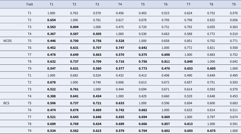
Table 3 shows the correlations between indicator-specific trait variables for males and females. In bold, below the diagonal, the trait correlations for males are presented whereas the non-bold results refer to the traits correlations for females. The large range of correlations indicates that the items were not unidimensional and item-specific effects have to be considered. The highest correlation was between T7 (Are you constantly keyed up and jittery) and T8 (Does every little thing get on your nerves and wear you out?) for NCDS58 and T6 (Are you easily upset or irritated?) and T8 (Does every little thing get on your nerves and wear you out?) for BCS70. The lowest correlation was between T1 (Do you feel tired most of time?) and T4 (Do you often get into a violent rage?) for both cohorts.
Trait correlations in both cohorts (in bold correlation among male group)

BCS, British cohort study; NCDS, National Child Development Study; T1, Do you feel tired most of the time?; T2, Do you often feel depressed?; T3, Do you often get worried about things?; T4, Do you often get into a violent rage?; T5, Do you suddenly become scared for no good reason?; T6, Are you easily upset or irritated?; T7, Are you constantly keyed up and jittery?; T8, Does every little thing get on your nerves and wear you out?; T9, Does your heart often race like mad?
In bold, below the diagonal, there is the indicator-specific trait correlation matrix for male and in non-bold for female.
Table 4 presents the four components derived from the LST-AR model calculated on the basis of the estimated model parameters of the last wave in order to estimate the influence of accumulated situational influences over the whole period (variance components for the other waves can be obtained from the corresponding author on request). In both cohorts, comparing consistency and occasion specificity coefficients (which summed up to 1) showed that among males and females the amount of consistency (stability) was larger than the amount of variability across the nine traits (i.e. after the modeling, each item is representing a trait) across both cohorts with the exception of item 8 in the NCDS and BCS female group and item 7 in the NCDS female group. This means that there is in general a higher degree of stability than of variability. Comparing males and females in terms of consistency, the degree of stability across all the nine traits, on average and in terms of point estimate, for both cohorts, was larger among males when compared to females (on average NCDSmale = 0.650 v. NCDSfemale = 0.611; BCSmale = 0.683 v. BCSfemale = 0.615). Occasion specificity in both cohorts was larger among females (on average for both cohorts of 0.387) when compared to males (on average 0.333).
Consistency and occasion-specific residual at the fourth wave of assessment for both cohorts

BCS, British cohort study; NCDS, National Child Development Study.
Disentangling the consistency coefficients, the accumulated situational effects (i.e. evaluated by the unpredictability by the trait) were systematically larger for males in the older cohort (NCDS58). This effect changed in BCS70, where the accumulated situational effect was stronger for females than males across all the psychological distress traits. However, in both sexes individual differences on an occasion of measurement were generally much more strongly determined by trait differences (on the first occasion of measurement) than by accumulated situational effects, showing that there is strong trait stability over time. Lastly, online Supplementary Material 4 reports the reliabilities (i.e. R 2) for the nine items, across the four times, per sex and cohort.
Discussion
Applying revised LST theory, we decomposed nine psychological distress indicators into consistency, which is a proportion of variance due to trait difference, and occasion specificity (instability). The former indicated that the largest amount of variance on an occasion of measurement in both sexes is due to individual trait differences and not to occasion-specific influences. This result was found in both cohorts showing high replicability, and indicating that the reported between-cohort differences are not due to period effects (Ploubidis et al., Reference Ploubidis, Sullivan, Brown and Goodman2017). When decomposing the consistency coefficient into two parts, the proportion of variance explained by the trait (on the first occasion of measurement) was much larger than the variance due to accumulated situational effects; an individual predisposed to distress remained more likely to be distressed.
In terms of decomposing psychological distress into state and trait variances, one pioneer work was conducted in a sample of Dutch adults aged 22–65, using a stability and change model (Ormel & Schaufeli, Reference Ormel and Schaufeli1991). The authors examined 226 subjects across three timepoints over a 7-year period. That model presumes that each person has a ‘stable and characteristic symptom level’ that interacts with the environment in a dynamic and synergistic mechanism that tries to compensate for perturbations created by change agents, which include personality traits. The authors applied this model to investigate two personality trait-like characteristics, self-esteem and locus of control, and their contamination by the psychological distress level, including parameters for symptom stability, an (autoregressive) change component of symptoms, representing effects of transitory components, and measurement error. The study found correlations between the measures of distress and personality, explained by effects of symptom change on self-esteem and the correlation between trait self-esteem and stable symptom levels.
The consistency of psychological distress symptoms tended to rise between subjects born in 1958 (NCDS58) and those born in 1970 (BCS70) due to trait differences throughout adult life. Previously, an increase in psychological distress in midlife between these two cohorts was observed, which was more pronounced in men (Ploubidis et al., Reference Ploubidis, Sullivan, Brown and Goodman2017) and could not be explained by early-life influences. Here we add that the nature of these symptoms was also changing, indicating an increase in trait/consistent variance which can be attributed to cohort effects between these generations.
In psychiatry, trait and state aspects of symptoms are commonly discussed, but rarely evaluated in statistical models (Conway, Hipwell, & Stepp, Reference Conway, Hipwell and Stepp2017; Steyer et al., Reference Steyer, Ferring and Schmitt1992). Mood disorders tend to be episodic, in other words, occasion specific, involving some level of symptomatology that changes dynamically from episode to remission, although there might also be a much stronger component that remains constant despite periods of remission and a component that depends on the severity of previous mood episodes over time (Kovacs, Obrosky, & George, Reference Kovacs, Obrosky and George2016). In major depression, for instance, serotonin dysregulation that is found in acute patients (Sargent et al., Reference Sargent, Kjaer, Bench, Rabine, Messa, Meyer and Cowen2000) persists until recovery from depression (Bhagwagar & Cowen, Reference Bhagwagar and Cowen2008). Gamma-aminobutyric acid (GABA) availability, secretion of cortisol, and monoamine oxidase levels have also been suggested as trait markers of vulnerability to depression based on abnormalities found even in recovered depressed patients (Bhagwagar & Cowen, Reference Bhagwagar and Cowen2008; Meyer et al., Reference Meyer, Wilson, Sagrati, Miler, Rusjan, Bloomfield and Houle2009). Although these mood-related biological mechanisms have been extensively discussed (Wang et al., Reference Wang, Zhou, Zhu, Wang, Fang, Zhong and Xie2016), trait and state aspects have not been evaluated formally in longitudinal structural equation models.
Some studies have used LST-theory to disentangle state and trait components using biological data, such as cortisol based on multi-state single-trait models from two parallel measures (Hellhammer et al., Reference Hellhammer, Fries, Schweisthal, Schlotz, Stone and Hagemann2007) and electroencephalogram data (Hagemann, Hewig, Seifert, Naumann, & Bartussek, Reference Hagemann, Hewig, Seifert, Naumann and Bartussek2005) applying a true (error-free) intraindividual change model that considers latent state changes between occasions. LST modeling was also applied to investigate trait specificity and network connectivity reliability on resting state functional magnetic resonance imaging condition, for different task conditions (Li et al., Reference Li, Vidorreta, Katchmar, Alsop, Wolf and Detre2018). These previous studies showed innovative ways of dealing with repeated (discrete) measures across time, but the LST approach remains uncommon.
The course and outcome of mental disorders play important roles in validating psychiatric taxonomy. Onset, duration, and recurrence of episodes and long-term outcome make up the scenarios that guide studies in the elaboration of an etiological model of disease (Kendall et al., Reference Kendall, Zinbarg, Mineka, Bobova, Prenoveau, Revelle and Craske2015). Clinically, symptoms are not equally stable across time; there can be differences in the frequency, duration, and intensity of individual symptoms over the course of the disease. Sub-clinical mood symptoms, alone or in constellations, may also contribute to inter-individual differences in malaise, and to the relative consistency of psychological symptoms over time. Although the current study adopted non-specific psychological symptoms, the LST model has been applied to investigate the impact of trait-like personality characteristics and cognitive bias as predictors of depression outcomes, finding that depressive symptoms predicted cognitive bias (LaGrange et al., Reference LaGrange, Cole, Jacquez, Ciesla, Dallaire, Pineda and Felton2011). These and other factors influence the amount and trajectory of mood symptoms in the general population, quantified here in terms of their trait, autoregressive (accumulative effects), and occasion-specific features. Further studies might compare the relative consistency of psychological traits between people with and without mood disorders and determine to what extent the presence of a mood disorder contributes to the consistency of these symptoms at the population level.
Fundamental concepts, such as ‘chronicity,’ are widely applied without a model that isolates the signal of enduring phenomena amid bias caused by transitory events. Conway, Rutter, and Brown (Reference Conway, Rutter and Brown2016) fit a latent TSO model to map the trajectory of depression as a function of chronic (time-invariant) stressors, finding stress chronicity was associated with a more refractory course of depression. Theoretical models of the consequences of childhood adversity on depressive disorders have also been investigated after disentangling state and trait effects, to examine the impact of stable stress processes on external stress-dependent constructs (Cole, Nolen-Hoeksema, Girgus, & Paul, Reference Cole, Nolen-Hoeksema, Girgus and Paul2006; Cole et al., Reference Cole, Martin, Jacquez, Tram, Zelkowitz, Nick and Rights2017; Conway et al., Reference Conway, Hipwell and Stepp2017; Donnellan, Kenny, Trzesniewski, Lucas, & Conger, Reference Donnellan, Kenny, Trzesniewski, Lucas and Conger2012).
Generally, our data showed that psychological symptoms exhibited greater stability among men than women, with the exception of tiredness (higher consistency among women in both cohorts) and possibly depression (higher among women in NCDS but not in BCS). Differences in the prevalence of major depression and other psychiatric disorders between men and women are well documented. Depression is more prevalent in females, and frequently accompanied by anxiety (Fried, Epskamp, Nesse, Tuerlinckx, & Borsboom, Reference Fried, Epskamp, Nesse, Tuerlinckx and Borsboom2016; Kessler, Zhao, Blazer, & Swartz, Reference Kessler, Zhao, Blazer and Swartz1997; Labaka, Goñi-Balentziaga, Lebeña, & Pérez-Tejada, Reference Labaka, Goñi-Balentziaga, Lebeña and Pérez-Tejada2018; Salk et al., Reference Salk, Hyde and Abramson2017) with increased vulnerability emerging by age 13–15 (de Kruif et al., Reference de Kruif, Spijker and Molendijk2016; Salk et al., Reference Salk, Hyde and Abramson2017). Longitudinal studies have noted higher frequencies of malaise in woman than men, with a stable trend suggesting trait-like phenomenology (Furnham & Cheng, Reference Furnham and Cheng2015), however no study examined differences in trait and occasion specific sources of variance between the sexes at the population level.
Contrary to the present findings in adulthood, both negative and positive cognitions were more consistent among girls than boys, and boys had more occasion specific variance for negative cognitions (Cole et al., Reference Cole, Jacquez, Truss, Pineda, Weitlauf, Tilghman-Osborne and Maxwell2009) among a school-based sample. That study applied the TSO proposed by Cole et al. (Reference Cole, Martin and Steiger2005) model to items of self-reported competence, which includes self-esteem. Therefore, it is possible that sex differences are conditional upon age or developmental stage, which might be investigated further.
In one study, developmental relationships between depressive symptoms and stressful events from adolescence through age 30 was tested using an autoregressive latent trajectory (Pettit, Lewinsohn, Seeley, Roberts, & Yaroslavsky, Reference Pettit, Lewinsohn, Seeley, Roberts and Yaroslavsky2010), a combination of autoregressive (simplex) model and the latent trajectory (curve) model, based on the model specification of Bollen and Curran (Reference Bollen and Curran2004). They found that the latent trajectory of depressive symptoms was nonlinear, decreasing through adolescence to adulthood, and that higher trait levels of hassles in woman were associated with slower rates of decrease in depressive symptoms (Pettit et al., Reference Pettit, Lewinsohn, Seeley, Roberts and Yaroslavsky2010).
As a possible limitations, the nine questions to investigate five clusters of symptoms were addressed by the Malaise Inventory, of these, three symptoms are DSM criteria (i.e. energy loss, sadness, and agitation) and two are not, comprising irritability and pessimism clusters, therefore, the results to not map onto DSM diagnostic criteria for a psychiatric disorder; however, the validity of the Malaise Inventory to assess the construct of psychological distress has been well-validated (Grant et al., Reference Grant, Nolan and Ellis1990; Hirst & Bradshaw, Reference Hirst and Bradshaw1983; McGee et al., Reference McGee, Williams and Silva1986; Ploubidis, McElroy, & Moreira, Reference Ploubidis, McElroy and Moreira2019; Rodgers et al., Reference Rodgers, Pickles, Power, Collishaw and Maughan1999) and predictive of health outcomes (Furnham & Cheng, Reference Furnham and Cheng2015; Ploubidis et al., Reference Ploubidis, Sullivan, Brown and Goodman2017). Direct comparisons between the various indices in the two cohorts (consistency and occasion specificity) should be interpreted with caution because NCDS and BCS were run separately, so invariance testing and constraints between the cohorts were not added in the modeling. Lastly, in terms of missing data at the item level, the WLSMV estimator operates via pairwise deletion (i.e. computing each covariance on the basis of all cases with non-missing values for that particular pair of variables, see Marsh, Reference Marsh1998), thus, preserving more subjects being analyzed when compared with listwise deletion; however, WLSMV assumes a missing-completely-at-random mechanism, which might be considered as a mechanism with stronger assumptions (Marsh, Reference Marsh1998).
Conclusions
In two birth cohorts, each with almost 50 years of follow-up data, approximately two-thirds of the information in nine indicators of psychological distress was trait-like, being present already at the first occasion of measurement in early adulthood. Approximately one-third of the variance was occasion-specific, while ~5% of the variability was due to accumulated situational effects. An enduring predisposition to psychological distress plays a fundamental role in its manifestations across adult life.
Supplementary material
The supplementary material for this article can be found at https://doi.org/10.1017/S0033291719003805.
Acknowledgements
We are grateful to all participants of the NCDS and BCS study.
Financial support
The research producing the results reported in this paper was sponsored by the Coordenação de Aperfeiçoamento de Pessoal de Nível Superior (CAPES) scholarship program (Finance Code 001), and a partnership between the Center for Longitudinal Studies/SPRINT and Fundação de Amparo à Pesquisa do Estado de São Paulo (FAPESP) (2016/50195-0). H.C-M. is thankful to CAPES Thesis Award (No. 0374/2016, Process No. 23038.009191/2013-76) and to the senior researcher CAPES-Alexander von Humboldt Foundation Post-Doc Fellowship (Process number 88881.145593/2017-01). G.B.P. was supported by the Economic and Social Research Council (ES/M008584/1). Dr Swardfager acknowledges support from the Canadian Institutes of Health Research, and the National Sciences and Engineering Research Council of Canada, and support from the Department of Psychiatry, Sunnybrook Health Sciences Centre. The NCDS and BCS study was supported by Centre for Longitudinal Studies and University College of London (UCL). This manuscript reflects the views of the authors and may not reflect the opinions or views of the National Child Development Study or 1970 British Cohort Study investigators or the Centre for Longitudinal Studies.
Conflict of interest
None.
Ethical standards
The authors assert that all procedures contributing to this work comply with the ethical standards of the relevant national and institutional committees on human experimentation and with the Helsinki Declaration of 1975, as revised in 2008.