



1. Introduction
The stability of oscillating liquid films, a key branch of flow stability, possesses significant industrial relevance. Applications include coating processes (Weinstein & Ruschak Reference Weinstein and Ruschak2004), heat and mass transfer enhancement in heat exchangers (Yoshimura, Nosoko & Nagata Reference Yoshimura, Nosoko and Nagata1996; Bender, Stephan & Gambaryan-Roisman Reference Bender, Stephan and Gambaryan-Roisman2017) and fuel atomisation in aerospace engines (Woods & Lin Reference Woods and Lin1995). For instance, maintaining liquid film stability is critical for ensuring coating quality in processes like dip coating and microfluidic chip etching. However, mechanical vibrations in coating equipment and low-frequency resonance in etching tools, which are often unavoidable, severely compromise film formation quality (Skardak Reference Skardak2001; Gao & Lu Reference Gao and Lu2008). Conversely, actively applying controlled oscillatory fields allows manipulation of instability patterns, enabling targeted promotion or suppression. The foundational theoretical work of Yih (Reference Yih1963) established the inherent instability of liquid films. To effectively control stability in such intrinsically unstable systems, the introduction of external forces, such as periodic oscillations in the direction parallel to the flow, becomes essential (Lin, Chen & Woods Reference Lin, Chen and Woods1996).
Research on the stability of vertically oscillated liquid films has advanced significantly since Faraday’s seminal experiments (Faraday Reference Faraday1831). This study, however, primarily focuses on the impact of streamwise oscillations on the stability of horizontal liquid films. Seminal work by Yih (Reference Yih1968) applied a streamwise-periodic oscillation to the bottom wall, generating a time-dependent basic flow. Employing long-wave asymptotic analysis, Yih (Reference Yih1968) solved the Orr–Sommerfeld eigenvalue problem with periodic coefficients, uncovering an instability mode linked to surface deformation, termed the Yih mode. The analysis demonstrated that, in the absence of gravity, long-wave instability depends solely on oscillation frequency. Inclusion of gravity introduces a critical amplitude for instability, which increases with oscillation frequency. Or (Reference Or1997) extended Yih’s analysis to perturbations of arbitrary wavenumber. By numerically solving the Orr–Sommerfeld equations, they mapped out the critical instability amplitude (measured by the Reynolds number) as a function of frequency, revealing neutral curves across the entire parameter plane. Their results showed a branching point near the rapidly growing long-wave neutral curve where finite-wavelength instability dominates, and at certain frequencies, finite-wavelength instability is favoured over long-wave modes. Motivated by these findings, researchers have explored diverse control strategies, such as surfactants (Gao & Lu Reference Gao and Lu2006, Reference Gao and Lu2008), viscoelasticity (Dandapat & Gupta Reference Dandapat and Gupta1975; Samanta Reference Samanta2017; Wang et al. Reference Wang, Du, Xiao and Zhao2023) and external electric fields (Samanta Reference Samanta2009, Reference Samanta2019). Recently, Jaouahiry & Aniss (Reference Jaouahiry and Aniss2025) systematically investigated dual-frequency wall oscillations, modelling coating process oscillations more realistically. Combining long-wave expansion and Chebyshev spectral methods, they analysed the interlink between long-wave and finite-wavelength instabilities and determined critical amplitudes and wavenumbers across various amplitude ratios.
Beyond the above approaches, alternative modulation strategies for oscillating liquid film instabilities have attracted increasing interest. Modifying the geometric confinement of vibrating plates presents one such avenue. Experimental and numerical studies have shown that sidewalls significantly suppress falling liquid film instabilities (Kögel & Aksel Reference Kögel and Aksel2020; Mohamed, Sesterhenn & Biancofiore Reference Mohamed, Sesterhenn and Biancofiore2023). This finding strongly suggests a potentially critical influence of sidewalls on the stability of oscillating liquid films under analogous confinement. It is worth noting that the stability of oscillatory flows in multi-layer systems has also been investigated. Khenner et al. (Reference Khenner, Lyubimov, Belozerova and Roux1999) examined the stability of plane-parallel vibrational flow in a two-layer system, considering the interface between two immiscible fluids in a horizontally oscillating cavity. Their analysis revealed parametric resonant instabilities associated with capillary-gravity waves at the interface, with the inviscid case reducible to the Mathieu equation. Lyubimov et al. (Reference Lyubimov, Ivantsov, Lyubimova and Khilko2016) performed direct numerical simulations of frozen wave formation at the interface of fluids with high viscosity contrast under horizontal vibrations, analysing both the critical conditions for wave formation and the structure of average flows. These studies provide valuable insights into oscillatory interfacial instabilities in confined geometries. Furthermore, vibration-induced effects on thin film stability extend beyond simple horizontal oscillations. Shklyaev, Alabuzhev & Khenner (Reference Shklyaev, Alabuzhev and Khenner2009) investigated the influence of longitudinal and tilted vibrations on film stability and dewetting, demonstrating that, while longitudinal vibrations destabilise planar films, tilted vibrations can either stabilise or destabilise depending on the configuration, with potential applications in micro-particle transport.
For confined films, the basic flow deviates from Nusselt’s parallel flow approximation (Nusselt Reference Nusselt1916), featuring a two-dimensional spatial distribution dependent on both the wall-normal and spanwise coordinates. Accurately determining this flow and specifying the contact angle boundary condition at the sidewall three-phase contact line pose significant challenges. Fulford (Reference Fulford1962, Reference Fulford1964) conducted early comprehensive reviews of theoretical and experimental work on thin films in rectangular channels, discussing sidewall contact angle effects on the velocity profile. Scholle & Aksel (Reference Scholle and Aksel2001) incorporated capillarity, detailing exact solution procedures for the basic flow and emphasising sidewall effects on velocity structure and capillary rise. Later, Haas, Pollak & Aksel (Reference Haas, Pollak and Aksel2011) employed combined theory and experiment to study gravity-driven films, highlighting the dual role of sidewall no-slip conditions (reducing velocity) and capillarity (increasing velocity near the wall).
Regarding stability analysis of sidewall-confined falling films, Vlachogiannis et al. (Reference Vlachogiannis, Samandas, Leontidis and Bontozoglou2010) experimentally observed that the critical Reynolds number of long-wave instability decreases with increasing channel width, approaching two-dimensional theory predictions as sidewall influence diminishes. Georgantaki et al. (Reference Georgantaki, Vatteville, Vlachogiannis and Bontozoglou2011) experimentally demonstrated that the significance of sidewalls depends on fluid properties: higher Kapitza numbers correlate with significant film height bending near walls, while lower Kapitza numbers result in less curvature, approaching a two-dimensional instability mode. Pollak, Haas & Aksel (Reference Pollak, Haas and Aksel2011) investigated sidewall contact angle effects, finding that surface instabilities consistently transition from long-wave to short-wave modes regardless of contact angle when the sidewall distance is reduced. More recently, Kögel & Aksel (Reference Kögel and Aksel2020) experimentally detected neutral curve fragmentation at intermediate disturbance frequencies, tentatively attributing it to selective sidewall damping. Mohamed et al. (Reference Mohamed, Sesterhenn and Biancofiore2023) subsequently provided a detailed explanation through experiment and simulation, identifying two distinct modes in open channel stability: traditional hydrodynamic modes and wall modes induced by sidewalls. Narrowing the channel suppresses the hydrodynamic mode, leaving the less sensitive wall mode dominant, thereby fragmenting the neutral curve.
In summary, compelling evidence confirms that sidewalls exert a pronounced suppressive effect on surface wave instability modes in falling liquid films. This well-established finding in one class of film flows naturally prompts a fundamental question: Are the classical instabilities inherent to horizontally oscillating liquid films similarly susceptible to suppression by sidewalls? Despite the extensive literature on both confined falling films and unconfined oscillating films, this question remains unexplored. In the present study, we extend the foundational two-dimensional model of horizontally oscillating liquid films pioneered by Yih (Reference Yih1968) into a three-dimensional framework specifically designed to probe the influence of sidewall spacing. The introduction of oscillating sidewalls significantly increases the complexity of the stability problem. Specifically, owing to lateral confinement by the sidewalls and their associated boundary conditions, disturbances can no longer be assumed to be strictly spanwise periodic. The fundamental time dependence of the base flow does not invalidate the assumption of exponentially growing or decaying perturbations; this behaviour remains valid with time-periodic flows, as captured by the modes specified in Floquet theory. Consequently, a sophisticated bi-global instability analysis (Theofilis Reference Theofilis2011) becomes necessary to capture the complete coupling between the evolving base flow and infinitesimal disturbances. This study goes beyond establishing a qualitative stabilisation trend. By leveraging this bi-global Floquet framework, we specifically investigate: (i) the emergence of distinct three-dimensional instability modes induced by lateral confinement; (ii) the symmetry properties and competition between these modes as the primary mechanism for stabilisation; and (iii) the quantitative energy transfer pathways that sustain each mode. This computational task is considerably more demanding than typical bi-global stability studies due to the combined challenge of spatial non-uniformity and temporal periodicity. The novel computational challenge lies in solving the resulting high-dimensional eigenvalue problem derived from the bi-global analysis. This complexity ultimately manifests as the need to solve a very large, complex coefficient matrix eigenvalue problem. Extending an efficient and robust methodology to tackle this large-scale eigenvalue problem is a key aspect of this work.
The outline of the remainder of this investigation is presented as follows. Section 2 presents the mathematical formulation for confined oscillating films. The linear stability problem is addressed in § 3, where Floquet-based perturbation equations are derived using bi-global analysis. The resolution of long-wave instabilities in § 4 is achieved using a semi-analytical asymptotic approach through perturbation expansions. In § 5, the eigenvalue problem for arbitrary wavenumbers is solved through a numerical procedure employing Chebyshev spectral collocation methods. Parametric studies are conducted in § 6 to quantify sidewall effects on neutral curves and to elucidate different modes. Finally, distinct instability mechanisms are revealed in § 7 using energy budget analysis.
2. Mathematical formulation
2.1. Flow configuration
Consider a three-dimensional incompressible Newtonian liquid film within a horizontally oscillating channel of width
 $W^*$
, as illustrated in figure 1. A Cartesian coordinate system
 $(x^*, y^*, z^*)$
is adopted, where
 $x^*$
denotes the streamwise direction along the flow,
 $y^*$
is perpendicular to the bottom wall and
 $z^*$
represents the spanwise direction. The superscript ‘
 $*$
’ designates dimensional variables. The sidewalls are located at
 $z^* = 0$
and
 $z^* = W^*$
, respectively. The film thickness, denoted
 $h^*(x^*, z^*, t^*)$
, varies with position and time. The equilibrium film thickness at rest is
 $d$
, indicated by the dashed line in figure 1. The density
 $\rho$
and kinematic viscosity
 $\nu$
of the incompressible Newtonian fluid are assumed constant. A streamwise-periodic oscillation
 $U^*_0\cos (\omega ^* t^*)$
, characterised by amplitude
 $U^*_0$
and angular frequency
 $\omega ^*$
, is imposed on both the bottom wall and the sidewalls. The motion of the three-dimensional incompressible Newtonian fluid is governed by the following equations in the Cartesian coordinate system:
 \begin{align} \boldsymbol{\nabla } \boldsymbol{\cdot } \boldsymbol{u}^* &=0, \end{align}
 \begin{align} \partial _{t^*}u^*+\boldsymbol{u}^*\boldsymbol{\cdot }\boldsymbol{\nabla } u^* &=-\rho ^{-1}\partial _{x^*}p^*+\nu {\nabla} ^{2}u^*, \end{align}
 \begin{align} \partial _{t^*}v^*+\boldsymbol{u}^*\boldsymbol{\cdot }\boldsymbol{\nabla } v^* &=-\rho ^{-1}\partial _{y^*}p^*+\nu{\nabla} ^{2}v^*-g, \end{align}
 \begin{align} \partial _{t^*}w^*+\boldsymbol{u}^*\boldsymbol{\cdot }\boldsymbol{\nabla } w^* &=-\rho ^{-1}\partial _{z^*}p^*+\nu {\nabla} ^{2}w^*, \end{align}
where
 $\boldsymbol{u}^* = (u^*, v^*, w^*)$
represents the velocity vector, with components
 $u^*$
,
 $v^*$
and
 $w^*$
corresponding to the
 $x^*$
,
 $y^*$
and
 $z^*$
directions,
 $g$
is the acceleration of gravity, respectively.
Schematic diagram of liquid film flow in a streamwise oscillating channel.

The corresponding boundary conditions are formulated as follows:
-
(i) At the sidewalls
 $z^* = 0$
and
$z^* = W^*$
, and the bottom wall
$y^* = 0$
, the no-slip and no-penetration conditions are prescribed(2.2)
\begin{equation} u^* = U_0^* \cos (\omega ^* t^*), \quad v^* = 0, \quad w^* = 0. \end{equation}
-
(ii) The kinematic condition at the free surface
$y^* = h^*(x^*, z^*, t^*)$
is given by(2.3)
\begin{equation} \partial _{t^*} h^* + \boldsymbol{u}^* \boldsymbol{\cdot } \boldsymbol{\nabla } h^* = v^*. \end{equation}
-
(iii) The stress balance at the free surface
$y^* = h^*(x^*, z^*, t^*)$
yields(2.4)
\begin{align} \boldsymbol{n} \boldsymbol{\cdot } \big(\unicode{x1D64F}^{{{\kern1pt}}*} -\unicode{x1D64F}^{{{\kern1pt}}*}_\infty \big) \boldsymbol{\cdot } \boldsymbol{n} &= 2 \sigma ^* K(h^*), \end{align}
(2.5)
\begin{align} \boldsymbol{t}_1 \boldsymbol{\cdot } \big(\unicode{x1D64F}^{{{\kern1pt}}*} -\unicode{x1D64F}^{{{\kern1pt}}*}_\infty \big) \boldsymbol{\cdot } \boldsymbol{n} &= 0, \end{align}
(2.6)
\begin{align} \boldsymbol{t}_2 \boldsymbol{\cdot } \big(\unicode{x1D64F}^{{{\kern1pt}}*} -\unicode{x1D64F}^{{{\kern1pt}}*}_\infty \big) \boldsymbol{\cdot } \boldsymbol{n} &= 0, \end{align}


where
 $\unicode{x1D64F}^{{{\kern1pt}}*} = -p^*\unicode{x1D644} + 2 \mu\unicode{x1D640}^{{{\kern1pt}}*}$
is the fluid stress tensor,
 $\sigma ^*$
is the surface tension coefficient,
 $p^*$
denotes the isotropic pressure,
 $\unicode{x1D644}$
is the identity tensor and
 $\unicode{x1D640}^{{{\kern1pt}}*} = ({1}/{2}) (\boldsymbol{\nabla } \boldsymbol{u}^* + (\boldsymbol{\nabla } \boldsymbol{u}^*)^{\mathrm{T}})$
represents the strain rate tensor. For a gaseous environment, at the free surface we have
 $\boldsymbol{T}^*_\infty = -p_\infty \boldsymbol{I}$
, where
 $p_\infty$
represents atmospheric pressure. The unit normal vector
 $\boldsymbol{n}$
, and the unit tangent vectors
 $\boldsymbol{t}_1$
(streamwise) and
 $\boldsymbol{t}_2$
(spanwise) define the free-surface orientation. The mean curvature
 $K(h^*)$
is defined as
 $K = ({1}/{2})(k_1 + k_2) =({1}/{2})(1/R_1 + 1/R_2)$
. For detailed derivations, refer to Kalliadasis et al. (Reference Kalliadasis, Ruyer-Quil, Scheid and Velarde2011).
The governing equations and boundary conditions are normalised using the following characteristic scales: the equilibrium film thickness
 $d$
for length,
 $\nu /d$
for velocity,
 $1/\omega ^*$
for time and
 $\rho \nu ^2/d^2$
for pressure. This yields the dimensionless parameters
 \begin{equation} \beta =\sqrt {\frac {\omega ^* d^2}{2\nu }}, \quad Re=\frac {U_0^{*}d}{\nu }, \quad \chi =\frac {g d^3}{2\nu ^2}, \quad{\textit{We}}= \frac {\sigma ^* d}{\rho \nu ^2}, \quad W = \frac {W^*}{d}, \end{equation}
where the Womersley number
 $\beta$
characterises the ratio of film thickness to Stokes boundary layer thickness,
 $ Re$
is the Reynolds number representing oscillation amplitude effects, the Galileo number
 $\chi$
quantifies gravitational versus viscous forces,
 $We$
denotes the Weber number for surface tension effects and
 $W$
is the dimensionless channel width.
The dimensionless equations are
 \begin{align} \boldsymbol{\nabla } \boldsymbol{\cdot } \boldsymbol{u} &= 0, \end{align}
 \begin{align} 2\beta ^2\partial _{t}u + \boldsymbol{u} \boldsymbol{\cdot } \boldsymbol{\nabla } u &= -\partial _{x}p + {\nabla} ^{2}u, \end{align}
 \begin{align} 2\beta ^2\partial _{t}v + \boldsymbol{u} \boldsymbol{\cdot } \boldsymbol{\nabla } v &= -\partial _{y}p + {\nabla} ^{2}v - 2\chi , \end{align}
 \begin{align} 2\beta ^2\partial _{t}w + \boldsymbol{u} \boldsymbol{\cdot } \boldsymbol{\nabla } w &= -\partial _{z}p + {\nabla} ^{2}w. \end{align}
The dimensionless boundary conditions at the bottom wall and sidewalls are
 \begin{equation} u ={\textit{Re}}\cos t, \quad v = 0, \quad w = 0. \end{equation}
The kinematic condition at the free surface becomes
 \begin{equation} 2\beta ^2\partial _{t} h + \boldsymbol{u} \boldsymbol{\cdot } \boldsymbol{\nabla } h = v. \end{equation}
The normal and tangential stress balances at the free surface are
 \begin{align} p &= \frac {2}{n^{2}} \Big [ (\partial _{x}h)^2 \partial _{x}u + (\partial _{z}h)^2 \partial _{z}w + \partial _{x}h \partial _{z}h (\partial _{z}u + \partial _{x}w) \notag \\ &\quad - \partial _{x}h (\partial _{y}u + \partial _{x}v) - \partial _{z}h (\partial _{z}v + \partial _{y}w) + \partial _{y}v \Big ] \notag \\ &\quad - \frac {\textit{We}}{n^{3}} \Big [ \partial _{\textit{xx}}h \big(1 + (\partial _{z}h)^2\big) + \partial _{\textit{zz}}h \big(1 + (\partial _{x}h)^2\big) - 2 \partial _{x}h \partial _{z}h \partial _{xz}h \Big ], \end{align}
 \begin{align} 0 &= \frac {1}{n} \Big [ 2\partial _{x}h (\partial _{y}v - \partial _{x}u) + \big(1 - (\partial _{x}h)^2\big)(\partial _{y}u + \partial _{x}v) \notag \\ &\quad - \partial _{z}h (\partial _{z}u + \partial _{x}w) - \partial _{x}h \partial _{z}h (\partial _{z}v + \partial _{y}w) \Big ], \end{align}
 \begin{align} 0 &= \frac {1}{n} \Big [ 2\partial _{z}h (\partial _{y}v - \partial _{z}w) + \big(1 - (\partial _{z}h)^2\big)(\partial _{y}w + \partial _{z}v) \notag \\ &\quad - \partial _{x}h (\partial _{z}u + \partial _{x}w) - \partial _{x}h \partial _{z}h (\partial _{y}u + \partial _{x}v) \Big ], \end{align}
where
 $n = \sqrt {1+(\partial _x h)^2+(\partial _z h)^2}$
is the magnitude of the normal vector.
The presence of sidewalls necessitates additional consideration of wetting effects at the three-phase contact line (liquid–gas–wall). These typically induce crescent-shaped menisci near the walls (Haas et al. Reference Haas, Pollak and Aksel2011; Snoeijer & Andreotti Reference Snoeijer and Andreotti2013), becoming non-negligible in: (i) narrow channels (Monsalve et al. Reference Monsalve, Maurel, Pagneux and Petitjeans2022), (ii) microgravity conditions (Zhang & Thiessen Reference Zhang and Thiessen2013) or (iii) when surface tension dominates viscous forces (Georgantaki et al. Reference Georgantaki, Vatteville, Vlachogiannis and Bontozoglou2011). The relative importance of channel width is quantified by the Bond number
 $Bo = (W^*)^2/l_c^2$
, where
 $l_c = \sqrt {\sigma /\rho g}$
is the capillary length. This study is restricted to the regime
 $Bo \gg 1$
(i.e.
 $l_c \ll W^*$
), where the meniscus curvature is confined to a region of size
 $O(l_c)$
near the walls and its influence on the global instability modes, which evolve over a scale of
 $O(d)$
, is negligible. Consequently, the simplified
 $\pi /2$
contact angle condition is a well-justified approximation for capturing the primary stability characteristics in this parameter regime. The contact angle condition is applied as
 \begin{equation} \partial _z h\big \vert _{z=\{0, W\}} = 0. \end{equation}
2.2. Influence of sidewalls on basic flow
The base flow constitutes the state for stability analysis, defined as the undisturbed fluid configuration with minimal spatial variations under periodic forcing. This section examines sidewall effects on the base flow in the oscillating liquid film. The undisturbed free surface remains flat at
 $y = 1$
. Given horizontal periodic oscillations along the streamwise direction at the boundaries, the base flow exhibits only a streamwise velocity component. The equations for
 $U(y, z, t)$
and pressure
 $P$
are
 \begin{align} 2\beta ^2\partial _t U &={\nabla} ^2_{\textit{yz}}U, \end{align}
 \begin{align} \partial _y P &= -2\chi , \end{align}
where
 ${\nabla} ^2_{\textit{yz}} = \partial _{yy} + \partial _{\textit{zz}}$
, subject to boundary conditions at the walls and free surface
 \begin{equation} U|_{{walls}} ={\textit{Re}}\cos {t}, \quad \partial _y U(1, z, t) = 0, \quad P(1, z, t) = 0. \end{equation}
Here, ambient pressure at the free surface is set to zero without loss of generality. As the spanwise width approaches infinity, the solution of (2.15) and (2.16) reduces to the classical one-dimensional base flow (Or Reference Or1997).
Influence of sidewalls on basic flow with channel width
 $W=10$
and
 $\beta =1$
. (a) Velocity profile
 $\overline {U}(y, z)$
in (
 $y$
,
 $z$
)-plane. (b) Instantaneous velocity distributions along the spanwise direction at the liquid film surface (
 $y=1$
). (c) Velocity distributions along the wall-normal direction at the channel centreline (
 $z=5$
): comparison between two-dimensional (scattered points, sidewall free) and three-dimensional (coloured lines, confined) profiles. (d) Variation of normalised flow rate with channel width.

Analogous to the one-dimensional solution, we apply separation of variables to express the base flow as
 \begin{equation} U(y, z, t) = {Re}\left [\overline {U}(y, z) e^{it}\right ]\!, \end{equation}
where
 ${Re}[\boldsymbol{\cdot }]$
denotes the real part. The complex amplitude
 $\overline {U}(y, z)$
is solved numerically using a two-dimensional Chebyshev collocation method accounting for sidewall effects. Figure 2(a) displays the two-dimensional velocity profile
 $\overline {U}(y, z)$
, where sidewall effects are primarily confined to near-wall regions. In the channel centre away from walls, the basic flow remains uniform in spanwise direction. The velocity magnitude decreases sharply near the sidewalls with inflection points emerging at approximately
 $z=1$
and
 $z=9$
. This suggests that the domain of sidewall influence scales with the Stokes-layer thickness. Figure 2(b) exhibits the instantaneous velocity distributions along the spanwise direction at the liquid film surface (
 $y=1$
). Given the anti-symmetric property of
 $U(y,z,t) = -U(y,z,t+\pi )$
inherent in the basic flow solution, only half-period cycle velocity profiles are displayed. The oscillations impose greater influence on the near-wall velocities than those in the central region. Figure 2(c) illustrates velocity distributions along the wall-normal direction at the channel centreline (
 $z=5$
). Scattered points denote corresponding two-dimensional velocity profiles unaffected by sidewalls under identical parameters. The streamwise velocity at the channel centreline demonstrates minimal alterations due to sidewall confinement. Additionally, we analysed the variation of net flow rate
 $\overline {Q} = \int \overline {U}(y,z)\, \text{d}y \, \text{d}z$
through the (
 $y,z$
)-plane at fixed time with spanwise width, see figure 2(d). It is evident that the presence of sidewalls augments the flow rate across the cross-section compared with classical two-dimensional (2-D) oscillating liquid films. At
 $W=5$
, the flow rate increases to 1.4 times the baseline value. This enhancement decays asymptotically with increasing
 $W$
, converging to the unconfined limit.
3. Linear stability problem
To formulate the linear perturbation problem, we introduce small disturbances to the base flow. For the two-dimensional bi-global stability problem, neglecting higher-order terms yields the perturbed flow field variables
 \begin{equation} \psi (x,y,z,t) = \varPsi (y,z,t) + \epsilon \tilde {\psi }(x,y,z,t), \qquad h(x,z,t) = 1 + \epsilon \tilde {h}(x,z,t), \end{equation}
where
 $\epsilon \ll 1$
.
 $\psi (x,y,z,t)$
represents the general field of three components of velocity and pressure. Here,
 $\varPsi (y,z,t)$
and
 $\tilde {\psi }(x,y,z,t)$
represent the basic flow and perturbation field, respectively. Simplifying the governing equations leads to the linearised time-dependent perturbation equations. Substituting (3.1) into the dimensionless equations (2.8) and simplifying yields the perturbation equations we obtain
 \begin{align} \partial _x \tilde {u} + \partial _y \tilde {v} + \partial _z \tilde {w} &= 0, \end{align}
 \begin{align} 2\beta ^2 \partial _t \tilde {u} + U\partial _x \tilde {u} + \partial _y U\tilde {v} + \partial _z U\tilde {w} &= -\partial _x \tilde {p} + {\nabla} ^2 \tilde {u}, \end{align}
 \begin{align} 2\beta ^2 \partial _t \tilde {v} + U\partial _x \tilde {v} &= -\partial _y \tilde {p} +{\nabla} ^2 \tilde {v}, \end{align}
 \begin{align} 2\beta ^2 \partial _t \tilde {w} + U\partial _x \tilde {w} &= -\partial _z \tilde {p} +{\nabla} ^2 \tilde {w}. \end{align}
Regarding boundary conditions, the perturbation field must satisfy constraints at both the solid boundaries and the free surface. At the solid walls (
 $z=0$
,
 $z=W$
and
 $y=0$
), the no-slip and impermeability conditions require that
 \begin{equation} \tilde {u} = \tilde {v} = \tilde {w} = 0. \end{equation}
At the free surface (
 $y=1$
), the conditions are derived from a Taylor expansion about
 $y=1$
. The kinematic condition states that the vertical perturbation velocity balances the temporal rate of change of surface deformation and advection by the base flow, namely,
 \begin{equation} \tilde {v} - 2\beta ^2\, \partial _t \tilde {h} - U\, \partial _x \tilde {h} = 0. \end{equation}
Additionally, the continuity of stress at the free surface, including both normal and tangential components, is expressed as
 \begin{align} \tilde {p} + \partial _y P \tilde {h} - 2\partial _y\tilde {v} +{\textit{We}}{\nabla} ^2_{s}\tilde {h}&=0, \end{align}
 \begin{align} \partial _{yy}U \tilde {h} + \partial _y \tilde {u} + \partial _x\tilde {v} - \partial _z{U}\partial _z\tilde {h} &= 0, \end{align}
 \begin{align} \partial _y \tilde {w} + \partial _z \tilde {v} - \partial _zU\partial _x\tilde {h} &=0, \end{align}
where
 ${\nabla} ^2_{s} = \partial _{\textit{xx}} + \partial _{\textit{zz}}$
. The contact angle boundary conditions at the sidewalls on the free surface are given by
 \begin{equation} \partial _z \tilde {h} = 0, \quad \text{at}\quad z = 0\quad \text{and}\quad z = W. \end{equation}
For the 2-D bi-global stability, the normal mode solution is assumed in the streamwise direction of the form
 \begin{equation} \tilde {\psi }(x,y,z,t) = \hat {\psi }(y,z,t) e^{\textit{ikx}} + c.c., \qquad \tilde {h}(x,z,t) = \hat {h}(z,t) e^{\textit{ikx}} + c.c. \end{equation}
Substituting (3.9) into the perturbation equations (3.2) and rearranging the resulting expressions yields the following linearised equations with the periodic coefficients:
 \begin{align} ik \hat {u} + \partial _y \hat {v} + \partial _z \hat {w} &= 0, \end{align}
 \begin{align} 2\beta ^2 \partial _t \hat {u} + ik U \hat {u} + \partial _y U \hat {v} + \partial _z U \hat {w} &= -ik\hat {p} + \mathscr{L}\,\hat {u}, \end{align}
 \begin{align} 2\beta ^2 \partial _t \hat {v} + ik U \hat {v} &= -\partial _y \hat {p} + \mathscr{L} \,\hat {v}, \end{align}
 \begin{align} 2\beta ^2 \partial _t \hat {w} + ik U \hat {w} &= - \partial _z \hat {p} + \mathscr{L} \,\hat {w}, \end{align}
where the differential operator is defined as
 $\mathscr{L} = \partial _{yy} + \partial _{\textit{zz}} - k^2$
. The velocity component satisfies the no-slip boundary condition at the wall, i.e.
 $\hat {u}=\hat {v}=\hat {w}=0$
, and the kinematic condition at the free surface can be expressed as
 \begin{equation} \hat {v} - 2\beta ^2 \partial _t \hat {h} - ik U \hat {h} = 0. \end{equation}
The normal and tangential stress balance conditions at
 $y=1$
are given by
 \begin{align} \hat {p} + \partial _y P \hat {h} - 2\partial _y \hat {v} + \textit{We} \big(\partial _{\textit{zz}} - k^2\big)\hat {h} &= 0, \end{align}
 \begin{align} \partial _{yy}U \hat {h} + \partial _y \hat {u} + ik \hat {v} - \partial _z U \partial _z \hat {h} &= 0, \end{align}
 \begin{align} \partial _y \hat {w} + \partial _z \hat {v} - ik \partial _z U \hat {h} &= 0, \end{align}
with the contact angle boundary conditions
 \begin{equation} \partial _z \hat {h} = 0, \quad \text{at } z = 0 \text{ and } z = W. \end{equation}
For pressure boundary condition, one may directly impose a pressure Poisson condition at the boundary (Theofilis Reference Theofilis2017), or alternatively, eliminate the pressure term by applying cross-differentiation to the linearised perturbation equations (Tatsumi & Yoshimura Reference Tatsumi and Yoshimura1990). However, the latter method increases the order of differentiation in the equations, which consequently imposes more stringent requirements on the number of collocation points in spectral methods. In the present work, the pressure compatibility condition is adopted by substituting the velocity at the boundaries into the governing equations (Theofilis, Duck & Owen Reference Theofilis, Duck and Owen2004)
 \begin{align} \mathscr{L}\,\hat {v} - 2\beta ^2 \partial _t \hat {v} &= \partial _y \hat {p}, \end{align}
 \begin{align} \mathscr{L}\,\hat {w} - 2\beta ^2 \partial _t \hat {w} &= \partial _z \hat {p}. \end{align}
Equations (3.10)–(3.16) collectively form a Floquet system. Obtaining asymptotic long-wave solutions is not straightforward because the base flow depends on coordinates
 $y$
,
 $z$
and time
 $t$
. Here, a semi-analytical approach is developed given the significance of long-wave phenomena in oscillating liquid films. We will see that this semi-analytical method is compelling in solving such time-dependent bi-global long-wave instability problems. For arbitrary wavenumber solutions, the Fourier expansion combined with the 2-D Chebyshev spectral collocation method is applied to directly solve the stability problem of oscillating liquid films.
4. Semi-analytical asymptotic solutions
The pursuit of long-wave asymptotic solutions holds significant importance for understanding flow stability in oscillating liquid films. Long-wave approximations, typically implemented via asymptotic expansions, provide a powerful framework for significantly simplifying the complex high-dimensional partial differential equation systems governing the flow. This approach enables the analytical or semi-analytical elucidation of the core physical mechanisms driving flow instability, yielding universal physical insights often obscured within the full complexity of the original equations. Such understanding is indispensable for elucidating the fundamental physics underlying complex flow stability and informing effective flow control strategies. For 2-D liquid film stability problem, Yih (Reference Yih1968) and Or (Reference Or1997) demonstrate that long-wave instability dominates across a broad range of oscillation frequencies, underscoring the particular relevance and significance of long-wave asymptotic analysis for these problems. Furthermore, direct numerical solutions for the full, time-dependent bi-global stability problem tend to incur substantial computational expense. Therefore, we extend a novel semi-analytical approach designed to overcome this challenge. By leveraging reasonable assumptions to effectively eliminate the explicit influence of time derivatives, the present method transforms the complex stability eigenvalue problem into one solvable using a relatively simple 2-D spectral collocation method combined with numerical integration. This reformulation reduces the task to finding non-trivial solutions to a system of inhomogeneous linear equations, offering significant computational advantages.
The Floquet system with periodic coefficients is resolved under the limit of long waves
 $k \ll 1$
, and the solution is assumed in the following form (Yih Reference Yih1968):
 \begin{align} \hat {\psi }(y,z,t) &= \text{e}^{\mu t} \bigl [ \hat {\psi }_0(y,z,t) + k\hat {\psi }_1(y,z,t) + k^2\hat {\psi }_2(y,z,t) +{\cdots} \bigr ], \end{align}
 \begin{align} \hat {h}(z,t) &= \text{e}^{\mu t} \bigl [ \hat {h}_0(z,t) + k\hat {h}_1(z,t) + k^2\hat {h}_2(z,t) +{\cdots} \bigr ], \end{align}
 \begin{align} \mu &= \mu _0 + k\mu _1 + k^2\mu _2 + {\cdots} , \end{align}
where the eigenfunctions
 $\hat {\psi }_j(y,z,t) = (\hat {u}_j, \hat {v}_j, \hat {w}_j, \hat {p}_j)(y,z,t)$
and
 $\hat {h}_j(z,t)$
(
 $j = 0, 1, 2, \ldots$
) are
 $2\pi$
-periodic in time, representing the
 $j$
th-order perturbation amplitude of the flow field and the height of the liquid film, respectively.
The Floquet exponent
 $\mu = \mu _r + \mathrm{i}\mu _i$
governs the disturbance growth rate within this periodic system. Substituting expansions (4.1)–(4.3) into the Floquet system and collecting terms at successive orders of
 $k$
yields a hierarchy of coupled partial differential equations for
 $\hat {\psi }_j$
and
 $\hat {h}_j$
. Solving these systems sequentially provides the coefficients
 $\mu _j$
of the Floquet exponent expansion until the first unstable mode satisfying
 $\mu _r \gt 0$
is obtained.
4.1. The leading order,
$O(1)$

For the leading order,
 $O(k^0)$
, the perturbation continuity equation indicates that
 $(\hat {v},\hat {w}) \sim O(k)$
. So the zero-order system
 $O(k^0)$
satisfies
 \begin{align} \hat {v}_0 = \hat {w}_0 & = 0, \end{align}
 \begin{align} \partial _t \hat {h}_0 + \mu _0 \hat {h}_0 &= 0. \end{align}
For the case of
 $\mu _0\neq 0$
, it only yields a decaying mode
 $h_0 \propto \mathrm{e}^{-\mu _0 t}$
, which is not of interest here and is thus discarded. Substituting the results
 $(\hat {v}_0,\hat {w}_0,\hat {h}_0,\mu _0)=(0,0,\hat {h}_0(z),0)$
into the governing equations yields the following simplified leading-order system:
 \begin{align} 2\beta ^2 \partial _t\hat {u}_0 &= {\nabla} ^2_{\textit{yz}}\hat {u}_0, \end{align}
 \begin{align} \partial _y\hat {p}_0 &=0, \end{align}
 \begin{align} \partial _z\hat {p}_0 &=0, \end{align}
with the corresponding boundary conditions
 \begin{align} \hat {p}_0 - 2\chi \hat {h}_0 +\textit{We}\partial _{\textit{zz}}\hat {h}_0 &= 0 , \end{align}
 \begin{align} \partial _{yy}U\hat {h}_0 + \partial _y \hat {u}_0 - \partial _zU\partial _z\hat {h}_0 &= 0, \end{align}
 \begin{align} \partial _z \hat {h}_0 &= 0, \end{align}
 \begin{align} \hat {u}_0 &= 0. \end{align}
From the pressure equations (4.7)–(4.8), it follows that the leading-order perturbation pressure
 $\hat {p}_0$
depends solely on time. To satisfy the free-surface pressure boundary condition (4.9),
 $\hat {h}_0(z)$
must be spatially uniform. Without loss of generality, we set
 $\hat {h}_0 = 1$
, which results in the perturbation pressure being a constant in both space and time, satisfying
 $\hat {p}_0 = 2\chi$
. Substituting the above results into the zero-order perturbation equations and assuming the perturbation velocity satisfies
 $\hat {u}_0(y,z,t) = {Re} [\overline {u}_0(y,z)\text{e}^{it} ]$
, the numerical solution for
 $\hat {u}_0(y,z,t)$
can be readily obtained by utilising the 2-D Chebyshev spectral collocation method.
4.2. The first order,
$O(k)$

At order
 $O(k)$
, the surface evolution equation and continuity equation are governed by
 \begin{align} \hat {v}_1 - 2\beta ^2\big(\mu _1 + \partial _t \hat {h}_1\big) -\text{i}U &= 0, \end{align}
 \begin{align} \text{i} \hat {u}_0 + \partial _y \hat {v}_1 + \partial _z \hat {w}_1 &= 0 .\end{align}
Extracting the steady-state terms from (4.13) and (4.14) yields the following expressions:
 \begin{align} {2\beta ^2}\hat {\mu }_1 - {\hat {v}_1^s} & = 0, \end{align}
 \begin{align} \partial _y \hat {v}^s_1 + \partial _z \hat {w}^s_1 & = 0, \end{align}
where
 $\hat {v}_1^s$
denotes the steady component of
 $\hat {v}_1$
. To solve for
 $\mu _1$
, we first integrate (4.16) in both the
 $y$
- and
 $z$
-directions, yielding the expression
 \begin{equation} \int _0^1\int ^W_0 \partial _y \hat {v}^s_1(y,z) \text{d}y\text{d}z + \int _0^1\int ^W_0 \partial _z \hat {w}_1^s(y,z)\text{d}y\text{d}z = 0. \end{equation}
Combined with the boundary condition that the perturbation velocity vanishes at the wall, we obtain
 $\int ^{W}_0 \hat {v}_1^s(1,z)\text{d}z = 0$
. We then integrate (4.15) along the spanwise direction, which again yields
 \begin{equation} \mu _1 = \frac {1}{2\beta ^2 W} \int ^{W}_0 \hat {v}_1^s(1,z)\text{d}z = 0. \end{equation}
This implies that the first-order component of the Floquet exponent remains negligible to the long-wave stability of the oscillating liquid film system.
Substituting
 $\mu _1 = 0$
into the perturbation equations and collecting
 $O(k)$
terms gives the first-order system
 \begin{align} \text{i}\hat {u}_0 + \partial _y \hat {v}_1 + \partial _z \hat {w}_1 &=0, \end{align}
 \begin{align} 2\beta ^2 \partial _t\hat {u}_1 + \text{i}U\hat {u}_0 + \partial _y U \hat {v}_1 + \partial _z U \hat {w}_1 &= -\text{i} \hat {p}_0 + {\nabla} ^2_{\textit{yz}} \hat {u}_1, \end{align}
 \begin{align} 2\beta ^2 \partial _t \hat {v}_1 &= -\partial _y \hat {p}_1 + {\nabla} ^2_{\textit{yz}} \hat {v}_1, \end{align}
 \begin{align} 2\beta ^2 \partial _t \hat {w}_1 &= -\partial _z \hat {p}_1 + {\nabla} ^2_{\textit{yz}} \hat {w}_1, \end{align}
with corresponding boundary conditions
 \begin{align} \hat {v}_1 -2\beta ^2 \partial _t \hat {h}_1 - \text{i}U &=0,\end{align}
 \begin{align} \hat {p}_1 -2\chi \hat {h}_1 -2\partial _y\hat {v}_1 + We\partial _{\textit{zz}}\hat {h}_1 &=0, \end{align}
 \begin{align} \partial _{yy} U \hat {h}_1 + \partial _y \hat {u}_1 - \partial _z U \partial _z \hat {h}_1 &= 0, \end{align}
 \begin{align} \partial _y\hat {w}_1 + \partial _z\hat {v}_1 - \text{i}\partial _zU &=0, \end{align}
 \begin{align} \partial _z\hat {h}_1 &=0, \end{align}
 \begin{align} \hat {u}_1 = \hat {v}_1 = \hat {w}_1 &= 0. \end{align}
By observing the perturbation equations (4.19)–(4.22), the first-order solution can be expressed in the following form (Yih Reference Yih1968):
 \begin{equation} \begin{aligned} \hat {v}_1 &= \text{i}{Re}\left [ \overline {v}_1^t \text{e}^{\textit{it}}\right ]\!, & \quad \hat {w}_1 &= \text{i}{\textit{Re}}\left [ \overline {w}_1^t \text{e}^{\textit{it}}\right ]\!, & \quad \hat {p}_1 &= \text{i}{\textit{Re}}\left [ \overline {p}_1^t \text{e}^{\textit{it}}\right ]\!, \\ \hat {u}_1 & = \text{i}{\textit{Re}}\left [ \overline {u}_1^s + \overline {u}_1^t \text{e}^{{i}2t}\right ]\!, & \quad \hat {h}_1 &= \text{i}{\textit{Re}}\left [ \overline {h}_1^t \text{e}^{\textit{it}}\right ]\!. \end{aligned} \end{equation}
Substituting the above expressions into the perturbation system (4.19)–(4.22) and simplifying yields
 \begin{equation} \begin{bmatrix} {\nabla} ^2_{\textit{yz}} & -\frac {1}{2}(\partial _y\overline {U})^{\dagger } & -\frac {1}{2}(\partial _z\overline {U})^{\dagger } & 0 & 0 \\[8pt] 0 & {\nabla} ^2_{\textit{yz}} -\text{i}2\beta ^2 & 0 & -\partial _y & 0 \\[5pt] 0 & 0 & {\nabla} ^2_{\textit{yz}} -\text{i}2\beta ^2 & -\partial _z & 0 \\[5pt] 0 & \partial _y & \partial _z & 0 & 0 \\[5pt] 0 & 1 & 0 & 0 & -\text{i}2\beta ^2 \end{bmatrix} \begin{bmatrix} \overline {u}_1^s \\[3pt] \overline {v}_1^t \\[3pt] \overline {w}_1^t \\[3pt] \overline {p}_1^t \\[3pt] \overline {h}_1^t \end{bmatrix} = \begin{bmatrix} \frac {1}{2}(\overline {U})^\dagger \overline {u}_0^t+\hat {p}_0 \\[8pt] 0 \\ 0 \\[3pt] -\overline {u}_0^t \\[5pt] \overline {U} \end{bmatrix}, \end{equation}
where the superscript
 $'\dagger '$
represents the conjugate operation on the variable. Spatial derivatives are discretised via a 2-D Chebyshev spectral collocation method, with boundary conditions incorporated into corresponding matrix rows. Pressure boundary conditions are enforced as compatibility conditions integrated within the continuity equation discretisation. Then, the non-homogeneous linear system (4.30) is solved using lower-upper decomposition. Note that only
 $\overline {u}_1^s$
is required for subsequent computation of the Floquet exponent
 $\mu _2$
.
4.3. The second order,
$O(k^2)$

For the second order,
 $O(k^2)$
, the governing equations for surface motion and continuity are expressed as
 \begin{align} \hat {v}_2 - 2\beta ^2\big(\mu _2 + \partial _t \hat {h}_2\big) -\text{i}U \hat {h}_1 &= 0, \end{align}
 \begin{align} \text{i}\hat {u}_1 + \partial _y\hat {v}_2 + \partial _z \hat {w}_2 &=0. \end{align}
Extracting the steady-state components from (4.31), the expression for the Floquet exponent
 $\mu _2$
is obtained
 \begin{equation} \mu _2 = \frac {1}{2\beta ^2} \left ( \hat {v}^s_2 - \text{i}U\hat {h}_1^s\right ). \end{equation}
The unknown
 $\hat {v}^s_2$
in (4.33) can be determined by integrating (4.32). After performing some simple calculus operations, the expression for the Floquet exponent
 $\mu _2$
can be obtained
 \begin{equation} \mu _2 = -\frac {\text{i}}{2\beta ^2 W}\left [ \int ^1_0 \int ^W_0 \hat {u}_1^s \text{d}z\text{d}y + \int ^W_0 \big(U\hat {h}_1\big)^s\text{d}z \right ] = \hat {Q}\big(\hat {u}_1^s \big) + \hat {Q}\big(U,\hat {h}_1 \big). \end{equation}
The two terms in (4.34) represent distinct physical mechanisms contributing to the long-wave growth rate. The term
 $\hat {Q}(\hat {u}_1^s)$
represents the net flow rate enhancement due to the steady component of the first-order streamwise perturbation velocity, quantifying how mean flow modifications affect stability and
 $\hat {Q}(U,\hat {h}_1)$
captures the contribution from the interaction between the basic flow
 $U$
and the first-order surface deformation
 $\hat {h}_1$
, representing the energy transfer through surface convection. The competition between these two mechanisms determines the overall stability characteristics in the long-wave limit. The resultant growth rate is obtained via numerical integration. When the sidewall width
 $W \to \infty$
, the sidewall influence becomes confined to near-wall regions, and the solution degenerates to the classical 2-D sidewall-free configuration.
(a) The influence of the sidewall width on the long-wave growth rate for different oscillation frequencies with
 $\chi = 1$
and
 ${\textit{Re}} = 10$
. (b) Variation of disturbance kinetic energy along the spanwise direction for different sidewall widths.

To facilitate direct comparison with the classical 2-D theory of Yih (Reference Yih1968) and Or (Reference Or1997), we adopt their established comparative stability criterion for the long-wave limit, defining the function
 $L(\beta )=(6\beta ^2\mu _2+ 2\chi )/Re^2$
. When the sidewall width tends to infinity,
 $L(\beta )$
degenerates into the results of Yih (Reference Yih1968) and Or (Reference Or1997). With fixed parameters
 $\chi = 1$
and
 ${\textit{Re}} = 10$
, we present the variation of
 $L(\beta )$
with oscillation frequency for different sidewall widths in figure 3(a). The black solid line corresponds to the classical sidewall-free oscillating liquid film results. For
 $W=100$
, the sidewall influence becomes marginal, as evidenced by the near-indistinguishable growth rate curves between the sidewall-free and 3-D cases. As the sidewall width decreases,
 $L(\beta )$
gradually decreases, indicating that the sidewall width has an inhibitory effect on the long-wave instability. For fixed
 $\beta$
, figure 3(b) shows the variation of disturbance kinetic energy
 $e = ( {1}/{2}) (\tilde {u}^2 + \tilde {v}^2 + \tilde {w}^2)$
along the spanwise direction. Analogous to the basic flow scenario, the peak perturbation velocity occurs at a wall-normal distance of approximately
 $z=1$
. Beyond approximately three characteristic film thicknesses, the perturbation velocity exhibits spanwise invariance.
5. Numerical procedure
While the perturbation expansion of the long-wave model presented in § 4 can uncover instability mechanisms in the small wavenumber regime (
 $k \ll 1$
), it fails to characterise the complex dynamics at finite wavelengths. Numerical approaches overcome inherent limitations of analytical methods by discretising the governing equations and yielding full-spectrum eigenvalues, thereby enabling systematic quantification of critical stability parameters in oscillating liquid film systems. Here, we discuss the numerical method implemented to solve the perturbation equations (3.10)–(3.16) for disturbances of arbitrary wavenumbers. According to Floquet theory, the system with periodic coefficients can be discretised in time by expanding the solution as a truncated Fourier series
 \begin{equation} \hat {\psi } = \sum ^{K}_{m=-K}\hat {\psi }_m(y,z)\mathrm{e}^{\textit{imt}+\mu t},\qquad \hat {h} = \sum ^K_{m = -K}\hat {h}_m(z)\mathrm{e}^{\textit{imt}+\mu t}. \end{equation}
By substituting (5.1) into (3.10)–(3.16) and collecting the coefficients of Fourier components
 $\mathrm{e}^{\text{i} m t}$
, the matrix differential equations for the perturbations are obtained
 \begin{align} \unicode{x1D63C}\boldsymbol{\phi }^{(m)}_u +\unicode{x1D63D}\boldsymbol{\phi }^{(m)}_v +\unicode{x1D63E} \boldsymbol{\phi }^{(m)}_w -\text{i}k\hat {p}_m &= 2\beta ^2 \mu \hat {u}_m, \end{align}
 \begin{align} \unicode{x1D63C}\boldsymbol{\phi }^{(m)}_v -\partial _y\hat {p}_m &= 2\beta ^2 \mu \hat {v}_m, \end{align}
 \begin{align} \unicode{x1D63C}\boldsymbol{\phi }^{(m)}_w -\partial _z\hat {p}_m &=2\beta ^2 \mu \hat {w}_m, \end{align}
 \begin{align} \text{i}k\hat {u}_m + \partial _y\hat {v}_m + \partial _z \hat {w}_m &= 0, \end{align}
with the coefficients
 \begin{align} \unicode{x1D63C} &= \left [-\text{i}kU_+ \quad \mathscr{L}_m \quad -{\rm i}kU_- \right ]\!, \end{align}
 \begin{align} \unicode{x1D63D} &= \left [-\partial _yU_+ \quad 0 \quad -\partial _yU_- \right ]\!, \end{align}
 \begin{align} \unicode{x1D63E} &= \left [-\partial _zU_+ \quad 0 \quad -\partial _zU_- \right ]\!, \end{align}
 \begin{align} \boldsymbol{\phi }^{(m)}_u &=\left[\hat {u}_{m-1} \quad \hat {u}_m \quad \hat {u}_{m+1} \right]^{{T}}, \end{align}
 \begin{align} \boldsymbol{\phi }^{(m)}_v &=\left[\hat {v}_{m-1} \quad \hat {v}_m \quad \hat {v}_{m+1} \right]^{{T}}, \end{align}
 \begin{align} \boldsymbol{\phi }^{(m)}_w &=\left[\hat {w}_{m-1} \quad \hat {w}_m \quad \hat {w}_{m+1} \right]^{{T}}, \end{align}
where
 $\mathscr{L}_m = \mathscr{L} -2\text{i}m\beta ^2$
, and the base flow is decomposed as
 $U(y,z,t) = U_-(y,z)\mathrm{e}^{-{i}t} + U_+(y,z)\mathrm{e}^{\textit{it}}$
. Spatial discretisation is implemented using tensor-product, 2-D Chebyshev differentiation matrices
 $\unicode{x1D63F}_y$
,
 $\unicode{x1D63F}_z$
,
 $\unicode{x1D63F}_{yy}$
and
 $\unicode{x1D63F}_{\textit{zz}}$
(Trefethen Reference Trefethen2000). Specifically, the linear operator
 $\mathscr{L}_m$
is defined as
 \begin{equation} \mathscr{L}_m =\unicode{x1D644}_z \otimes\unicode{x1D63F}_{yy} +\unicode{x1D63F}_{\textit{zz}}\otimes\unicode{x1D644}_y - k^2\unicode{x1D644}_z\otimes\unicode{x1D644}_y - 2im\beta ^2\unicode{x1D644}_z\otimes\unicode{x1D644}_y, \end{equation}
while the partial derivatives of the harmonic components are given by
 \begin{align} \partial _y U_+ =\text{diag}\{(\unicode{x1D644}_z\otimes\unicode{x1D63F}_y)\boldsymbol{\cdot } U_+\}, \end{align}
 \begin{align} \partial _y U_- =\text{diag}\{(\unicode{x1D644}_z\otimes\unicode{x1D63F}_y)\boldsymbol{\cdot } U_-\}, \end{align}
 \begin{align} \partial _z U_+ =\text{diag}\{(\unicode{x1D63F}_z\otimes\unicode{x1D644}_y )\boldsymbol{\cdot } U_+\}, \end{align}
 \begin{align} \partial _z U_- =\text{diag}\{(\unicode{x1D63F}_z\otimes\unicode{x1D644}_y)\boldsymbol{\cdot } U_-\}, \end{align}
where
 $\unicode{x1D644}_y$
and
 $\unicode{x1D644}_z$
are identity matrices with matching sizes corresponding to the number of discrete points along the
 $y$
and
 $z$
directions, respectively. Here,
 $\text{diag}\{\boldsymbol{\cdot }\}$
denotes the diagonalisation operation and the operator
 $\otimes$
represents Kronecker products. Similarly, applying Fourier expansion to the free-surface boundary conditions yields
 \begin{equation} \hat {v}_m - ikU_+ \hat {h}_{m-1}-(2\beta ^2 im )\hat {h}_m -ikU_-\hat {h}_{m+1} = 2\beta ^2 \mu \hat {h}_m. \end{equation}
Upon truncating the Fourier modes at
 $m = K$
, the discretised governing equations and boundary conditions are assembled into a sparse coefficient matrix. This formulation reduces the eigenvalue problem for the temporal growth rate
 $\mu$
to a sparse matrix eigenvalue problem. The boundary conditions are discretised consistently and incorporated into the matrix by replacing the appropriate rows. The matrix component adopts effective sparse storage and index operation, which makes it possible to build matrix on a standard desktop computer in a short time. The generalised eigenvalue problem for the linear system is
 \begin{equation}\unicode{x1D64D} \begin{bmatrix} \hat {u}_m\\ \hat {v}_m\\ \hat {w}_m\\ \hat {p}_m\\ \hat {h}_m\\ \end{bmatrix} = \mu \,\unicode{x1D64E} \begin{bmatrix} \hat {u}_m\\ \hat {v}_m\\ \hat {w}_m\\ \hat {p}_m\\ \hat {h}_m\\ \end{bmatrix}\!, \end{equation}
where
 $\unicode{x1D64D}$
is constructed from block-tridiagonal and diagonal matrices, and
 $\unicode{x1D64E}$
is a diagonal matrix. The flow variables are evaluated across Fourier modes; for instance,
 $\hat {\psi }_m = [\hat {\psi }_{-K}, {\cdots} , \hat {\psi }_{K}]^{\text{T}}$
and
 $\hat {h}_m = [\hat {h}_{-K}, {\cdots} , \hat {h}_{K}]^{\text{T}}$
. Finally, the eigenvalues
 $\mu$
are computed using a subspace iteration method. This study focuses on identifying neutral stability curves, corresponding to conditions where the Floquet exponent
 $\mu _r = 0$
. A positive real part of the eigenvalue,
 $\mu _r \gt 0$
, indicates instability, whereas
 $\mu _r \lt 0$
denotes a stable mode.
Here, we validate numerical convergence and computational efficiency, as summarised in table 1. Convergence of growth rates is examined by maintaining constant sidewall width while systematically varying the number of Fourier expansion terms
 $N_t = 2K+1$
, Chebyshev expansion terms in the vertical direction
 $N_y$
and spanwise discretisation points
 $N_z$
. The spatial discretisation employs Chebyshev polynomials of the first kind as basis functions, which provide excellent resolution of boundary layers near the sidewalls. According to the rule-of-thumb for boundary layer resolution (Trefethen Reference Trefethen2000), the minimum number of collocation points should satisfy
 $N_{z,{min}} \approx 3/\sqrt {\epsilon }$
, where
 $\epsilon$
is the boundary layer thickness. In our configuration, this translates to
 $N_{z,{min}} \approx 3\sqrt {W\beta }$
, which yields values around 30 for most parameter combinations considered. However, to ensure accurate resolution of the eigenfunctions in our linear stability analysis, we have employed
 $N_z = 70$
or more in our computations, as verified by the convergence tests summarised in table 1. Computations were performed on an AMD EPYC 7542 system (64 cores, 2.90 GHz, 256 GB RAM) to ensure sufficient computational resources. The resulting large-scale eigenvalue problem is solved using the ARPACK package via MATLAB’s built-in eigs function, which implements the implicitly restarted Arnoldi algorithm with a shift-invert strategy for efficient computation of the dominant eigenvalues. Different spanwise widths are found to require distinct grid resolutions. For instance, at
 $W = 50$
, the grid configuration (
 $N_y, N_z, N_t$
) = (20, 70, 11) achieves rapid convergence with relative errors below 1 % under grid refinement. The parameter set (20, 70, 11) is consequently adopted for systematic parameter scans, while the finer (30, 80, 11) configuration verifies convergence and filters spurious solutions. For
 $W = 5$
, higher temporal resolution
 $N_t$
is required to attain convergence. Balancing computational cost against eigenvalue distribution characteristics, we employ the (20 , 70, 13) configuration for iterative solutions, with the (30, 80, 15) set used for convergence verification. It is noteworthy that solving the eigenvalue problem for classical 2-D oscillating liquid film stability is computationally inexpensive on personal computers, with computation time rarely being a concern. However, for 3-D oscillatory cases, refined and accurate computations demand significantly longer computational times. For instance, with a mesh size (30, 80, 15), solving a single eigenvalue problem requires approximately 10 minutes while consuming
 $\sim$
40 GB of memory. Since multiple parametric iterations are typically required to obtain each point on the neutral curve, systematic parametric investigations of neutral curves consequently become prohibitively time consuming.
Numerical result of convergence and computational efficiency tests for
 $We = 20$
,
 $\chi =1$
,
 $k=1.21$
and
 $\beta =3.5$
.

The long-wave semi-analytical results are also shown in table 2 to validate the numerical method. For different spanwise widths, the growth rates obtained from the semi-analytical (S-A) method (4.34) closely match those computed via the 3-D numerical (3D-N) solution (5.10). However, computational efficiency differs significantly: solving for growth rates using the S-A formula (4.34) requires
 $\sim$
60 times less computational effort than the 3D-Napproach. Furthermore, at
 $W = 100$
, both S-A and 3D-N results demonstrate excellent agreement with the growth rate of the 2-D sidewall-free theoretical solution (marked in bold). These findings collectively validate the reliability and accuracy of our numerical eigenvalue methodology for analysing oscillating liquid films with sidewall effects.
Comparison of semi-analytical results of (4.34) (S-A) and 3-D wall-confined numerical results (3D-N) with
 $\mu _r$
for
 $\beta =2$
,
 ${\textit{Re}}=10$
and
 $k=0.001$
. The values marked in bold indicate the results of 2-D sidewall-free theoretical growth rates (Or Reference Or1997).

(a) Growth rate variation versus wavenumber for different sidewall widths at
 $\beta =2$
,
 ${\textit{Re}}=10$
,
 $We=20$
and
 $\chi =1$
. (b) Eigenvalue spectrum at
 $k=0.2$
. The dashed lines represent the small-
 $k$
asymptotic
 $\mu _r = k^2 \mu _{2,r}$
. The red ‘
 $+$
’ represents the 2-D result without sidewall influence.

Figure 4 illustrates the variation of growth rates for finite-wavelength instabilities across different spanwise widths at fixed parameters
 $\beta =2$
,
 $ Re=10$
,
 $We=20$
and
 $\chi =1$
. Increasing the wavenumber reveals a consistent trend across all confinement widths, i.e. the growth rates initially increase to a maximum before decreasing, as shown in figure 4(a). Reducing the spanwise width diminishes both the peak growth rate and its corresponding wavenumber. This demonstrates the stabilising effect of sidewalls on the instability of oscillating liquid films under finite-wavelength perturbations. Figure 4(b) displays the eigenvalue spectrum evolution at fixed wavenumber
 $k=0.2$
as
 $W$
varies. Floquet exponents are defined modulo 1, and that the eigenvalues with
 $\mu _i$
= –1, 0 +1 correspond to the same physical mode. Other points are identified as spurious modes. The zero phase velocity for both unstable and stable modes indicates stationary wave patterns. Stability characteristics for additional parameter combinations will be discussed in the following section.
6. Arbitrary disturbance wavenumber results
This section provides a detailed analysis of sidewall effects on the neutral curve and perturbation patterns in oscillating horizontal liquid films. Using the reference parameters of Or (Reference Or1997) with fixed surface tension (
 $We=20$
) and gravity (
 $\chi =1$
), we vary the spanwise width
 $W$
to investigate sidewall confinement effects. Due to computational constraints, our analysis is limited to the parameter ranges
 $0 \lt \beta \lt 5$
,
 $0 \lt{\textit{Re}}\lt 1000$
,
 $0 \lt k \lt 3$
and discrete widths
 $W = \{5, 10, 30, 50\}$
. These parameters suffice to capture characteristic long-wave and finite-wavelength instabilities. It should be noted that all unstable modes identified within these parameter ranges correspond to stationary waves (
 $\mu _i = 0$
).
6.1. Influence of sidewalls on neutral curves
Figure 5 depicts the influence of varying spanwise widths on the neutral curves for an oscillating liquid film subjected to both long-wave and finite-wavelength perturbations. It reveals that the neutral curve bifurcates into two distinct branches: a U-shaped branch demarcating the long-wave instability region and a nearly straight branch representing the finite-wavelength instability region. For comparison, the solid grey line indicates the stability results for the 2-D case unaffected by sidewalls (Or Reference Or1997). For
 $W=50$
, the neutral curves closely align with those for
 $W=\infty$
, indicating a negligible stabilising influence from the sidewalls under these conditions, see figure 5(a). Nevertheless, there are still some differences in details. In the 2-D case, the neutral curve for the first cluster of long-wave disturbances retains a finite critical amplitude
 $ Re_c$
even as
 $\beta \approx 0$
. However, when sidewall influences are considered, the characteristic U-shaped segment is constrained between points
 ${P}_1$
and
 ${P}_2$
. Moreover, compared with the 2-D case, the frequency interval is narrower and the critical Reynolds numbers
 $ Re_c$
are higher. Increasing the oscillation frequency
 $\beta$
induces a transition from long-wave instability to finite-wavelength instability, occurring at point
 ${P}_3$
. The contraction of the long-wave instability interval causes the finite-wavelength instability to first appear at a lower critical oscillation frequency (
 $\beta = 2.5$
) than its 2-D counterpart (
 $\beta = 2.56$
). Figure 5(b) illustrates the dependence of the critical wavenumber on the oscillation frequency, and it can be seen that the relatively wide sidewalls have little influence on the critical wavenumber.
Neutral curves of the critical amplitude
 ${\textit{Re}}_c$
as a function of the oscillation frequency
 $\beta$
, along with the corresponding critical finite wavenumber
 $k_c$
, for various width ratios
 $W$
. Figures (a) and (b) represent
 $W=50$
, (c) and (d) depict
 $W=10$
, while (e) and (f) illustrate
 $W=5$
. The solid grey lines represent the stability results of 2-D sidewall-free (Or Reference Or1997). The dashed lines indicate the frequency boundary of the unstable region.

Reducing the spanwise width to
 $W=10$
(figure 5
c) leads to a further contraction of the long-wave instability region, with
 ${P}_4$
and
 ${P}_5$
shifting to frequencies 0.5 and 2.4, respectively, and the critical amplitude continues to increase. The critical Reynolds number corresponding to the finite-wavelength instability is almost unchanged, while the critical wavenumber shifts towards lower oscillation frequencies (see figure 5
d). Further enhancing the influence of sidewall (
 $W=5$
) shows that the frequency range of long-wave instability is further reduced, and the oscillation frequencies corresponding to
 ${P}_7$
and
 ${P}_8$
become 1 and 2.2, as shown in figure 5(e). A significant rise in the critical Reynolds number
 ${\textit{Re}}_c$
characterising the finite-wavelength instability is also observed.
In summary, the presence of spanwise confinement consistently elevates moderate the critical Reynolds numbers associated with both long-wave and finite-wavelength perturbations. This demonstrates a stabilising effect of sidewalls on disturbances across different wavelengths. However, the manifestation differs: the frequency range susceptible to long-wave instability contracts, while the range prone to finite-wavelength instability expands. Consequently, parameters that trigger long-wave instability in unconfined (2-D) flows may instead induce finite-wavelength instabilities when sidewalls are introduced.
Neutral curves near the branching point of (a)
 $P_2$
, (b)
 $P_5$
and (c)
 $P_8$
in figure 5.

To elucidate how oscillating sidewalls mediate the transition between long-wave and short-wave instabilities, we further examine neutral curves near transition points, depicting the critical Reynolds number variation with wavenumber at fixed oscillation frequencies. For the observed finite-wavelength branch points, figure 6 details its transition modes across different sidewall widths. As shown in figure 6(a), solid red and blue curves correspond to critical Reynolds numbers at
 $\beta =2.5$
and
 $\beta =2.4$
, respectively. At
 $\beta =2.4$
, the minimum value of
 $ Re_c$
occurs as
 $k_c \to 0$
, confirming long-wave instability dominance. When
 $\beta$
increases to 2.5, the minimum Reynolds number is taken at
 $k=0.15$
, which means that it is dominated by finite-wavelength instability. Reducing sidewall width to
 $W=10$
(figure 6
b) and
 $W=5$
(figure 6
c) reveals a consistent behaviour: a slight increase in
 $\beta$
leads to a rapid rise in the critical Reynolds number
 ${\textit{Re}}_c$
for long waves. This transition from long-wave instability to finite-wavelength instability is similar to the behaviour observed in oscillating liquid films without sidewalls (Or Reference Or1997; Wang et al. Reference Wang, Du, Xiao and Zhao2023).
The system admits natural gravitational-capillary waves with a dimensionless frequency given by
 \begin{equation} \varOmega ^2 = \frac {k\big(\chi + k^2 \textit{We}/2\big)}{2\beta ^4}. \end{equation}
Subharmonic (
 $\varOmega =1/2$
) and synchronous (
 $\varOmega =1$
) resonances between the natural waves and the forcing frequency could occur. However, for long-wave disturbances (
 $k \ll 1$
), the natural frequency approaches zero, which is far from these resonance conditions. For finite-wavelength instabilities near the critical parameters, the typical natural frequency is approximately
 $\varOmega \approx 0.1$
, which remains well below the resonance thresholds. Given the moderate to low values of
 $\beta$
(i.e. high viscous damping) in our study, these resonance effects are strongly damped and do not significantly alter the instability thresholds. Therefore, while resonances may be important in other parameter regimes, they are not a dominant mechanism in the present work.
6.2. Interface perturbation patterns and eigenvectors structure
The above results suggest that sidewall width significantly impacts long-wave instability modes while exhibiting considerably weaker effects on finite-wavelength instabilities. To advance the mechanistic understanding of confinement effects, we examine the interface perturbation patterns and spatially resolved eigenvector structures. This analysis focuses on both long-wave and finite-wavelength stability modes near the neutral curve, under varying spanwise confinement. This analysis enables quantitative characterisation of distinct 3-D instability mechanisms induced by different sidewall widths.
Figure 7 illustrates long-wave instability flow field modes corresponding to three representative spanwise widths. For
 $W=50$
, spanwise variations induced by sidewalls are confined to the wall-adjacent regions, while the central domain away from sidewalls exhibits exclusively streamwise varying modes. The spatial extent of wall-influence regions shows negligible variation with
 $W$
, however, decreasing
 $W$
to 10 induces overlap between opposing sidewall-influence domains, as demonstrated by the normal
 $\tilde {v}$
and spanwise
 $\tilde {w}$
perturbation modes. Notably, significant modifications of the neutral curve with decreasing
 $W$
inherently correlate with this influence domain overlap. The interfacial height perturbation
 $\tilde {h}$
remains invariant across
 $W$
values due to the
 $\hat {h}_0 = 1$
normalisation condition in the leading-order long-wave asymptotic solution, and higher-order terms (
 $\hat {h}_1$
,
 $\hat {h}_2$
) are unresolved in these visualisations. Analysis of the disturbance structure across the film depth (
 $y$
-direction) confirms that the long-wave mode characteristics are confined to the free surface near the sidewalls.
The influence of sidewall width
 $W$
on normalised mode structures of long-wavelength instability at
 $y=1$
with
 $\beta =2$
,
 $ Re=10$
and
 $k=0.01$
.

The influence of sidewall width
 $W$
on normalised mode structures of finite-wavelength instability at
 $y=1$
with
 $\beta =3.5$
,
 $ Re=127$
and
 $k=1.21$
.

The instability modes of finite-wavelength perturbations for three distinct spanwise widths are presented in figure 8. In contrast to long-wave disturbance modes, finite-wavelength perturbations in
 $\tilde {u}$
,
 $\tilde {v}$
,
 $\tilde {p}$
and
 $\tilde {h}$
exhibit extreme values concentrated at the spanwise centreline. This mode intensity does not diminish with increasing spanwise confinement, explaining the delayed onset of neutral curve variations until
 $W=5$
observed in figure 5. Wall effects on finite-wavelength instabilities manifest most prominently in the spanwise velocity structure. By comparing the amplitudes of spanwise velocity of the mode and other modes, we find that reducing spanwise width
 $W$
both amplifies the spanwise velocity of the mode and generates smaller-scale flow structures in the streamwise and normal velocities adjacent to the walls. This comparison reveals the influence mechanism of wall on long-wave instability and finite-wavelength instability is different. The former is influenced by the overlapping of wall-adjacent layer structures, while the latter arise primarily from amplified spanwise disturbance velocities.
Spatial distribution of perturbation kinetic energy
 $e = ({1}/{2}) (\tilde {u}^2 + \tilde {v}^2 + \tilde {w}^2)$
for long-wave and finite-wavelength modes. Long-wave modes in first row and finite-wavelength modes in second row. The parameters used here are consistent with figures 7 and 8 respectively. The last column shows the normalised perturbation energy
 $e/e_{{max}}$
along the spanwise direction at
 $x=0$
.

The distinct spatial characteristics of long-wave and finite-wavelength modes are further elucidated in figure 9 through perturbation kinetic energy distributions. For long-wave modes (the first row), the energy is strongly localised near the sidewalls, with minimal energy at the spanwise centre. As the channel width decreases from
 $W=50$
to
 $W=10$
, the wall-affected region expands toward the channel centre. The spanwise energy profiles (the last column) confirm that long-wave modes achieve maximum intensity in the vicinity of the sidewalls. In contrast, finite-wavelength modes (the second row) exhibit fundamentally different behaviour, with perturbation energy concentrated at the spanwise centreline across all channel widths. The normalised energy distributions demonstrate that finite-wavelength modes maintain their central peak regardless of confinement strength. Although the disturbance kinetic energy near the wall is comparable to, and numerically even slightly larger than, that in the bulk, we believe that the wall layer plays only a secondary regulating role in terms of stability contribution. This can be inferred from the fact that the growth rate of the long-wave mode approaches the 2-D case as the spanwise width increases. The wall-layer modal structure here is generated passively, merely to satisfy the lateral boundary conditions, and this point will be further discussed in the energy budget analysis in the next section.
Regarding symmetry properties of mode structures, streamwise velocity
 $\tilde {u}$
, normal velocity
 $\tilde {v}$
and interfacial height
 $\tilde {h}$
perturbations exhibit even symmetry about the spanwise centreline, whereas the spanwise velocity perturbation
 $\tilde {w}$
displays odd symmetry. Analysis of the disturbance governing equations (3.2) reveals an important symmetry property: under simultaneous negation of the spanwise velocity component (
 $\tilde {w} \rightarrow -\tilde {w}$
) and spanwise derivative operator (
 $\partial _z \rightarrow -\partial _z$
), the equations remain form invariant. This reflection symmetry implies that the system admits the following identical solution transformation:
 \begin{equation} \big( \mu , \partial _z, \tilde {u}, \tilde {v}, \tilde {w}, \tilde {p}, \tilde {h} \big) = \big(\mu , -\partial _z, \tilde {u}, \tilde {v}, -\tilde {w},\tilde {p}, \tilde {h} \big) .\end{equation}
The odd symmetry of the spanwise velocity component is also reflected in its value of zero along the centreline. Physically, the geometric configuration, material properties and oscillatory boundary conditions of the liquid film system all exhibit spanwise symmetry. This symmetry mathematically necessitates vanishing spanwise velocity perturbations along the centreline, thereby validating the observed characteristics. The symmetry of the eigenfunctions suggests that the computational domain could be reduced by half by imposing these symmetries a priori, which would be an effective optimisation for parametric studies.
7. Energy budget analysis
To elucidate the growth mechanisms of disturbances across arbitrary wavenumbers, we derive the disturbance energy balance equation for oscillating liquid films with sidewall confinement. This formulation quantifies the energy transfer pathways by analysing the contribution of each term to the energy conservation budget. By utilising index notation, the disturbance governing equations are rewritten as
 \begin{equation} \big(2\beta ^2\partial _t + U\partial _x\big)\tilde {u}_i + \delta _{i1}\big(\tilde {v}\partial _y U + \tilde {w}\partial _zU\big) = - \partial _i\tilde {p} + {\nabla} ^2 \tilde {u}_i, \end{equation}
where
 $\delta _{i1}$
denotes the Kronecker delta, with index
 $i = 1,2,3$
corresponding to the streamwise
 $x$
, normal
 $y$
and spanwise
 $z$
directions, respectively. Taking the inner product with velocity components and integrating volumetrically over a disturbance wavelength and one period yields the energy balance equation
 \begin{equation} \mathcal{E} = \mathcal{R} + \mathcal{T} + \mathcal{P} + \mathcal{S} + \mathcal{D}, \end{equation}
where
 \begin{align} \mathcal{E} &= \beta ^2 \int \frac {{d}}{\text{d}t}\big(\tilde {u}_i \tilde {u}_i\big) \text{d}\varOmega \text{d}t, \end{align}
 \begin{align} \mathcal{R} &= - \int \tilde {u} \big(\tilde {v}\partial _yU + \tilde {w}\partial _zU\big) \text{d}\varOmega \text{d}t, \end{align}
 \begin{align} \mathcal{T} &={\textit{We}}\int \tilde {v}\big(\partial _{\textit{xx}} \tilde {h} + \partial _{\textit{zz}} \tilde {h} \big)|_{y=1} \text{d}z\text{d}x\text{d}t, \end{align}
 \begin{align} \mathcal{P} &= \int \partial _y P \tilde {h}\tilde {v}|_{y=1} \text{d}z\text{d}x\text{d}t, \end{align}
 \begin{align} \mathcal{S} &= \int \left [\tilde {u}\big(\partial _y \tilde {u} + \partial _x \tilde {v}\big) + \tilde {w}\big(\partial _z\tilde {v} + \partial _y \tilde {w}\big)\right ]|_{y=1} \text{d}z\text{d}x\text{d}t, \end{align}
 \begin{align} \mathcal{D} &= -\int \big(\partial _x\tilde {u}\big)^2 + \big(\partial _z\tilde {u}\big)^2 + \big(\partial _x\tilde {w}\big)^2 + \big(\partial _z\tilde {w}\big)^2 + 3\big(\partial _y\tilde {v}\big)^2 \notag \\ & \quad + \big(\partial _x \tilde {v} + \partial _y \tilde {u}\big)^2 + \big(\partial _z \tilde {v} + \partial _y \tilde {w}\big)^2 \text{d}\varOmega \text{d}t. \end{align}
The term
 $\mathcal{E}$
on the left-hand side of (7.2) represents the temporal variation rate of disturbance kinetic energy. A positive
 $\mathcal{E}$
indicates the growth in disturbance kinetic energy over an oscillation period, signifying instability, whereas negative values imply the damped behaviour. The term
 $\mathcal{R}$
represents the rate of work done by the Reynolds stress within an oscillation period.
 $\mathcal{T}$
denotes the work done by surface tension and
 $\mathcal{P}$
represents the work done against the basic flow pressure gradient at the free surface. When
 $\mathcal{T}$
and
 $\mathcal{P}$
are positive, this implies that energy is being converted from the potential energy of the deformed surface to the kinetic energy of the fluid. Here,
 $\mathcal{S}$
stands for the work done by the shear stress at the free surface and
 $\mathcal{D}$
represents the energy dissipation within an oscillation period, which is always negative and plays a suppressive role.
To investigate the underlying physical mechanisms of long-wave and finite-wavelength instability, we analyse the size of each term in the perturbation energy equation at different wavenumbers and spanwise widths. First, for a fixed spanwise width
 $W=50$
, we select typical parameters
 $\beta =1$
,
 $ Re=10$
for long-wave instability and
 $\beta =3.5$
,
 $ Re=127$
for finite-wavelength instability. The specific values of each term in the perturbation energy equation for these two instabilities are presented in tables 3 and 4, respectively. The relative error is defined as
 $\epsilon _r = [\mathcal{E} - (\mathcal{R} + \mathcal{T} + \mathcal{P} + \mathcal{S} + \mathcal{D})] / \mathcal{E} \times 100\,\%$
. It can be observed that the relative errors for all data points remain at a low level, ensuring the accuracy of the numerical computations.
Numerical results of the energy contribution of each term in (7.2) for long-wave instability as a function of the wavenumber with
 $\beta =1$
,
 ${\textit{Re}}=10$
and
 $W=50$
.

Numerical results of the energy contribution of each term in (7.2) for finite-wavelength instability as a function of the wavenumber with
 $\beta =3.5$
,
 ${\textit{Re}}=130$
and
 $W=50$
.

Regarding the pressure gradient term
 $\mathcal{P}$
, its sign is always opposite to that of
 $\mathcal{E}$
. This indicates that, regardless of whether the perturbation kinetic energy increases or decreases, the pressure gradient at the surface always counteracts its variation trend. The surface shear stress term
 $\mathcal{S}$
is consistently positive, signifying that it persistently enhances the perturbation kinetic energy. In contrast, the dissipation term
 $\mathcal{D}$
always acts to dampen the perturbation kinetic energy. Note that
 $\mathcal{S}$
and
 $\mathcal{D}$
exhibit comparable magnitudes and are significantly larger than the other terms in the equation. Consequently, the competition between these two terms plays a pivotal role in the stability characteristics of different modes. For long-wave instability,
 $\mathcal{S}$
is always larger than the absolute value of
 $\mathcal{D}$
. This implies that the energy input from the surface shear stress is sufficient to overcome the dissipation loss. However, for finite-wavelength instability,
 $\mathcal{S}$
is smaller than the absolute value of
 $\mathcal{D}$
, meaning that the work done by the surface shear stress cannot compensate for the dissipation of perturbation kinetic energy. Furthermore, careful examination reveals a distinct role for the Reynolds stress
 $\mathcal{R}$
in the two instability modes. In long-wave instability,
 $\mathcal{R}$
has a negligible magnitude and contributes minimally. With increasing wavenumber, however, the magnitude of the Reynolds stress term in finite-wavelength perturbations rapidly increases, ultimately supplying sufficient energy to counterbalance dissipation.
The average time rate of work done by each energy term under different sidewall widths
 $W$
when
 $\beta =1, Re=10$
in first row and
 $\beta =3.5, Re=130$
in second row.

Figure 10 illustrates the influence of different spanwise widths on the terms in the perturbation energy equation for both long-wave and finite-wavelength perturbations. To facilitate a clearer analysis, the surface shear stress term
 $\mathcal{S}$
and the dissipation term
 $\mathcal{D}$
are combined into a single term defined as
 $\mathcal{N}$
=
 $\mathcal{S}$
+
 $\mathcal{D}$
. This combined term
 $\mathcal{N}$
represents the net effect of surface stress work and dissipation. Based on the preceding analysis,
 $\mathcal{N}$
is positive for long-wave instability (
 $\mathcal{N} \gt 0$
) and negative for finite-wavelength instability (
 $\mathcal{N} \lt 0$
). In the first row of figure 10 (long-wave perturbations), the variations of
 $\mathcal{N}$
and
 $\mathcal{E}$
exhibit consistent trends across different spanwise widths and perturbation wavenumbers, highlighting the dominant contribution of the surface shear stress. Increasing the wall confinement suppresses the magnitudes of all terms, leading to a slower growth of perturbation kinetic energy and thus exerting a stabilising effect. For finite-wavelength perturbations, as shown in the second row of figure 10,
 $\mathcal{R}$
promotes kinetic energy growth for all wavenumbers and spanwise widths considered, and its influence is significantly more pronounced compared with the long-wave case. After the wall restriction is strengthened, we also see its effect of restraining instability. Even when
 $W=10$
, the flow field changes from unstable state with
 $W=30$
to stable state. Therefore, we conclude that, in the problem of horizontally oscillating liquid films, surface shear stress dominates the long-wave instability, while both the surface stress and Reynolds stress play an important role in finite-wavelength instability, and the imposition of sidewalls consistently exerts a stabilising influence on the flow.
To further assess the dynamical role of the wall layer in the long-wave instability, we decompose the spanwise domain into a wall-adjacent region (
 $z\lt \delta$
and
 $z\gt W - \delta$
, with
 $\delta =3$
) and a central core. The production terms are evaluated separately in each region. For
 $W=10$
, the wall layer contributes approximately 42 % of the total net production, while for
 $W=50$
this contribution drops to approximately 6 %. It is important to recognise that large kinetic energy in the wall layer does not guarantee the localised nature of the mode, and what is important is the energy production. These results indicate that, although the disturbance amplitude remains significant near the sidewalls, the energetic importance of the wall layer diminishes as the channel width increases. Hence, the long-wave instability is not dynamically sustained by wall-layer processes in the limit of wide channels and the wall-layer structure here arises passively in order to satisfy the lateral boundary conditions.
8. Conclusion
This study applies a framework for analysing the stability of horizontally oscillating liquid films under sidewall confinement. The classical 2-D oscillating film model is extended to three dimensions by incorporating sidewall boundary conditions, leading to a time-periodic base flow with spanwise non-uniformity. Sidewalls induce velocity suppression near walls and amplify net flow rates, with the influence domain scaling with the Stokes-layer thickness. A bi-global Floquet analysis resolves the high-dimensional eigenvalue problem from spatio-temporally coupled perturbations. For long-wave instabilities (
 $k \ll 1$
), a S-A asymptotic method reduces computational cost by
 $\times 60$
compared with full spectral methods while maintaining accuracy. Finite-wavelength instabilities are solved via Chebyshev spectral discretisation, validated against asymptotic and 2-D benchmark results. Sidewalls consistently suppress instabilities by elevating critical Reynolds numbers for both long-wave and finite-wavelength modes. The long-wave unstable frequency range contracts (e.g. from
 $0 \lt \beta \lt 2.56$
to
 $1 \lt \beta \lt 2.2$
at
 $W=5$
), while finite-wavelength instability domains expand. Neutral curves bifurcate into U-shaped (long-wave) and linear (finite-wavelength) branches, with stabilisation intensifying as width
 $W$
decreases.
Two distinct instability modes are identified. Long-wavelength instability is characterised by disturbance energy localised near the sidewalls, with surface shear stress dominating the energy production. The forced overlap of wall-influence regions results from a narrowing spanwise width and enhances stabilisation. Finite-wavelength instabilities exhibit growth sustained by Reynolds stress amplification near the spanwise centreline. Energy budget analysis confirms surface shear stress dominates long-wave growth, while Reynolds stress sustains finite-wavelength instabilities. Sidewalls suppress both by reducing energy production terms. In summary, sidewalls modify the instability in two key ways: (i) they alter the spatial structure, giving rise to long-wave modes with a wall-localised modal structure and centre-peaked finite-wavelength modes; and (ii) they suppress the global instability by elevating the critical Reynolds numbers. The suppression of the long-wave mode is linked to the overlap of wall-influence regions in narrow channels, which contracts its unstable frequency range. Conversely, the finite-wavelength instability domain expands slightly with confinement. At large but finite sidewall spacing, the wall-mode structure persists, yet the global critical conditions approach the 2-D limit.
While the present study has focused on the stabilising role of sidewalls across the parameter space examined, it is noteworthy that wall confinement can lead to destabilisation under certain conditions, e.g. specific contact angles, strong capillary effects in very narrow channels or resonance with external forcing. Investigating such potential instability-enhancing mechanisms in oscillatory film flows presents an interesting direction for future research. This study advances the understanding of flow stability theory through quantitative analysis of sidewall effects on oscillating films. The findings provide insights for optimising confined-flow systems in coating, microfluidics and heat transfer. The developed methodologies enable efficient investigation of high-dimensional stability in time-periodic flows.
Acknowledgements
The authors thank the anonymous reviewers for their constructive suggestions, which have greatly helped to improve the quality of this manuscript.
Funding
This work was supported by the National Natural Science Foundation of China (Nos. 12402301, 12372248, 125B2054).
Declaration of interests
The authors have no conflicts to disclose.


 W=10
 β=1
 U¯(y,z)
 y
 z
 y=1
 z=5
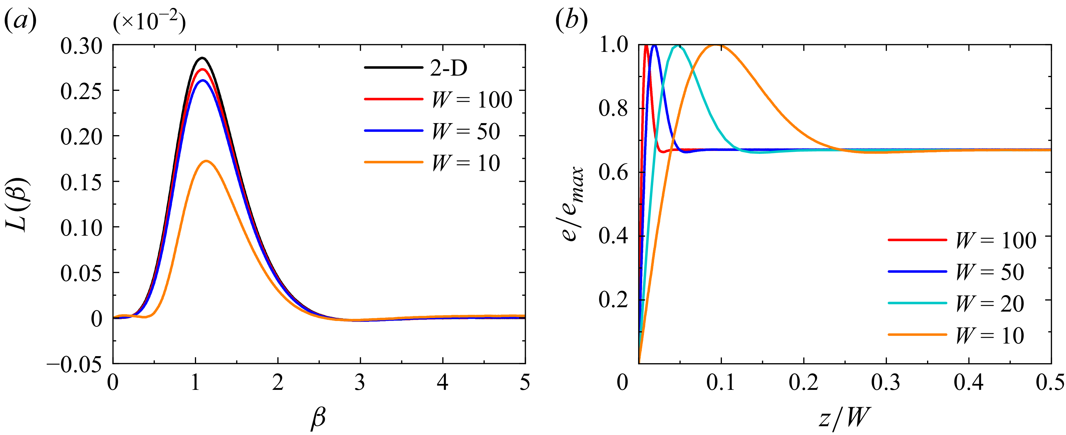
 χ=1
 Re=10
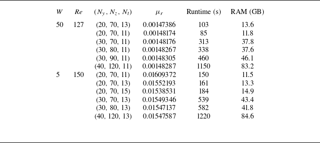
 We=20
 χ=1
 k=1.21
 β=3.5
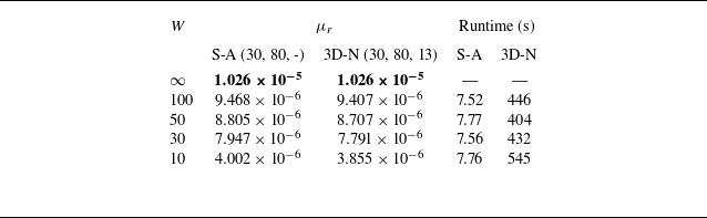
 μr
 β=2
 Re=10
 k=0.001

 β=2
 Re=10
 We=20
 χ=1
 k=0.2
 k
 μr=k2μ2,r
 +

 Rec
 β
 kc
 W
 W=50
 W=10
 W=5
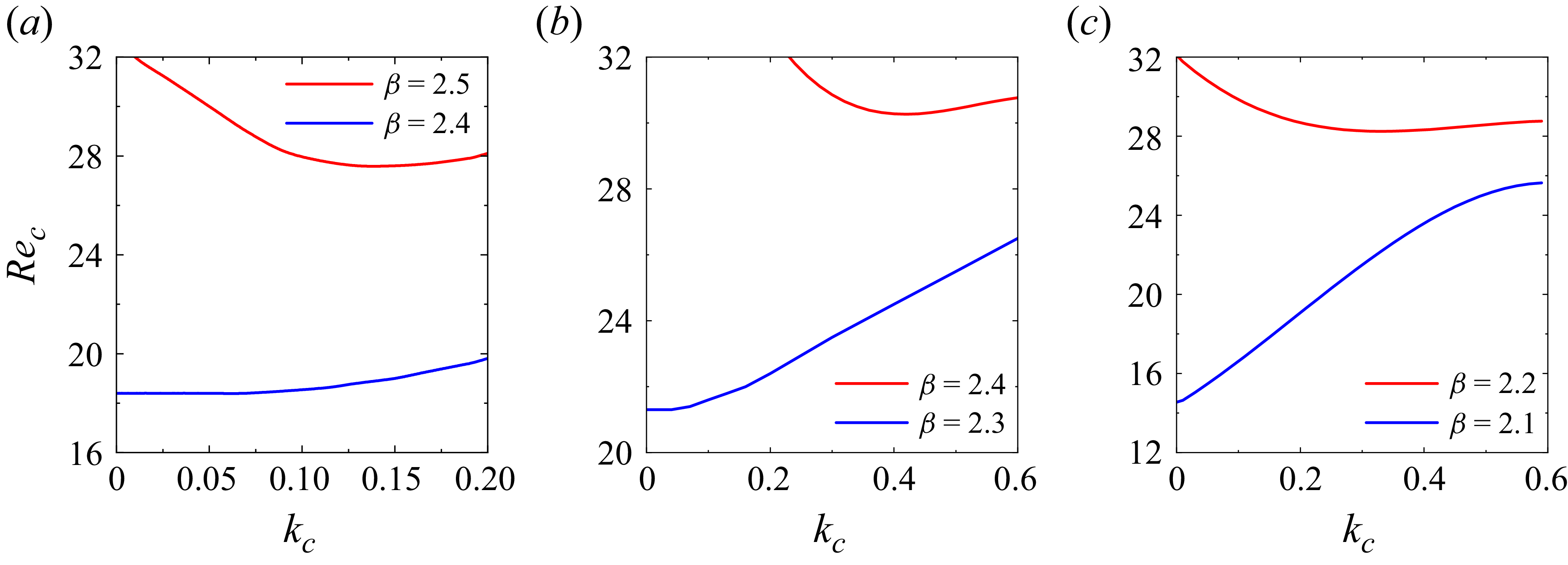
 P2
 P5
 P8

 W
 y=1
 β=2
 Re=10
 k=0.01

 W
 y=1
 β=3.5
 Re=127
 k=1.21

 e=(1/2)(u~2+v~2+w~2)
 e/emax
 x=0
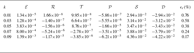
 β=1
 Re=10
 W=50
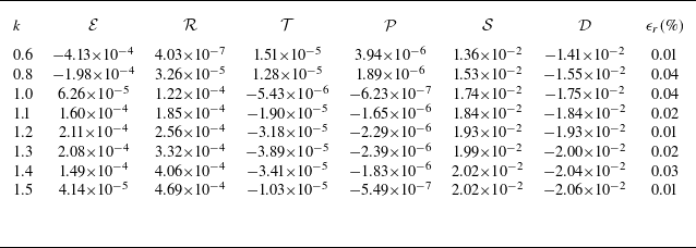
 β=3.5
 Re=130
 W=50
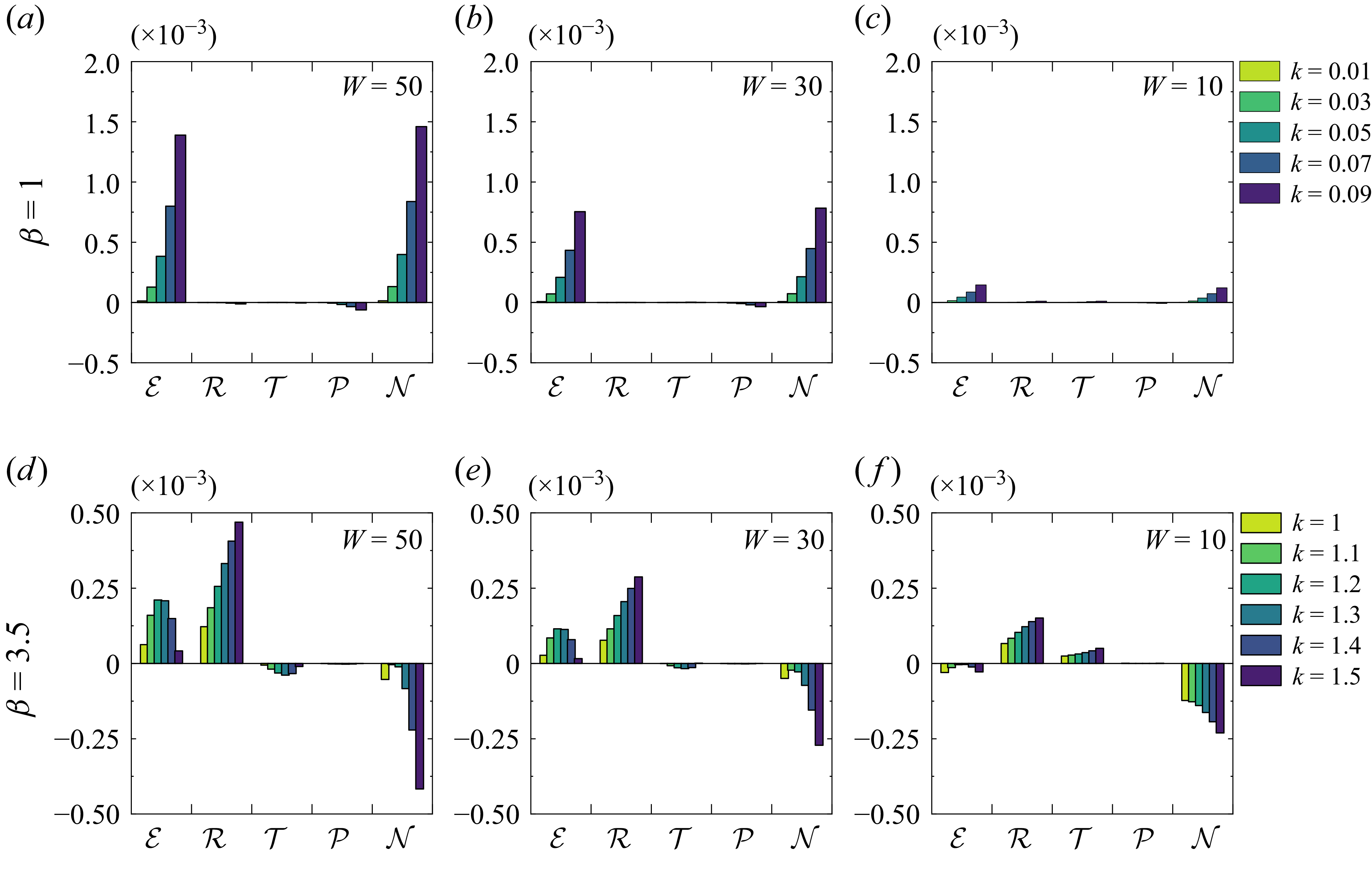
 W
 β=1,Re=10
 β=3.5,Re=130


