2 Self-similar vortex filament structure

Consider a space curve $\boldsymbol{r}(s,t)$ where $s\in \mathbb{R}$ is the arclength variable while $t\geqslant 0$ is time. Then, $\boldsymbol{r}(s,t)$ gives a vortex filament solution provided that it satisfies the non-local dynamics given by (1.1). Since $\unicode[STIX]{x1D705}>0$ , we can scale the time variable like $t=2\unicode[STIX]{x03C0}\hat{t}/\unicode[STIX]{x1D705}$ (leaving only a factor of $1/2$ multiplying the integral in (1.1)). Let us consider a solution $\boldsymbol{r}(s,t)$ with the self-similar structure $\boldsymbol{r}(s,t)=\hat{t}^{a}\boldsymbol{R}(\unicode[STIX]{x1D702})$ where $\unicode[STIX]{x1D702}=s\hat{t}^{b}$ . While such solutions are known to exist for $a=1/2$ and $b=-1/2$ in the case of the LIA (Lipniacki Reference Lipniacki2000, Reference Lipniacki2003a ,Reference Lipniacki b ; Bewley et al. Reference Bewley, Paoletti, Sreenivasan and Lathrop2008; Van Gorder Reference Van Gorder2013), it is not clear exactly what the scalings should be for the non-local equation (1.1). Placing this solution form into (1.1), we obtain

where prime denotes differentiation with respect to the similarity variable $\unicode[STIX]{x1D702}$ and $\hat{\ell }$ denotes the scaled vortex filament in the similarity frame of reference. Clearly, we must have $a=1/2$ , which is the same as for the LIA. Unlike in the LIA, the scaling parameter $b$ is not specified from the equation. However, note that a line filament should be a solution to both the LIA and Biot–Savart dynamics. If we want a line in the self-similar coordinates to correspond with a line in the arclength coordinates, we should have $s=\hat{t}^{1/2}\unicode[STIX]{x1D702}=\hat{t}^{1/2+b}s$ , meaning $b=-1/2$ . Therefore, although the choice of $b=-1/2$ is not forced by the governing equation (as is the case for the LIA), we still find it convenient to make this selection so that line filaments in the self-similar frame map to line filaments in the arclength frame. With this, the governing equation in the self-similar frame becomes

There are two types of vortex filament solutions one might expect from (2.2). The first of these, open vortex filaments, consist of a non-intersecting curve of infinite length in $\mathbb{R}^{3}$ . In § 3 we consider the asymptotics of such solutions under this self-similar formulation. We are able to show that the obtained solutions are in qualitative agreement with self-similar solutions previously obtained under the LIA model. The second type of solution would be closed vortex filaments, consisting of finite length closed curves in $\mathbb{R}^{3}$ . Such solutions would model vortex rings, knotted vortex filaments, and so on. In § 4 we consider the question of whether any such closed vortex filament solutions can exhibit self-similarity.

3 Asymptotics for the open self-similar vortex filament

Let us first consider an open vortex filament, which is a filament of infinite length that does not reconnect or self-intersect. Many vortex filaments studied in the literature, including helices, planar filaments and self-similar filaments, fall into this category. For such a case, the arclength parameter takes all real values, meaning that the integration over $\hat{\ell }$ is equivalent to a parametric integration over the real line. Taking note of this, and then writing the vector $\boldsymbol{R}(\unicode[STIX]{x1D702})=(x(\unicode[STIX]{x1D702}),y(\unicode[STIX]{x1D702}),z(\unicode[STIX]{x1D702}))$ , we can write the coupled integro–differential equations for each of the scalar components in (2.2) as

From the system (3.1)–(3.3), it is clear to see that a line filament $\boldsymbol{R}(\unicode[STIX]{x1D702})=(c_{1}\unicode[STIX]{x1D702},c_{2}\unicode[STIX]{x1D702},c_{3}\unicode[STIX]{x1D702})$ is always a solution, and this immediately gives the line filament $\boldsymbol{r}(s,t)=(c_{1}s,c_{2}s,c_{3}s)$ in arclength coordinates. Many of the self-similar open filament solutions to the LIA in the literature are for Kelvin wave-type structures along line filaments, and these can be realized as small perturbations of the line filament. One typically selects a single coordinate along which to orient the filament curve, and without loss of generality (due to the symmetry of (3.1)–(3.3)) we shall select the $x$ coordinate. Let us take $\unicode[STIX]{x1D716}>0$ to be a small-amplitude parameter, which measures the small deviations of the waves along a line filament. Consider then a solution of the form

We shall consider solutions with $X$ , $Y$ and $Z$ that are of $O(1)$ in epsilon to ensure that the perturbations remain valid. Terms that are of $O(\unicode[STIX]{x1D716}^{3})$ and smaller shall be neglected, since it is physically reasonable to take the amplitude of the perturbations $0<\unicode[STIX]{x1D716}\ll 1$ . Placing (3.4) into (3.1)–(3.3), we obtain

Note that (3.6)–(3.7) decouple from the function $X(\unicode[STIX]{x1D702})$ . Meanwhile, (3.5) has an integral term involving $Y(\unicode[STIX]{x1D702})$ and $Z(\unicode[STIX]{x1D702})$ alone. Therefore, one may solve the two equations (3.6)–(3.7) for $Y(\unicode[STIX]{x1D702})$ and $Z(\unicode[STIX]{x1D702})$ and then substitute the solution into (3.5) to obtain $X(\unicode[STIX]{x1D702})$ .

In order to find the solution pair to (3.6)–(3.7), we shall exploit the symmetry of the equations. Multiplying (3.7) by $\text{i}$ ( $\text{i}=\sqrt{-1}$ ) and adding the two equations, we obtain an equation of the form

where $\unicode[STIX]{x1D6F7}(\unicode[STIX]{x1D702})=Y(\unicode[STIX]{x1D702})+\text{i}Z(\unicode[STIX]{x1D702})$ is a complex-valued function. Once $\unicode[STIX]{x1D6F7}(\unicode[STIX]{x1D702})$ is found, we can recover the desired quantities by noting $Y(\unicode[STIX]{x1D702})=\text{Re}[\unicode[STIX]{x1D6F7}(\unicode[STIX]{x1D702})]$ and $Z(\unicode[STIX]{x1D702})=\text{Im}[\unicode[STIX]{x1D6F7}(\unicode[STIX]{x1D702})]$ .

While the integration in (3.8) is over the real line, in principle the vortex filament is a very thin hollow tube, so there is a small core radius around each point, $|\unicode[STIX]{x1D702}-\hat{\unicode[STIX]{x1D702}}|<\unicode[STIX]{x1D6FF}$ with $\unicode[STIX]{x1D6FF}>0$ , within which the integral does not apply. We assume that $\unicode[STIX]{x1D6FF}\ll \unicode[STIX]{x1D716}\ll 1$ , which is consistent with waves along the filament having much larger amplitudes than the vortex core radius, as is common in experiments and indeed assuming in the framework of the model. Removing this small region from the integral, and merging the integrals over $-\infty <\hat{\unicode[STIX]{x1D702}}<-\unicode[STIX]{x1D6FF}$ and $\unicode[STIX]{x1D6FF}<\hat{\unicode[STIX]{x1D702}}<\infty$ , we obtain

which leaves us with the equation

In the core region, $|\unicode[STIX]{x1D702}-\hat{\unicode[STIX]{x1D702}}|<\unicode[STIX]{x1D6FF}$ , we have regularized by using the LIA (neglecting $O(\unicode[STIX]{x1D716}^{2})$ terms that would give $O(\unicode[STIX]{x1D716}^{3})$ corrections). This regularization method has been suggested and used in numerical studies of superfluid vortex filament dynamics (Schwarz Reference Schwarz1985; Adachi et al. Reference Adachi, Fujiyama and Tsubota2010), and the appeal of this method is that it permits one to directly compare the LIA solutions with the Biot–Savart solutions. This regularization was recently employed to study helical filaments under (1.1) by Van Gorder (Reference Van Gorder2015b ), where the results were used to directly compare the Biot–Savart and LIA solutions. It was also used to regularize the planar filaments of Van Gorder (Reference Van Gorder2015c ).

Let us make an observation. In the case where the integral is approximated by LIA, the integral term goes like $\unicode[STIX]{x1D6F7}^{\prime \prime }$ which gives an equation $\unicode[STIX]{x1D6F7}-\unicode[STIX]{x1D702}\unicode[STIX]{x1D6F7}^{\prime }\sim -\text{i}\unicode[STIX]{x1D6F7}^{\prime \prime }$ . This equation has solutions of the form $\unicode[STIX]{x1D6F7}(\unicode[STIX]{x1D702})\sim c_{1}\unicode[STIX]{x1D702}+c_{2}\unicode[STIX]{x1D702}\unicode[STIX]{x1D719}(\unicode[STIX]{x1D702})$ , where $\unicode[STIX]{x1D719}(\unicode[STIX]{x1D702})$ satisfies $-\unicode[STIX]{x1D702}^{2}\unicode[STIX]{x1D719}^{\prime }=-\text{i}(2\unicode[STIX]{x1D719}^{\prime }+\unicode[STIX]{x1D702}\unicode[STIX]{x1D719}^{\prime \prime })$ . This implies $\unicode[STIX]{x1D719}^{\prime }(\unicode[STIX]{x1D702})$ is of the form $\unicode[STIX]{x1D719}^{\prime }(\unicode[STIX]{x1D702})\sim \unicode[STIX]{x1D702}^{-2}\exp (-(\text{i}/2)\unicode[STIX]{x1D702}^{2})$ . Separating into real and imaginary parts and integrating, one recovers $\unicode[STIX]{x1D6F7}(\unicode[STIX]{x1D702})$ . Such a solution is possible as the small-amplitude perturbations along the filament are effectively linear waves (plus negligibly small nonlinear contributions). Notice that while more complicated, (3.10) is linear in $\unicode[STIX]{x1D6F7}(\unicode[STIX]{x1D702})$ . Therefore, a similar approach may work in the present case, as well. Since we are concerned with small perturbations along a filament which is directed along the $x(\unicode[STIX]{x1D702})$ component, and since amplitude scalings at this order are negligible (since (3.10) is linear in $\unicode[STIX]{x1D6F7}(\unicode[STIX]{x1D702})$ ), we will assume a solution of the form

where $\unicode[STIX]{x1D70C}$ is a parameter to be determined. Note that the other linearly independent solution, $\unicode[STIX]{x1D6F7}(\unicode[STIX]{x1D702})=\unicode[STIX]{x1D702}$ , is neglected, as it would just result in a $O(\unicode[STIX]{x1D716})$ pivot in the $O(1)$ line filament. We would then simply reorient the coordinate frame to remove this pivot. Placing (3.11) into (3.10), we obtain the algebraic relation

The first term on the right-hand side is the LIA contribution from the core, while the second term is the non-local contribution from the outer region. The parameter $\unicode[STIX]{x1D6FE}$ is the Euler–Mascheroni constant ( $\unicode[STIX]{x1D6FE}\approx 0.5772$ ). Since $\unicode[STIX]{x1D6FF}\ll 1$ , we neglect $O(\unicode[STIX]{x1D6FF}^{2})$ contributions from the integral. We therefore find

Compare this to the pure LIA result, which would give $\unicode[STIX]{x1D70C}=-1/(2|\text{ln}(\unicode[STIX]{x1D6FF})|)$ , about double the value of (3.13), where non-local effects are included. Hence, non-locality is expected to modify the spatial scaling of these solutions, while the general qualitative properties should be consistent between the LIA and the Biot–Savart formulations.

Since $\unicode[STIX]{x1D6FF}\ll 1$ , $\ln (\unicode[STIX]{x1D6FF})<0$ and $\unicode[STIX]{x1D70C}<0$ , and hence the expression (3.13) gives $\unicode[STIX]{x1D6F7}(\unicode[STIX]{x1D702})=\unicode[STIX]{x1D702}\int _{0}^{\unicode[STIX]{x1D702}}\unicode[STIX]{x1D70E}^{-2}\exp (-\text{i}|\unicode[STIX]{x1D70C}|\unicode[STIX]{x1D70E}^{2})\,\text{d}\unicode[STIX]{x1D70E}$ . One can separate this into real and imaginary parts and perform the integration, recovering $Y(\unicode[STIX]{x1D702})=\text{Re}[\unicode[STIX]{x1D6F7}(\unicode[STIX]{x1D702})]=-\text{cos}(|\unicode[STIX]{x1D70C}|\unicode[STIX]{x1D702}^{2})-\sqrt{2\unicode[STIX]{x03C0}|\unicode[STIX]{x1D70C}|}\unicode[STIX]{x1D702}S(\sqrt{2|\unicode[STIX]{x1D70C}|/\unicode[STIX]{x03C0}}\unicode[STIX]{x1D702})$ and $Z(\unicode[STIX]{x1D702})=\text{Im}[\unicode[STIX]{x1D6F7}(\unicode[STIX]{x1D702})]=\sin (|\unicode[STIX]{x1D70C}|\unicode[STIX]{x1D702}^{2})-\sqrt{2\unicode[STIX]{x03C0}|\unicode[STIX]{x1D70C}|}\unicode[STIX]{x1D702}C(\sqrt{2|\unicode[STIX]{x1D70C}|/\unicode[STIX]{x03C0}}\unicode[STIX]{x1D702})$ . The functions $S$ and $C$ denote the Fresnel $S$ and $C$ functions, respectively.

From regularization of the integral in (3.5), and using our complex function $\unicode[STIX]{x1D6F7}(\unicode[STIX]{x1D702})$ as found above, we can write the integral as a function of $\unicode[STIX]{x1D702}$ , obtaining

From the form of $M$ defined in (3.14), we have $M(\unicode[STIX]{x1D702};\unicode[STIX]{x1D6FF})=\unicode[STIX]{x1D716}^{2}\tilde{M}(\unicode[STIX]{x1D702};\unicode[STIX]{x1D6FF})$ for $\tilde{M}=O(1)$ in $\unicode[STIX]{x1D716}$ . Note that the integral in (3.14) is purely imaginary, therefore $\tilde{M}(\unicode[STIX]{x1D702};\unicode[STIX]{x1D6FF})$ is a real-valued function. In order to solve for $X(\unicode[STIX]{x1D702})$ from (3.5), note that (3.5) is equivalent to

and manipulating and then integrating (3.15) we obtain

where $X_{0}>0$ is an arbitrary constant of integration and $\unicode[STIX]{x1D702}_{0}$ is some arbitrary value of $\unicode[STIX]{x1D702}$ corresponding to the lower bound of integration. Isolating (3.16) for $X(\unicode[STIX]{x1D702})$ , we have

With this, we have obtained the needed functions to describe the self-similar propagation of waves along a vortex filament up to order $O(\unicode[STIX]{x1D716}^{2})$ contributions, where $\unicode[STIX]{x1D716}$ is the amplitude of the small wave-like perturbations. Mapping the above analysis into the original coordinate frame, the solution which consists of small-amplitude Kelvin waves along a vortex filament is given by

This solution suggests several interesting things. First, self-similar solutions are indeed possible under the non-local Biot–Savart dynamics, and they have been shown here assuming small perturbations of a line filament. The dynamics is accurate to $O(\unicode[STIX]{x1D716}^{2})$ at small amplitude $0<\unicode[STIX]{x1D716}\ll 1$ . Second, the structure of such self-similar solutions is essentially the same as seen under the LIA. Indeed, for small-amplitude perturbations, inclusion of the non-local term (instead of approximating it with LIA) gives a spatial scaling of the aforementioned LIA similarity solutions. That is, $\boldsymbol{r}(s,t)=\boldsymbol{r}_{LIA}(\tilde{s},\tilde{t})$ , where $\boldsymbol{r}_{LIA}$ is the corresponding solution under LIA, $\tilde{s}$ is a scaling of the arclength variable $s$ and $\tilde{t}$ is a scaling of time, $t$ . Third, while it has been known for some time that the helical filament exists under both the non-local Biot–Savart formulation and the LIA (see Van Gorder (Reference Van Gorder2015b ) and references therein), and recently it was shown that planar filaments exist under the Biot–Savart formulation (Van Gorder Reference Van Gorder2015c ), it has never been shown that similarity solutions exist under the Biot–Savart formulation. Unlike in the helical case, where tightly coiled helix solutions exist under the Biot–Savart formulation yet are not accurately reproduced under the LIA, here the self-similar vortex filament structure is qualitatively similar under both Biot–Savart and LIA formulations. This is a feature which is shared with the planar vortex filament, which qualitatively is the same under both non-local and local formulations (with only minor differences in scaling of the space and temporal variables).

Putting (3.18) into Cartesian coordinates instead of arclength, we have that the filament position curve can we written in terms of the single spatial variable, $x$ , and time, $t$ , like

In the $y$ and $z$ components, we have used the scalings

in order to simplify the representations. Observe that, if we had instead neglected integral terms and kept only the inner terms, we would have recovered the LIA solution, which in our notation would be given by

Note the appearance of a scaling parameter, $\unicode[STIX]{x1D707}=\unicode[STIX]{x1D707}(\unicode[STIX]{x1D6FF})$ , which is defined by

for $0<\unicode[STIX]{x1D6FF}\ll 1$ . Variations in the LIA filament curve are therefore more tightly centred around the origin, as the $y$ and $z$ components of the filament, which give the waves, scale as a dilation of the Biot–Savart solution. In particular, $y_{LIA}(x,t)=y_{BS}(\unicode[STIX]{x1D707}x,t)$ and $z_{LIA}(x,t)=z_{BS}(\unicode[STIX]{x1D707}x,t)$ for $\unicode[STIX]{x1D707}>\sqrt{2}$ . Since the LIA dynamics is scaled toward the origin, for any fixed behaviour of the Biot–Savart solution on a spatial interval $[-L,L]$ , the same dynamics is contained in an open spatial interval $(-L/\sqrt{2},L/\sqrt{2})$ when we go to the LIA solutions. Therefore, the Biot–Savart dynamics is more smooth than the LIA dynamics. This makes sense, as the integral in the Biot–Savart dynamics results in a smoothing of solutions when compared to the LIA (which only involves differentiation).

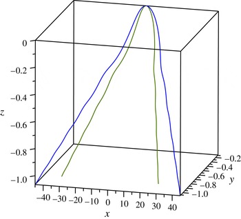
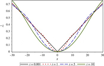
In figure 1, we compare the Biot–Savart solutions (3.19) with the LIA solutions (3.21). Any kinks that form at the centre will necessarily be more sharp under LIA than for the Biot–Savart formulation, due to the scaling property discussed above. In figure 2, we observe the temporal dynamics of a self-similar vortex filament under the Biot–Savart law. As time progresses, the Kelvin waves radiate outward along the vortex filament, resulting in a smoothing of the structure. Conversely, one observes very sharp kinks in the singular limit $t\rightarrow 0^{+}$ . These kinks are smoothed as the central region sheds Kelvin waves.

Figure 1.

Comparison of the regularized Biot–Savart (blue curve) and LIA (green curve) vortex filament solutions given by (3.19) and (3.21), respectively. Parameter values are $\unicode[STIX]{x1D716}=0.1$ , $\unicode[STIX]{x1D6FF}=0.001$ , while the plots are given at time $\hat{t}=2$ . While qualitatively similar, the LIA filament has a sharper kink at the origin. As suggested by the scaling ratio satisfying $\unicode[STIX]{x1D707}>2$ , we have that the LIA solutions will have sharper kinks at the origin than the corresponding Biot–Savart solutions.

Figure 2.

Time evolution of a regularized Biot–Savart vortex filament solutions given by (3.19). Parameter values are $\unicode[STIX]{x1D716}=0.1$ , $\unicode[STIX]{x1D6FF}=0.001$ , while we sample a variety of times. For ease of viewing, we plot solutions in the $(x,-z)$ plane. As time increases, the sharp kink at the origin is smoothed, while the filament radiates Kelvin waves radially outward from this kink. Note that we have picked the scaling parameter to be $X_{0}=1$ . For other values, we may make the kink at the origin more or less sharp at $t=0$ , with the structure being smoothed as $t$ increases.

While the angle of the kinks located at the origin shown in figures 1 and 2 appear rather obtuse, this is due to the choice of spatial scaling, since $X_{0}=1$ in those plots. If this scaling factor is decreased, the angle formed decreases, and vice versa. Meanwhile, if $\unicode[STIX]{x1D716}$ is increase, the angle formed decreases. While the analytical theory outlined here is valid for sufficiently small $\unicode[STIX]{x1D716}$ , a similar trend should be observed in any numerical simulations (provided again that the scaling factor is chosen appropriately). The core parameter, $\unicode[STIX]{x1D6FF}$ , is taken to be less than $\unicode[STIX]{x1D716}$ for physical reasons, although changes are apparent even for small changes in $\unicode[STIX]{x1D6FF}$ . 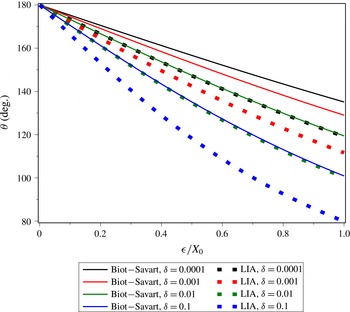These results are demonstrated in figure 3.

Figure 3.

Comparison of the interior angle $\unicode[STIX]{x1D703}$ in the kink solutions near the origin for small time under both Biot–Savart (3.23) and LIA (3.24) models. We plot the angles over the ratio $\unicode[STIX]{x1D716}/X_{0}$ , which is the ratio of the deflection extent to the spatial scaling, as this ratio is what enters into the analytical formulas (3.23) and (3.24). As the ratio increases (that is, as the spatial scaling becomes compatible with the deflection size), the kink in the filament at $t=0$ becomes more sharp. Furthermore, the role of the core radius parameter, $\unicode[STIX]{x1D6FF}$ , is to make this kink more sharp. This means that the thicker the filament, the more obtuse the angle will tend to be. Note also that the LIA solutions result in uniformly more share kinks in all cases. This makes sense, in light of the fact that the non-local integral part of the Biot–Savart dynamics was suggested to have a smoothing effect on the solutions. However, these plots make it clear that the smoothing effects do not modify the qualitative features of self-similar solutions previously observed under the LIA.

In order to analytically calculate the angles formed for very small $t$ , as shown in figure 3, we took the $t\rightarrow 0$ limit of the approximate solution (3.19). This limit resulted in two rays emanating from the origin, one corresponding to $x>0$ , the other corresponding to $x<0$ . From standard vector calculus, the angle between these two (which corresponds to the angle of the kink seen in figures 1 and 2 for very small time), is given by

in units of degrees. A corresponding result for the angle formed at the origin by the kink in the LIA solutions (3.21) is found to be

We find that wider filaments (corresponding to larger values of $\unicode[STIX]{x1D6FF}$ ) result in sharper kinks, and hence appear to have less regularity. As the ratio $\unicode[STIX]{x1D716}/X_{0}$ increases, the kinks will become sharper. Thus, solutions with larger spatial deflections or more rapid spatial variation can have sharper kinks for small time. Note that the results plotted in figure 3 correspond to the $t\rightarrow 0$ limit. When $t$ increases, the kink initially at the origin will smooth in all cases, as the kink radiates Kelvin waves; this dynamics was seen in figure 2 for the Biot–Savart case, and holds true for other parameter values (as well as for the corresponding LIA solutions). When comparing the Biot–Savart solutions with the LIA solutions, note that the LIA solutions result in sharper initial kinks given the same parameter values. This is in agreement with the view that the Biot–Savart dynamics smooth the filament structures. Still, the dynamics emergent for each of the Biot–Savart and LIA models are in complete qualitative agreement, suggesting that the self-similar structures observed in the literature under the LIA are likely valid under more complicated (and more computationally involved) Biot–Savart dynamics.

4 On the existence of a self-similar closed vortex filament

A closed vortex filament is a vortex filament of finite length which closes on itself (one may connect one end of an open filament of finite length to the other in order to close the filament curve). The primary example of such a filament is a curve corresponding to a thin vortex ring. The parameterization with arclength can therefore be viewed as periodic, say $0<s<2\unicode[STIX]{x03C0}$ , and this gives the bounds for the integration over $\ell$ . Now, for the parameterization with $\unicode[STIX]{x1D702}$ , since the arclength is bounded the end points are in general time dependent. Therefore, the integration over $\hat{\ell }$ will take place on the interval $0<\unicode[STIX]{x1D702}<(2\unicode[STIX]{x03C0}/\sqrt{\hat{t}})$ . This temporal upper bound is undesirable for multiple reasons. First, this explicit time dependence means that there is not true similarity in the solution. Second, as time increases, the size of the closed filament tends to zero, even if the size is static in the arclength frame. Finally, as time is taken to zero, the length in the new coordinate becomes infinite. For these reasons, the type of similarity transform used above is not particularly helpful for studying closed filaments.

We would like a solution which would maintain the length parameterization of the closed curve. Recall that we picked the similarity parameter $b=-1/2$ so that line filaments would be mapped to line filaments. As line filaments are never closed curves, we should not be concerned with this here. Therefore, it makes more sense to pick $b$ in order to maintain the structure of the closed curve solutions for all time. For this reason, we pick $b=0$ . This gives $\unicode[STIX]{x1D702}=s$ , and the solution structure is $\boldsymbol{r}(s,t)=\sqrt{\hat{t}}\boldsymbol{R}(\unicode[STIX]{x1D702})=\sqrt{\hat{t}}\boldsymbol{S}(s)$ , where $\boldsymbol{S}(s)$ is a curve depending on arclength alone. The spatial structure of the curve can be found from solving

where again $s\in \mathbb{R}$ denotes arclength. Yet, since $\boldsymbol{S}$ depends only on arclength, this means $\boldsymbol{r}(s,t)$ is a static curve in space which is scaled by time in a multiplicative manner. At time $t=0$ , the curve will emanate from a point $\boldsymbol{r}(s,0)=(0,0,0)$ and as time progresses one will have a curve of the form $\boldsymbol{r}(s,t)=(\sqrt{\hat{t}}x(s),\sqrt{\hat{t}}y(s),\sqrt{\hat{t}}z(s))$ which maintains form but undergoes dilation as it expands in space. As time becomes infinitely large, the curve will enclose an infinite region. This behaviour is the opposite of the type of behaviour seen when we instead had taken $b=-1/2$ . Therefore, each respective scaling will give a closed filament of infinite length for large ( $b=0$ ) or small ( $b=-1/2$ ) time, with contraction (dissipation) of the closed filament in the respective opposite temporal limits. We find that the $b=0$ behaviour is representative of $b\geqslant 0$ , while the $b=-1/2$ behaviour is representative of $b<0$ , hence the two types of behaviours given above are the only possible behaviours for self-similar closed filaments. Interestingly, this means that behaviours observed near core overlapping events during the collapse of vortex rings by Fernandez et al. (Reference Fernandez, Zabusky and Gryanik1995) could not be sustained, and hence should only be observed in the small time limit. Rather, such a dynamics could be viewed as perturbations to some self-similar process, with the perturbations dominating away from the core overlapping if one were to consider the time reversal of the process. We should point out the collapse of a vortex filament to a point singularity in a manner consistent with a self-similarity scaling $(t-t_{0})^{1/2}$ was described in Siggia (Reference Siggia1985). In that study, Siggia used a modified Biot–Savart formulation in order to numerically simulate results. Note that a time reversal would then allow one to generate a filament of infinite length from a point singularity.

Ricca, Samuels & Barenghi (Reference Ricca, Samuels and Barenghi1999) considered perturbations of closed circular vortex filaments in order to study vortex knots under the Biot–Savart dynamics. One may wonder if such solutions satisfy a similarity scaling. As we’ve shown here, one needs $b=0$ for a self-similar closed filament. However, if we assume such a solution, and then place it into (4.1), we find that no circular curve can be a solution (no matter the choice of orientation, or parameters used such as the radius). As the results of Ricca et al. (Reference Ricca, Samuels and Barenghi1999) were obtained from perturbations about circular curves, it is clear that such solutions would not likely satisfy (4.1) after translation or parameter scaling. Therefore, we would not expect closed curves corresponding to vortex circular rings, not more complicated knotted filaments, to exhibit self-similarity.

We should also note that more general planar solutions than even circular solutions will not exist for (4.1). To show this, note that a planar solution can be written with two components without loss of generality, as one may always rotate the coordinate frame. Taking $\boldsymbol{S}(s)=(A(s),B(s),0)$ such that $A$ and $B$ are $2\unicode[STIX]{x03C0}$ -periodic, we find that (4.1) gives

Therefore, for the planar case, the left- and right-hand sides of (4.1) are orthogonal to one another, and the only solution is the trivial solution $A=0$ and $B=0$ . Hence, no planar solution exists.

In order to get a better feeling for whether a solution to (4.1) may actually exist, let us close this section by noting that for many filaments, there is some parameter limit where Biot–Savart dynamics agrees at least qualitatively with that found under the LIA. We demonstrated this in the previous section for open filaments, and this is true of other types of solutions, such as helical filaments (when the filament is not tightly coiled; see Van Gorder (Reference Van Gorder2015b )) and planar filaments (Van Gorder Reference Van Gorder2015c ). Therefore, to get an understanding of the qualitative features of a solution to (4.1), let us consider a relevant LIA approximation. Assuming the spatial variable $s$ is scaled appropriately, we may ignore the factor arising under LIA, and simply approximate (4.1) by

where prime denotes differentiation with respect to $s$ . Differentiation with respect to $s$ yields

which implies that either the right-hand side is orthogonal to the left-hand side (which makes no sense) or that $\boldsymbol{S}^{\prime }=\mathbf{0}$ . Since only the latter case is possible, we must have that $\boldsymbol{S}(s)=\boldsymbol{S}^{0}$ , a constant vector. Yet, the only constant solution to (4.3) is the zero solution. We have therefore shown that there exist no non-trivial solutions to (4.3). Then, in the case where the LIA and Biot–Savart solutions agree, there would exist no non-trivial solution to (4.1), meaning there would exist no closed self-similar vortex filament. Now, it may be that there could arise some pathological case which permits a non-trivial solution of (4.1) which does not correspond to a solution of (4.3). Hence, we suggest only that it is unlikely that a non-trivial solution to (4.1) exists, and we have no proof for the general Biot–Savart dynamics. It is therefore an open question whether a bounded and periodic solution actually exists for (4.1). Even if such a solution were to exist, it would maintain its form while growing like $\sqrt{t}$ as $t$ increases. Such a solution may not be physical.