1. Introduction
There has been a long-standing scientific interest in gravity–capillary waves (commonly referred to as wind ripples, see Zhang Reference Zhang1995), due to their importance in the exchange of momentum, thermal energy and gases between the ocean and the atmosphere. Furthermore, wind ripples are of theoretical interest, as they occur at the scale set when the restoring forces due to gravitation and surface tension are equally important, and therefore give rise to a new type of solitary wave. In contrast to the pure gravity solitary waves in shallow water, gravity–capillary solitary waves can exist on the surface of both two- and three-dimensional fluids and at arbitrary depth. When the Bond number
 $B={\it\sigma}/{\it\rho}gh^{2}$
(
 ${\it\sigma}$
is the surface tension coefficient,
 ${\it\rho}$
is the fluid density,
 $g$
is the gravitational acceleration and
 $h$
is the depth of the fluid) is less than
 ${\textstyle \frac{1}{3}}$
, these waves resemble wavepackets featuring oscillatory decaying tails; therefore, they are usually called wavepacket solitary waves (Longuet-Higgins Reference Longuet-Higgins1989). The existence of wavepacket solitary waves requires that the phase speed has a global extremum at finite wavenumber, where the group velocity and the phase velocity are equal. Traditionally, at this non-dispersive point, one approximates such wavepackets with a cubic focusing nonlinear Schrödinger equation (NLS) in the modulational regime, where the sech-type soliton solution of the stationary NLS approximates the envelope of the solitary waves in the primitive equation.
The numerical computation of gravity–capillary solitary waves for the irrotational Euler equation has received considerable attention in the past few decades, beginning when Longuet-Higgins (Reference Longuet-Higgins1989) first found a new type of solitary waves in deep water. These ‘depression’ symmetric wavepacket solitary waves have a negative free-surface elevation at their centre. Later, Vanden-Broeck & Dias (Reference Vanden-Broeck and Dias1992) found another branch of solitary waves with a positive free-surface elevation at the centre, which were thereafter called elevation solitary waves. These two branches are both symmetric solitary waves, bifurcating from infinitesimal periodic waves at the minimum of the phase speed, and exist at subcritical speeds.
Unlike the classic gravity solitary waves which can only exist in symmetric form (see Craig & Sternberg (Reference Craig and Sternberg1988) for the rigorous proof), there is some evidence that asymmetric solitary waves may exist in the presence of both gravity and surface tension. Based on theoretical study, asymptotic analysis and numerical computation of the fifth-order Korteweg–de Vries (KdV) equation, a reduced model for small-amplitude gravity–capillary waves of finite depth when the Bond number is close to
 ${\textstyle \frac{1}{3}}$
, a rich structure of symmetric and asymmetric fully localised travelling waves may exist in the water wave problem (see Zufiria (Reference Zufiria1987), Buffoni, Champneys & Toland (Reference Buffoni, Champneys and Toland1996), Champneys & Groves (Reference Champneys and Groves1997), Yang & Akylas (Reference Yang and Akylas1997) and the references therein). In particular, Yang & Akylas (Reference Yang and Akylas1997) showed that the two symmetric elevation and depression branches are the only ones that can bifurcate from infinitesimal periodic waves at the minimum speed of linear waves, and that close to the bifurcation point their envelopes are governed by single-hump solutions of the NLS. They also showed that, at finite amplitude, there are an infinite number of symmetric and asymmetric solitary-wave branches formed by two or more adjacent packets. Buffoni, Groves & Toland (Reference Buffoni, Groves and Toland1996) used a rigorous centre manifold reduction to show that the plethora of multiple solutions to the fifth-order KdV model equation must persist in the full water wave problem at small amplitude and
 $B={\textstyle \frac{1}{3}}$
. The fifth-order KdV equation remains a restricted model for gravity–capillary waves, only valid when the mean depth of the water is close to 0.5 cm and for small amplitudes (Zufiria Reference Zufiria1987). One can therefore ask the question whether asymmetric solitary waves can be obtained in the full irrotational Euler equations in more realistic situations.
In this paper we focus on the deep-water case which, given the typical wavelength of gravity–capillary waves for an air–water interface, is applicable when the water is deeper than a few centimetres. We shall present numerical evidence of asymmetric gravity–capillary solitary waves on deep water. This is, to the best of our knowledge, the first time that non-symmetric solitary waves have been computed using the irrotational Euler equations. The numerical procedure is outlined in § 2. The main results are presented in § 3, including the typical wave profiles and the bifurcation behaviour. In the conclusions, we discuss possible extensions to the work.
2. Numerical procedure
Consider a two-dimensional irrotational flow of an inviscid incompressible fluid of infinite depth. The flow is bounded above by a free surface. The effects of gravity and surface tension are taken into account. We introduce Cartesian coordinates with
 $y=0$
at the constant level of the free surface at infinity. We denote the equation of the free surface by
 $y={\it\eta}(x,t)$
. We define the velocity potential by
 ${\it\phi}(x,y,t)$
, which satisfies the Laplace equation within the fluid domain, namely,
 ${\it\phi}_{xx}+{\it\phi}_{yy}=0$
for
 $y<{\it\eta}(x,t)$
. Solutions travelling at a constant velocity
 $c$
can be found by assuming that the unknowns
 ${\it\eta}$
and
 ${\it\phi}$
depend on
 $x-ct$
. Therefore the kinematic and dynamic boundary conditions on the free surface
 $y={\it\eta}(x,t)$
can be written as
 $$\begin{eqnarray}\displaystyle & -c{\it\eta}_{x}=-{\it\eta}_{x}{\it\phi}_{x}+{\it\phi}_{y}, & \displaystyle\end{eqnarray}$$
 $$\begin{eqnarray}\displaystyle & \displaystyle -c{\it\phi}_{x}=-\frac{1}{2}\left({\it\phi}_{x}^{2}+{\it\phi}_{y}^{2}\right)-{\it\eta}+\frac{{\it\eta}_{xx}}{(1+{\it\eta}_{x}^{2})^{3/2}}. & \displaystyle\end{eqnarray}$$
 $({\it\sigma}/{\it\rho}g)^{1/2}$
and
 $({\it\sigma}/{\it\rho}g^{3})^{1/4}$
as the units of length and time.
To handle the unknown free surface, we use a conformal transformation, mapping the physical fluid domain to the lower half-plane. The map is defined by
 $z({\it\xi},{\it\zeta})=x({\it\xi},{\it\zeta})+\text{i}y({\it\xi},{\it\zeta})$
with the horizontal and vertical coordinates in the new plane denoted by
 ${\it\xi}$
and
 ${\it\zeta}$
respectively. The free surface is mapped to the
 ${\it\xi}$
-axis, and can therefore be parameterised by
 $Y({\it\xi})\triangleq {\it\eta}(x({\it\xi},0))$
. In the transformed plane, (2.1) and (2.2) can be recast into a single integro-differential equation for
 $Y$
and
 $c$
as unknowns,
 $$\begin{eqnarray}\frac{c^{2}}{2}\left(\frac{1}{X_{{\it\xi}}^{2}+Y_{{\it\xi}}^{2}}-1\right)+Y+\frac{Y_{{\it\xi}}X_{{\it\xi}{\it\xi}}-X_{{\it\xi}}Y_{{\it\xi}{\it\xi}}}{(X_{{\it\xi}}^{2}+Y_{{\it\xi}}^{2})^{3/2}}=0,\end{eqnarray}$$
together with
 $X_{{\it\xi}}=1-\mathscr{H}[Y_{{\it\xi}}]$
, where
 $\mathscr{H}$
is the Hilbert transform defined on the real line
 $\mathbb{R}$
as
 $$\begin{eqnarray}\mathscr{H}[\,f]=\int _{\unicode[STIX]{x211D}}\frac{f({\it\xi}^{\prime })}{{\it\xi}^{\prime }-{\it\xi}}\text{d}{\it\xi}^{\prime }.\end{eqnarray}$$
The detailed derivation of these equations can be found, for example, in Milewski, Vanden-Broeck & Wang (Reference Milewski, Vanden-Broeck and Wang2010) and it is noted that (2.3) is equivalent to the equation obtained in Vanden-Broeck & Dias (Reference Vanden-Broeck and Dias1992) by using the hodograph transformation for a steady solution in a frame moving with the wave.
The energy of the solitary waves will be used as a parameter in the bifurcation curves, and is the sum of the kinetic and potential energies,
 $$\begin{eqnarray}E=\frac{1}{2}\int _{\unicode[STIX]{x211D}}\text{d}x\int _{-\infty }^{{\it\eta}}\left({\it\phi}_{x}^{2}+{\it\phi}_{y}^{2}\right)\text{d}y+\frac{1}{2}\int _{\unicode[STIX]{x211D}}{\it\eta}^{2}\text{d}x+\int _{\unicode[STIX]{x211D}}\left(\sqrt{1+{\it\eta}_{x}^{2}}-1\right)\text{d}x.\end{eqnarray}$$
This can be rewritten in the transformed plane as follows:
 $$\begin{eqnarray}E=\frac{1}{2}\int _{\unicode[STIX]{x211D}}\left[c^{2}Y_{{\it\xi}}\mathscr{H}[Y]+2\left(\sqrt{X_{{\it\xi}}^{2}+Y_{{\it\xi}}^{2}}-X_{{\it\xi}}\right)+Y^{2}X_{{\it\xi}}\right]\text{d}{\it\xi}.\end{eqnarray}$$
Equation (2.3) is solved numerically by approximating
 $Y$
by the truncated Fourier series
 $$\begin{eqnarray}Y=\mathop{\sum }\limits_{n=-N}^{N}(a_{n}+\text{i}b_{n})\text{e}^{\text{i}2{\rm\pi}n{\it\xi}/L},\end{eqnarray}$$
with
 $b_{0}=0$
, and for
 $n\neq 0$
,
 $a_{-n}=a_{n}$
,
 $b_{-n}=-b_{n}$
. We remark that, for waves symmetric about
 ${\it\xi}=0$
,
 $b_{n}=0$
. Fixing
 $L$
and
 $N$
and
 $c$
, there are
 $2N+1$
unknowns:
 $a_{0},a_{1},\dots ,a_{N},b_{1},b_{2},\dots ,b_{N}$
. These unknowns are required to satisfy the
 $2N+1$
equations obtained by projecting (2.3) onto each element of the basis
 $\text{e}^{\text{i}2{\rm\pi}n{\it\xi}/L}$
for
 $n=0,\dots ,N$
. The nonlinear terms in (2.3) are computed at uniform grid points in
 ${\it\xi}\in [-L/2,L/2)$
whereas the Hilbert transform and derivatives are computed in Fourier space using Fourier multipliers. For example,
 $\widehat{\mathscr{H}[Y]}=\text{i}\,\text{sgn}(k)\widehat{Y}$
, where the hat denotes the Fourier transform and
 $k$
the wavenumber. The equations are solved by Newton iterations and the branches are found by straightforward continuation in a chosen parameter (usually the energy, unless a turning point is reached). This method of solution was successfully implemented in Milewski et al. (Reference Milewski, Vanden-Broeck and Wang2010) for finding symmetric waves that were then used in the time-dependent computations. The computation of asymmetric solitary waves is far more expensive than that of symmetric solutions. Not only do these solutions require double the number of unknown Fourier coefficients, but their multi-packet nature results in a much larger computational domain being needed. The solution was considered to have converged when the
 $L^{\infty }$
-norm of the residual error was less than
 $10^{-11}$
. Various versions of the algorithm were implemented, calculating both the equations and the error in either Fourier or physical space with the same results.
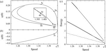
Speed–amplitude and speed–energy curves for symmetric elevation and depression solitary waves emerging from the bifurcation point
 $c^{\ast }=\sqrt{2}$
. (a) The complex behaviour of the speed–amplitude curve for the elevation branch, with the sharp nature of the second turning point shown in more detail. The labelled points correspond to the waves that will be used to construct initial guesses in the remaining figures. (b) The speed–amplitude curve of the depression branch. (c) The energy of the depression branch (dashed line) and of the elevation branch (solid line), showing a zigzag behaviour.

A branch arising from an asymmetric wave with the initial guess being composed of a one-hump elevation wave and a depression wave propagating at
 $c=1.4$
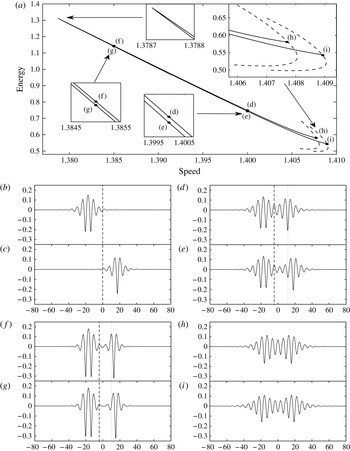
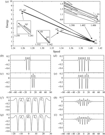
. (a) Speed–energy curves for asymmetric waves (solid line) and symmetric waves (dashed line). The sharp turning point and the symmetry-breaking bifurcations are shown in detail. (b,c) Profiles of the elevation wave labelled 2b in figure 1(a) and the depression wave labelled 2c in figure 1(b). (d–i) Typical profiles marked in (a) with the same labels. (d,e) Typical profiles of asymmetric solitary waves close to the bifurcation points. ( f,g) Typical profiles of asymmetric solitary waves close to the turning point. (h,i) Waves at the symmetry-breaking bifurcation points.

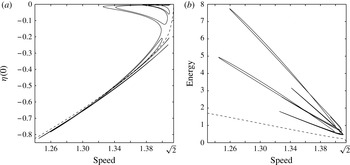
Speed–amplitude and speed–energy curves for a new branch of symmetric depression solitary waves (solid curve), together with the known depression branch (dashed). This branch was found by following asymmetric waves to their original symmetry-breaking bifurcation. (a) The complex behaviour of the speed–amplitude curve for the branch, reminiscent of elevation branches. (b) The energy of the branch, showing the discrete nature of the slope due to the similarity of the waves to a discrete set of single waves placed side-by-side.

A branch arising from an asymmetric wave with the initial guess being composed of two distinct multi-hump elevation solitary waves propagating at
 $c=1.4$
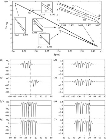
. (a) Speed–energy curves for asymmetric waves (solid line) and symmetric waves (dashed line). The sharp turning points and the symmetry-breaking bifurcations are shown in detail. (d–i) Typical profiles marked in (a) with the same labels. (b,c) Wave profiles labelled 4b and 4c in figure 1(a) respectively. (d,e) Typical profiles of asymmetric solitary waves close to a turning point near
 $c^{\ast }$
. ( f,g) Typical profiles of asymmetric solitary waves close to the turning point at a minimum of
 $c$
. (h,i) Wave profiles at turning points.

A branch arising from an asymmetric wave with the initial guess being composed of a one-hump and a multi-hump elevation solitary wave propagating at
 $c=1.35$
. (a) Speed–energy curves for asymmetric waves (solid line) and symmetric waves (dashed line). The symmetry-breaking bifurcation is shown in detail. (b,c) Wave profiles corresponding to the points labelled 5b and 5c respectively in figure 1(a). (d–i) Typical profiles marked in (a) with the same labels. (d,e) Typical profiles of asymmetric solitary waves at the turning points. ( f,g) Typical profiles of asymmetric solitary waves at the turning point near a minimum of
 $c$
. For ( f)
 ${\it\eta}(P_{1})=0.1104$
,
 ${\it\eta}(Q_{1})=0.1342$
,
 ${\it\eta}(S_{1})=0.1463$
,
 ${\it\eta}(T_{1})=0.1727$
and for (g)
 ${\it\eta}(P_{2})=0.1109$
,
 ${\it\eta}(Q_{2})=0.1618$
,
 ${\it\eta}(S_{2})=0.1471$
,
 ${\it\eta}(T_{2})=0.1743$
. (h,i) The wave profiles at the symmetry-breaking bifurcation points.

Since a long periodic domain is used to approximate solitary waves, the underlying period
 $L$
and the number of mesh points
 $N$
are both chosen sufficiently large so that, to the numerical accuracy we use, the solution does not change when
 $L$
and
 $N$
are increased. This is tested by checking that the residual is less than
 $10^{-11}$
when
 $L$
and
 $N$
are changed. Further details on these parameters are provided in § 3. Overall, the above accuracy was achieved for all the numerical computations when the grid spacing
 ${\rm\Delta}{\it\xi}$
was chosen to be in the range 0.025–0.05.
Two types of symmetric gravity–capillary solitary waves, elevation and depression depending on the height of the free surface at the centre, are known to exist on deep water. The speed–amplitude (where ‘amplitude’ is defined as the centre elevation) and speed–energy bifurcation diagrams of the two branches are presented in figure 1, with typical profiles being shown in figures 2(b,c), 4(b,c) and 5(b,c). The solution branch of depression waves is monotonic in both amplitude and energy (see figure 1
b and the dashed line in figure 1
c) and, as the amplitude increases along the branch, the waves become less oscillatory with a large central depression (contrast figures 2
b and 5
b). The elevation branch exhibits zigzag behaviour (see figure 1
a) first observed in Dias, Menasce & Vanden-Broeck (Reference Dias, Menasce and Vanden-Broeck1996). This behaviour is clear in the speed–energy graph in figure 1(c) (see also figure 3
b): the elevation branch traces back-and-forth, close to lines of slope approximately
 $2s,3s,\dots \,$
, where
 $s$
is the slope of the depression branch. The reason for these slopes is that waves at large amplitude look like several copies of the basic depression wave placed side-by-side.
In order to compute asymmetric solitary waves, it is essential to choose a good initial guess for the Newton iterations. Motived by the analysis of Yang & Akylas (Reference Yang and Akylas1997), we prepare the initial data by superposing two offset symmetric solitary waves with distinct profiles but travelling at the same speed. The zigzag behaviour of the elevation branch gives us more freedom than in Yang & Akylas (Reference Yang and Akylas1997) in preparing the initial data for the Newton iterations because of the many possible choices of elevation waves travelling at the same speed. For example, points 2b, 2c, 4b, 4c in figure 1 are all waves travelling at the same speed.
3. Results
The numerical procedure outlined in the previous section was used to compute branches of asymmetric gravity–capillary solitary waves resulting from different initial guesses. The first numerical experiment presented is shown in figure 2. The initial guess for the Newton iteration was obtained by the simplest combination: a one-hump elevation (figure 2
b corresponding to the point 2b in figure 1
a) superposed with a depression solitary waves (figure 2
c corresponding to the point 2c in figure 1
b), both of which translate at
 $c=1.4$
. The vertical dashed line shown in figures 2(b,c) indicates the points at which these two symmetric solitary waves were glued together. In preparing initial data, we attempted two methods: glueing, whereby the profiles of both waves are cut and connected at the gluing point, and superposition, whereby the waves are linearly superposed after a relative shift. Both methods appear to work equally well.
With the initial guess described above, the algorithm converged to the solution as shown in figure 2(e). This numerical experiment was carried out with
 $L=300$
and
 $N=6000$
. Once this solution was obtained, a global investigation of asymmetric solutions along this branch could be carried out through continuation methods. We found that this new branch begins and ends on branches of symmetric waves. Increasing the speed from point (e), the curve was found to finish on a symmetry-breaking bifurcation point at
 $c=1.4089$
labelled (i) in figure 2(a). Decreasing the speed from point (e), the speed–energy curve experiences a turning point at
 $c=1.3788$
, where the wave speed attains its minimum value. The speed along the branch then increases until it reaches a symmetry-breaking bifurcation point at
 $c=1.4077$
, labelled (h) in figure 2(a). Wave profiles were considered to be symmetric in the non-symmetric formulation if, after choosing a symmetry point that minimises the difference of the solution and its mirror image about that point, the absolute difference between the two is less than
 $10^{-3}$
. The candidate symmetrical solution was then also checked on a code enforcing the symmetry.
The comparison between two different asymmetric solitary waves propagating at the same speed is made in figures 2(d,e) at
 $c=1.4$
and figures 2( f,g) at
 $c=1.385$
. In each of these pairs of figures, to the left of the vertical dashed line, the profiles are almost identical. The vertical dotted line is drawn to indicate the relative horizontal shift between the elevation packet and the depression packet. For example, from (d) to (e) the distance between the two packets has increased by approximately one wavelength of the carrier wave. We can also conclude from these figures that the amplitude is not a suitable parameter to plot the bifurcation curve since the maximum (or the minimum) values of waves propagating at the same speed are almost identical. The profiles according to the two symmetry-breaking bifurcation points are shown in figures 2(h,i) respectively. It should be noted that (i) has an additional wavelength with five troughs between the two minima instead of four in (h). The appearance of these multi-packet symmetric solitary waves had been observed by Buffoni et al. (Reference Buffoni, Champneys and Toland1996) for the fifth-order KdV equation. We have continued the multi-packet symmetric branches (see the dashed lines in a): the branch corresponding to figure 2(h) is in fact connected to the fundamental elevation branch (shown in figure 1), whereas the branch corresponding to figure 2(i) appears to be a new branch of ‘depression’ solitary waves. This branch is shown in figure 3.
We now consider a different branch of asymmetric solitary waves, obtained by piecing together two symmetric multi-hump elevation solitary waves with the same speed, labelled 4b and 4c in figure 1(a). The gluing points are shown in figures 4(b,c) via the vertical dashed line. The Newton algorithm converged to the solution shown in figure 4(d). Using this as the starting point, the complete bifurcation curve could then be followed. This computation was carried out in a domain with
 $L=300$
and
 $N=10\,000$
equally spaced points. The speed–energy curve of asymmetric solitary waves, the solid line shown in figure 4(a), manifests similar zigzag behaviour to that found in other cases. In contrast to figure 2(a), there are multiple turning points occurring both at large amplitude and close to the critical speed
 $c^{\ast }$
. The fate of this bifurcation curve is the same as that of figure 2, namely that the non-symmetric branch connects the two symmetry-breaking bifurcations (dashed curves in figure 4
a) on branches of symmetric waves.
Typical wave profiles are presented in figures 4(d–i). First, waves on both sides of a turning point close to
 $c^{\ast }$
are shown in (d,e). It should be noted that the waves are very similar on the left side of the dashed line but differ significantly to the right-hand side of the same line. The profile to the right gained an oscillation on passing through the turning point close to
 $c^{\ast }$
. On the other hand, for the turning point where the minimum of
 $c$
is attained, the turning point changes the profile from a ‘dimple’ to a ‘crest’ in the vicinity of a point. Profiles of the waves moving at
 $c=1.29$
placed on both sides of this turning point are plotted in ( f) and (g). One should note the dimple at point U, contrasted with the crest at point V. The profiles for the neighbouring turning points (h) and (i) shown in (a) are presented in (h,i), and again the vertical dashed line separates the similar and different portions of the two figures. It is clear that the (i) branch has one more large trough. The profiles corresponding to the symmetry-breaking bifurcation points ① and ② (not shown) are out of phase at the centre, similarly to those of the first experiment (see figures 2
h,i).
We should emphasise that it is considerably more difficult to follow the bifurcation branches of asymmetric solitary waves than symmetric ones. In symmetric computations, the value or the second derivative (curvature) of the centre point is usually used as a bifurcation parameter to traverse the very sharp turning points of the bifurcation (see, for example, Dias et al.
Reference Dias, Menasce and Vanden-Broeck1996). For non-symmetric branches another ‘proper’ condition must be chosen for the sharp turning points. The intuition for selecting ‘proper’ points can be illustrated in figures 4(d–g): when the turning point is far from
 $c^{\ast }$
, a point in the middle is chosen (e.g. U in figure 4
f); for the turning points close to
 $c^{\ast }$
, one chooses a point in the tail (see figure 4
d).
A summary of our observations of the asymmetric branches is as follows. First, a symmetry-breaking bifurcation occurs near a turning point of a branch of multi-packet symmetric solitary waves. This branch of non-symmetric solitary waves begins to snake back and forth. Along this new branch there is significant change on one side of the wave when passing through the turning point close to the speed of linear waves (
 $c\approx c^{\ast }$
), and, at the turning point near local minima of the solitary wave speed
 $c$
, the change comes in the form of a new oscillation or a dimple being added to the profile. In this way the asymmetric wave gradually adjusts its shape and finally merges into another symmetry-breaking bifurcation.
The last experiment is used to provide evidence that one can construct a plethora of branches of asymmetric solitary waves. The computations were performed with
 $L=240$
and 9600 mesh points. The starting guess for the solutions was taken by gluing two elevation solitary waves at
 $c=1.35$
, similarly to the second experiment. The profiles of these two elevation waves together with the gluing points are shown in figures 5(b,c). Using the method stated in the last paragraph, the full bifurcation curve was found to be more complicated than that in the second experiment, even though the initial guesses came from the same elevation branch. The curve has six turning points near
 $c^{\ast }$
and five turning points far away. The wave profiles near some turning points are presented in figures 5(d–g). The values of the points labelled
 $P_{1}$
,
 $Q_{1}$
,
 $S_{1}$
,
 $T_{1}$
in figure 5( f) and
 $P_{2}$
,
 $Q_{2}$
,
 $S_{2}$
,
 $T_{2}$
in figure 5(g), while very close, show that these two profiles differ from each other and are both non-symmetric. Similarly to the previous two experiments, this non-symmetric branch connects the two symmetry-breaking bifurcations, with the two bifurcation points being shown in figures 5(h,i). In this experiment the bifurcation points appear to be exactly at the turning points of the symmetric branches (this also happens to one of the bifurcation points in the second experiment, see ② in figure 4
a).
4. Discussion
In the present work, we implemented a numerical procedure to compute multi-packet non-symmetric gravity–capillary solitary waves in the primitive irrotational Euler equations. It turns out that these waves, seen previously in models – the fifth-order KdV equation – do exist in potential flow on deep water, and the speed–energy bifurcation curves show a zigzag behaviour with multiple turning points. The non-symmetric waves were further found to bifurcate from multi-packet symmetric branches and end on another symmetry-breaking bifurcation. Indeed, we have also found new symmetric branches by following the branches at these endpoints. The symmetry-breaking bifurcation points found are all close to the small-amplitude turning points of the branches of multi-packet symmetric solitary waves.
There are other possible free-surface fluid systems with possible asymmetric solitary waves that are worth investigating, most notably hydroelastic (or flexural-gravity) waves, a model used to describe the propagation of waves on floating ice sheets, and interfacial waves between two immiscible fluids, under the action of both gravity and surface tension forces. In these two cases, the full equations support both elevation and depression solitary waves at finite amplitude and we expect, similarly, to have multi-packet non-symmetric solitary waves.
Our numerical results also raise other questions. A natural question is whether all solutions arise via a spontaneous symmetry-breaking bifurcation as we found, or whether there are isolated non-symmetric branches which do not branch off from symmetric ones. A second question is how these results can be generalised to the three-dimensional case, in which the basic elevation and depression lumps have been found in the Euler equations (Parau, Vanden-Broeck & Cooker Reference Parau, Vanden-Broeck and Cooker2005; Wang & Milewski Reference Wang and Milewski2012). Namely, are there Euler lump solutions that are non-symmetric in either the propagation or the transverse direction? Since overhanging waves are common at large amplitude (Vanden-Broeck & Dias Reference Vanden-Broeck and Dias1992), one can ask whether there are asymmetric solitary waves with overhanging structures.
Lastly, there is the question of stability of these asymmetric solutions. Some symmetric multi-hump solutions have been shown to be stable in the fifth-order KdV model (Buryak & Champneys Reference Buryak and Champneys1997; Levandosky Reference Levandosky1999) and in the full water wave problem (Calvo & Akylas Reference Calvo and Akylas2002; Milewski et al. Reference Milewski, Vanden-Broeck and Wang2010). Along these lines, one might ask whether any of the asymmetric solitary waves that we have found in full Euler equations are stable.
Acknowledgements
This work was supported by EPSRC, under grant nos. EP/J019569/1 (J.-M.V.-B. and Z.W.) and EP/J019321/1 (P.A.M.), and by a Royal Society Wolfson award (P.A.M.).