

Introduction
Physical growth is widely used as an indicator of the environmental conditions an individual or group experienced during early life. It is an epigenotypic trait, i.e. an expression of the complex interaction between genes, their products and the environment over time (Waddington, Reference Waddington and Waddington1968; Jablonka & Lamb, Reference Jablonka, Lamb, Van Speybroeck, Van de Vijver and De Waele2002; Hall, Reference Hall, Hallgrímsson and Hall2011; Hallgrímson & Hall, Reference Hallgrímsson and Hall2011). In the case of human beings, the environment includes social conditions such as belonging to a certain social class or income group, among others social variables (Schmitt & Harrison, Reference Schmitt and Harrison1988; Harrison & Schmitt, Reference Harrison and Schmitt1989; Bogin, Reference Bogin1991, Reference Bogin1994) that influence somatic variables such as height.
Myriad studies document differences in human growth between social groups (Ortiz Hernández & García Torres, Reference Ortiz Hernández and García Torres2002; Malina et al., Reference Malina, Peña Reyes and Little2009; Sparks, Reference Sparks2011). However, very little attention has been given to variation in human growth within these groups, even though it can be theoretically informative to understand how organisms react within the same social environment. Analysing intra-group variations also highlights ‘the reflection of environmental conditions' and nutritional history in individuals' biological constitution (Bogin, Reference Bogin1991); that is, the quality of the environment a social group offers for child growth.
Among the criteria commonly used to classify individuals into social classes are parents' occupation, employment and education levels (Nystrôm-Peck & Vagero, Reference Nystrôm-Peck and Vagero1987; Kromeyer et al., Reference Kromeyer, Hauspie and Susanne1997; Teranishi et al., Reference Teranishi, Nakagawa and Marmot2001; Heineck, Reference Heineck2006), family or head of household income (Silventoinen et al., Reference Silventoinen, Lahelma and Rahkonen1999) and place of residence (rural or urban zone) (Silventoinen et al., Reference Silventoinen, Lahelma and Rahkonen1999; Komlos & Kriwy, Reference Komlos and Kriwy2003). Studies using parents' occupation and education level as criteria have identified that children of professionals or salaried employees with a high education level are taller than those whose parents are unqualified workers. This is associated with lower education level and has been documented in Sweden (Nystrôm-Peck & Vagero, Reference Nystrôm-Peck and Vagero1987; Heineck, Reference Heineck2006), Germany (Kromeyer et al., Reference Kromeyer, Hauspie and Susanne1997; Heineck, Reference Heineck2006) and England (Teranishi et al., Reference Teranishi, Nakagawa and Marmot2001). In a recent study in Mexico, significant height differences were documented between the children of women with basic (elementary and junior high school) and university education levels (Moguel Canul, Reference Moguel Canul2011). Studies in which income is used as a criterion have documented systematic differences in physical growth according to parent income in Finland (Silventoinen et al., Reference Silventoinen, Lahelma and Rahkonen1999), Germany (Komlos & Kriwy, Reference Komlos and Kriwy2003), the United States (Frisancho et al., Reference Frisancho, Gilding and Tanner2001), Mexico (Ortiz Hernández & García Torres, Reference Ortiz Hernández and García Torres2002; Malina et al., Reference Malina, Peña Reyes and Little2009) and, in the latter, in Yucatan (Wolañski et al., Reference Wolañski, Dickinson and Siniarska1993; Siniarska & Wolanski, Reference Siniarska and Wolanski1999a, Reference Siniarska and Wolanskib).
Over 20 years ago it was proposed that height variations within a population were more a reflection of environmental conditions than genetic make-up; specifically, growth variability within a population should be lower in children who develop under optimum conditions and higher in those who develop under adverse conditions (Schmitt & Harrison, Reference Schmitt and Harrison1988; Harrison & Schmitt, Reference Harrison and Schmitt1989). Distinguishing between environment and genetics is complicated by the fact that little is known about the genes that contribute to normal variation in height at a population level, and that the genetic data for adult height are apparently distributed among hundreds of genes, each of which makes a small contribution to total height and responds to multiple environmental stimuli (Visscher et al., Reference Visscher, McEvoy and Yang2010). Harrison and Schmitt supported their hypothesis through studies in animals (Harrison, Reference Harrison1963) and humans (Harrison & Schmidt, Reference Schmitt and Harrison1988, Reference Harrison and Schmitt1989). In one of their studies Harrison & Schmidt (Reference Harrison and Schmitt1989) compared coefficients of variation for height among samples of children and young adults in the United Kingdom, India and Thailand, and found that because the populations studied in India and Thailand experienced extremely adverse conditions or environments they exhibited greater variation (particularly in growth rate) than the UK sample.
A study supporting this hypothesis is that of Bogin (Reference Bogin1991), who studied height according to parents' occupation and education level for children aged 5–11 years in Guatemala City, Guatemala, and divided the sample into three groups using these socioeconomic indicators. Socioeconomic level differed significantly between the families of the studied children, although each socioeconomic group was relatively socially and economically homogeneous. Variation in height was greatest among the children in the middle socioeconomic group, followed by those in the lowest socioeconomic group and finally the highest socioeconomic group (Bogin, Reference Bogin1991).
In modern Western societies almost 20% of variation in height is reported as being due to social and economic factors, particularly parents' income and employment. This suggests that social conditions are largely responsible for final adult height (Silventoinen, Reference Silventoinen2003).
In this paper employment level was use as a proxy for social class. From a sociological and political science point of view, belonging to a given social class is relevant for the quality of the environment an individual or group of individuals could experience in their lives (Krieger et al., Reference Krieger, Williams and Moss1997, Reference Krieger, Barbeau and Soonbader2005). This study aimed to test if variation in knee height is greater among adolescents from the less-privileged social groups, i.e. employees, and, for income level, those from the lowest family income tercile. In addition it is hypothesized that income determines the life conditions of families much more than does head of household employment level.
The human species follows a cephalo-caudal growth pattern, which means that during the first years of life the length growth of the lower extremities accelerates while the growth of the head diminishes. This paper focuses on leg length, measured as knee height, since there is evidence that this body segment is more environmentally sensitive than thigh length and, in consequence, is a good indicator of the environment in which individuals grow (Anderson et al., Reference Anderson, Green and Messner1963; Del Ángel & Serrano, Reference Del Ángel and Serrano1991; Meadows & Jantz, Reference Meadows and Jantz1995; Janzt & Jantz, Reference Janzt and Jantz1999; Floyd, Reference Floyd2008).
According to a literature review, there are few reports of body proportionality for children and youth in Mexico, and those that do exist are old (Steggerda, Reference Steggerda1941; Ramos Rodriguez, Reference Ramos Rodriguez1986; Sáenz Faulhaber, Reference Sáenz Faulhaber1990; Faulhaber & Sáenz Faulhaber, Reference Faulhaber and Sáenz Faulhaber1994); other papers related to the main topic of this paper use adult samples (Gurri & Dickinson, Reference Gurri and Dickinson1990; Wolañski & Siniarska, Reference Wolañski and Siniarska2000; Malina et al., Reference Malina, Peña Reyes, Swee Kheng, Buschang, Little and Koziel2004), and no recent publications on knee height in Mexican or Yucatecan populations could be found.
The present study objective was to measure variation in the physical growth parameters of height and knee height for adolescents aged 16 and 17 years living in the city of Merida, Mexico. Individuals were grouped according to head of household employment level (i.e. employer, employee, self-employed), as a proxy of social class, and family monetary income distributed in terciles. The hypothesis followed was that the most disadvantaged individuals (i.e. those in the lowest employment level and income tercile) will exhibit lower overall growth rates and greater variation in height and knee height, while those in the more privileged groups (highest employment level and income tercile) will exhibit greater growth measurement values and less variation in height and knee height.
Methods
Anthropometric and socioeconomic data were used from 180 adolescents aged 16 and 17 years (90 girls) from the first round of measurement of a longitudinal study that included 1038 children and adolescents aged 9–17 years. The research was carried out at public and private schools in Merida, Mexico, between September 2008 and December 2009. Schools were chosen by purposive sampling, including public schools in neighbourhoods of different socioeconomic level and private schools of middle and high socioeconomic level; individuals in each school were randomly selected. Individuals who suffered from any disease or condition, or who were under medical treatment that could interfere with physical growth, were excluded from the sample.
The age group 16 and 17 years was chosen because available data suggest that both girls and boys of this age in the study region have passed the growth spurt of adolescence and do not experience considerable increases in height thereafter (Dickinson et al., Reference Dickinson, Murguía, Cervera, Hernández, Kim and León1989).
The dependent variables were height and knee height. The latter parameter is a linear measurement between the floor and the femoral condyle of a seated individual with the upper leg at a right angle to the lower leg, representing a proportion of total leg length. It was measured following the technique of Frisancho (Reference Frisancho2008), using a mobile calibrator designed and built by the research team after the suggestion of Roberto Frisancho. Each mobile calibrator had the same accuracy and range of error. Height was measured following the technique suggested by Lohman et al. (Reference Lohman, Roche and Martorell1988), and using a stadiometer (SECA 225; 2 m limit, 1 mm accuracy). After obtaining informed consent from parents, adolescents were measured in schools.
The independent variables were head of household employment level (employer, employee, self-employed), about 80% of whom where males, and family income. The latter is the sum of the income of all economically active people in the household, and for the present purposes was grouped into terciles (Group 1: ≤460 US$; Group 2: 461–1875 US$; Group 3: ≥1876 US$; exchange rate as of 31st December 2009). Data on head of household employment level and family monetary income were obtained through a questionnaire applied to individuals' mothers during home visits. All mothers agreed to providing socioeconomic information on their family.
Descriptive statistics were generated for the growth and socioeconomic data and the coefficients of variation of growth variables were obtained to express the relative variation within each subgroup. Student's t tests were performed to compare the means of the dependent variables by age and sex. One-way ANOVAs were then done to compare the means of the dependent variables by employment level and income tercile, and a Bonferroni multiple comparison test applied to identify the pairs generating these differences. Bartlett tests were done to identify significant differences in the somatic variable variances by employment level and income. Other group descriptive variables were further analysed (by both employment level and income tercile) with Kruskal–Wallis non-parametric tests, contingency tables and Spearman correlations (Pagano & Gauvreau, Reference Pagano and Gauvreau2000). All statistical analyses were done using Stata 10 (StataCorp, 2007).
The study was approved by the Bioethical Committee of Cinvestav and by officials of the Ministry of Education of Yucatan.
Results
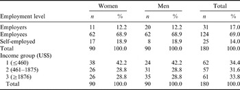
When grouped by employment level, sample distribution showed that most (69%) of the individuals were the offspring of employees; this is consistent with the results found in recent economic and social surveys carried out in Merida, Yucatan. For example, according to the National Survey of Occupation and Employment 2009, the employment level percentages are: employers, 5%; employees, 74.8%; and self-employed, 16.7% (INEGI, 2010). The distribution was more balanced in the number of subjects by income group, as is to be expected when grouping by terciles. These trends were present overall and by sex (Table 1).
Sample sex distribution by employment level and income group

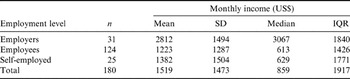
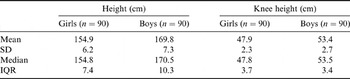
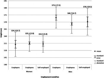
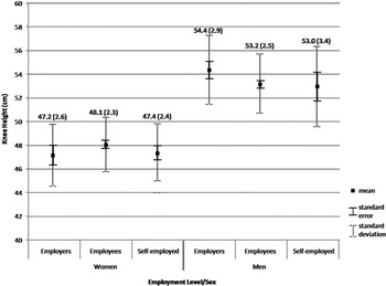
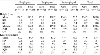
Differences (p<0.001, Kruskal–Wallis) were observed in total family income by employment level between employers (3067 US$) and employees (613 US$) and employers (3067 US$) and the self-employed (629 US$) (Table 2). Means for height (t 178=−14.83, p<0.001) and knee height (t 178=−14.66, p<0.001) were higher for boys than for girls (Table 3). No differences were present by age so the two age groups were pooled into a single group by sex. The daughters of employees had higher mean height and knee height values than the daughters of employers and the self-employed (Figs 1 and 2). However, these differences were not statistically significant. For men, the sons of employers had the highest mean height and knee height values, but these were not significantly higher than those of the sons of employees and the self-employed.
Descriptive statistics of monthly income (in US$) by employment level
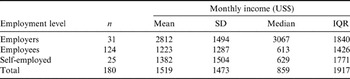
IQR, interquartile range.
Kruskal–Wallis: χ 22=27.6, p<0.001.
Height and knee height descriptive statistics by sex
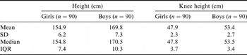
SD, standard deviation; IQR, interquartile range.
Mean height (SD) by employment level and sex.

Mean knee height (SD) by employment level and sex.

The greatest variation in the studied variables, expressed as standard deviations, was observed in the daughters of employers and the sons of the self-employed. However, both variables exhibited very low coefficients of variation and, contrary to expectation, there was a high level of similarity among the three employment levels; in other words, variation was homogeneous within each studied group (Table 4).
Height and knee height descriptive statistics by sex and employment level
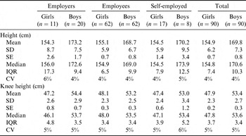
SD, standard deviation; SE, standard error; IQR, interquartile range; CV, coefficient of variation.
Height by employment level: girls F=0.11 (p=0.896), boys F=3.06 (p=0.051); knee height by employment level: girls F=1.33 (p=0.271), boys F=1.77 (p=0.175).
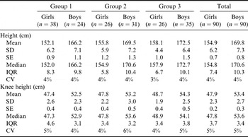
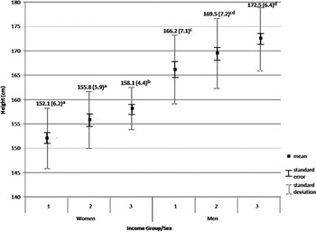
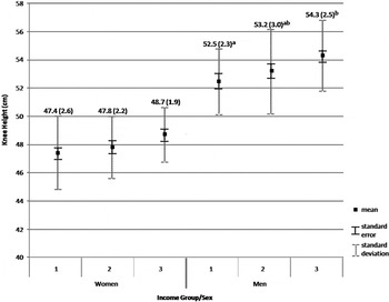
In contrast to the employment level analyses, mean height and knee height in boys and girls increased as family income increased (Table 5, Figs 3 and 4). No clear pattern, like in the means, was distinguished in the standard deviations of growth measurements, except for girls, whose standard deviations decreased as family income increased. Between income groups, the coefficients of variation were low and similar, while variations were homogeneous within these groups.
Height and knee height descriptive statistics by income group (US$) and sex
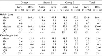
Group 1: ≤460 US$; Group 2: 461–1875 US$; Group 3: ≥1876 US$.
SD, standard deviation; SE, standard error; IQR, interquartile range; CV, coefficient of variation.
Height by income group: girls F=8.92 (p<0.001), boys F=5.92 (p=0.004); knee height by income group: girls F=2.19 (p=0.118), boys F=3.36 (p=0.039).
Mean height (SD) by income group and sex. Women: significant differences (p<0.05) between a and b Bonferroni multiple comparisons. Men: significant differences (p<0.05) between c and d; Group 2 had no significant differences with other groups; Bonferroni multiple comparisons.

Mean knee height (SD) by income group and sex. Men: significant differences (p<0.05) between a and b Bonferroni multiple comparisons.

Discussion
A significant trend (p<0.05, one-way ANOVA) was found in the absolute measurements of height and knee height for income group: as family income increased both girls and boys were taller and had higher knee height, but no such trend was visible between employment level categories (Table 5, Figs 3 and 4). Employment level categories were organized under the assumption that employers could offer their offspring a more favourable growth environment, followed by salaried employees and the self-employed. The results did not support this assumption for boys or girls, or for the two analysed somatic variables. This was the case even though average income for employers was considerably higher than for the other employment level categories. However, it was recognized that the size of some of the employment groups was very small, which limits the scope of the statistical analysis.
Differences were present between income Groups 3 and 1 in height (p=0.003) and knee height (p=0.04) for boys, which coincides with previous reports (Frisancho et al., Reference Frisancho, Gilding and Tanner2001; Malina et al., Reference Malina, Peña Reyes and Little2009). For girls, differences were observed in height between Groups 1 and 3 (p<0.001) and Groups 2 and 3 (p=0.038).
Use of total family income as a classification criterion produced clear differences between groups with higher significance levels than the results by employment level. This discrepancy could be attributed to the fact that income has a greater effect than employment level on family lifestyle in terms of quality of housing and medical care, access to services and food security. In general adolescents in Group 3 have significantly more access to piped water inside the house (χ 2(2)=15.14, p<0.001), and to toilet with sink (Fisher's exact=15.33, p<0.001), access to better health care services (χ 2(4)=55.54, p<0.001) and less overcrowding (χ 2(2)=37.56, p<0.001). Also, the education level of their parents is higher than in the other income groups (r s=0.739; r s=0.709, for fathers and mothers; p<0.001 in both cases).
Variance was highest in the boys of the self-employed, which agrees with Harrison and Schmitt's proposal (Table 4, Figs 1 and 2). No differences were observed, however, in height and knee height variance by income group or employment level, and the coefficients of variation were very low and similar in both cases (Tables 4 and 5). This indicates that relative variation within each subgroup was homogeneous.
In contrast to Bogin's findings, differences were found in the means and variations between income groups because income within these groups is highly variable (group means: 1=337, 2=920 and 3=3067 US$; inter-tercile range: 1=169, 2=613 and 3=1533 US$). However, the overall results are comparable to those of Bogin (Reference Bogin1991) already reported in the Introduction. In his study, height was most variable in the low socieconomic group and least variable in the high socieconomic group. Nevertheless, Bogin compared the means of the coefficients of variation because he had at least four coefficients of variation per sample, each corresponding to annual intervals. Because we had a single measurement, there was only one coefficient of variation per income group and employment level.
It is possible that the differences in height observed here can be attributed to the fact that the employer group consists of businessmen who own their own companies, and who had significantly higher (p<0.001, Kruskal–Wallis) income than the other employment levels and, consequently, greater access to better health care services (χ 2(4)=24.16, p<0.001). In addition, the employers and their wives had significantly higher formal education levels than those in the other employment levels (χ 2(4)=10.19; χ 2(4)=16.71, for fathers and mothers; p<0.05 in both cases). The employee and self-employed groups were heterogeneous in terms of income since some heads of household in these groups earned income similar to the employers, while others had monthly incomes lower than 613 US$ (Table 2).
The results differ from previous reports in terms of the magnitude of differences in growth by social group (Nystrôm-Peck & Vagero, Reference Nystrôm-Peck and Vagero1987; Silventoinen et al., Reference Silventoinen, Lahelma and Rahkonen1999; Komlos & Kriwy, Reference Komlos and Kriwy2003; Heineck, Reference Heineck2006). Using subjects' parental education level and occupation, Nystrôm-Peck & Vagero (Reference Nystrôm-Peck and Vagero1987) reported height differences of 3.9 cm in men and 1.4 cm in women. For men, this difference is smaller than the 4.5 cm observed here between the employer and employee levels, while the difference for women was higher than the <1 cm recorded here between each employment level. These discrepancies are probably due to Sweden having less marked social inequality than Mexico, resulting in less differentiated health conditions and growth.
To test the hypothesis that environmental effects are more clearly manifested in body proportionality, Frisancho et al. (Reference Frisancho, Gilding and Tanner2001) analysed the relationship between leg length and seated height and income poverty index for a group of 2985 Mexican–Americans aged 2–17 years using data collected from 1988 to 1994 as part of the third United States National Health and Nutrition Survey (NHANES III). The data indicated that differences in relative leg length associated with differences (p<0.01) in the income poverty proportion were not reflected in differences in sitting height; the authors concluded that the influence of environmental factors such as socioeconomic status is greater for leg length than seated height.
In this same sense, Silventoinen et al. (Reference Silventoinen, Lahelma and Rahkonen1999) analysed monetary income as a life condition associated with physical growth. In Silventoinen's study, subjects who had experienced economic difficulties during childhood were 0.59 cm (men) and 0.48 cm (women) shorter than those who had not; these differences are much smaller than observed here. The smaller differences reported by Silventoinen et al. (Reference Silventoinen, Lahelma and Rahkonen1999) are probably a result of the subjects being from the same geographic zone and the same urbanization level, meaning the group was more homogeneous in terms of social and economic conditions. The absence of large differences in somatic variables can also be explained by a lack of sufficiently large economic differences between social groups in Finland, and the fact that 73% of their sample of both sexes stated that they had not experienced economic difficulties during childhood.
Conclusions
In the adolescent girls in this study, the highest income tercile (Group 3) had the least variation in height and knee height. No clear pattern was observed in differences in height and knee height by employment level, either in mean values or variability. This means that the original study hypothesis was rejected for this classification. The hypothesis applies partially to the income group classification since clear increases in height and knee height were linked to higher income, but not to variation. Height and knee height coefficients of variation for employment and income categories were low and similar, suggesting that each category was relatively homogeneous. In the present sample, similarities among lower income and lower employment level families did not result in higher variation in the studied growth measurements. Differences in growth between income groups differ from those between employment level groups because income has a greater effect on a family's quality and style of life: housing, access to services, quality of medical care and food security.
Acknowledgments
The research reported here forms part of the project Ecología Humana de la Migración en Yucatán financed by the Consejo Nacional de Ciencia y Tecnología de México (Conacyt 59994-H) from which AV received a scholarship for writing her undergraduate thesis at the Faculty of Medicine, Universidad Autónoma de Yucatán. The authors thank Ana C. Andrade, Enna Basulto, Rocío Higuera, Patricia Quiróz and Mario Rivero for assistance with the field work, as well as Armando Rojas and Graciela Valentín for standardizing anthropometric equipment, field data collection and logistical support. The final version of this paper was written at the University of Loughborough, United Kingdom, where one of the authors (FD) spent a sabbatical year thanks to a fellowship from Conacyt (No. 166138).