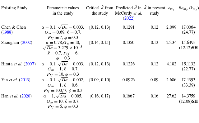
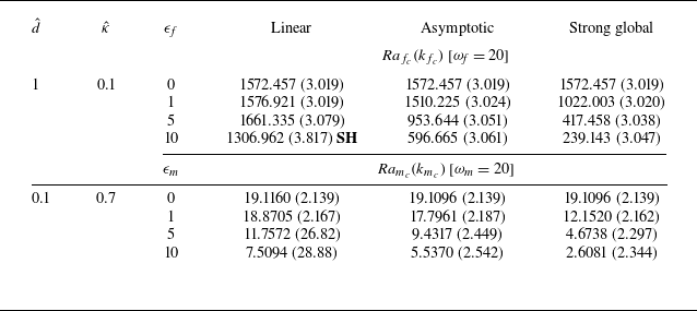
1. Introduction
Investigations concerning natural convective instability occurring in various geophysical and environmental processes have been performed by numerous researchers in order to identify and regulate the criteria under which instability arises within a system. The studies involving the paradigmatic situation of Rayleigh–Bénard instability and its porous medium counterpart, also known as Darcy–Bénard instability, are well documented in the monographs by Bhattacharjee (Reference Bhattacharjee1987), Getling (Reference Getling1998), Nield & Bejan (Reference Nield and Bejan2006) and Chandrasekhar (Reference Chandrasekhar2013), Joseph (Reference Joseph2013). Understanding the dynamics of these thermoconvective systems contributes to our comprehension of physical phenomena and holds significant relevance for practical applications in geophysics, environmental science and energy resource exploration. The monographs by Ingham & Pop (Reference Ingham and Pop2002) and Bejan (Reference Bejan2013) mention several case studies wherein understanding these phenomena has been vital. There are several thermoconvective phenomena in which a porous medium is encountered lying under a fluid layer in many geophysical and industrial set-ups (Prasad Reference Prasad1991), which has motivated numerous researchers in the past few decades to study the heat and mass transfer phenomenon in a superposed fluid–porous-layer (SFPL) system. Geophysical areas where convection in the SFPL system can be observed are the retrieval of oil from underground reservoirs (Allen, Behie & Trangenstein Reference Allen, Behie and Trangenstein2013), the flow of contaminants in groundwater reservoirs (Habel, Mendoza & Bagtzoglou Reference Habel, Mendoza and Bagtzoglou2002), the flow of water underneath the surface of the earth (Cardenas Reference Cardenas2015) and the mushy layer of ice crystals below sea ice (Wells, Hitchen & Parkinson Reference Wells, Hitchen and Parkinson2019). Industrial applications that feature convection in an SFPL system are the solidification of concentrated alloys (Le Bars & Worster Reference Le Bars and Worster2006), the construction of composite materials for automobile industries (Blest et al. Reference Blest, Duffy, McKee and Zulkifle1999a ,Reference Blest, McKee, Zulkifle and Marshall b ) and the cooling of electronic components in electronic devices (Al-Zamily Reference Al-Zamily2017). Understanding heat transfer in such superposed systems can help examine many geothermal sources and engineering environments (McCurdy, Moore & Wang Reference McCurdy, Moore and Wang2022).
Sun (Reference Sun1973) was the first to study the commencement of thermal convection in an SFPL system. Nield (Reference Nield1977) extended this work (Sun Reference Sun1973) by considering the effect of surface tension at the upper boundary of the fluid domain. He considered the upper surface to be deformable and obtained a closed-form solution for constant heat-flux boundary conditions. Chen & Chen (Reference Chen and Chen1988) studied the porous–fluid-layer problem with the effect of a salinity gradient. The authors observed the influence of the depth ratio on the onset of convective instability in the natural convection case and discovered the change in instability mode from porous mode to fluid mode for a depth ratio
 ${\gt } 0.1$
, which was overlooked by Sun (Reference Sun1973). Later, the authors verified their published theoretical results through an experimental study (Chen & Chen Reference Chen and Chen1989). Taslim & Narusawa (Reference Taslim and Narusawa1989) performed a linear instability analysis by considering three different structural arrangements of the convective instability in the multi-layer systems. They studied the effects of the thermal diffusivity ratio, the Darcy number and the Beavers–Joseph coefficient in an SFPL system with layers of the same depth. Further, Straughan (Reference Straughan2001, Reference Straughan2002) investigated the two-layer problem with and without the surface tension effect at the upper surface of the fluid domain. Straughan (Reference Straughan2001) confirmed the bi-modal nature of the convective flow in an SFPL system, as observed earlier by Chen & Chen (Reference Chen and Chen1988). Later, Straughan (Reference Straughan2002) remarked that the convection being dominant in the fluid or the porous layer could be altered by varying system parameters such as depth ratio, diffusivity ratio and Beavers–Joseph constant. Prasad (Reference Prasad1991) reviewed the findings regarding thermal convection in SFPL systems and reported that the interaction between fluid and porous domains is prevalent even in the case of a densely packed porous medium. Bagchi & Kulacki (Reference Bagchi and Kulacki2014) documented theoretical and experimental results concerning natural convection in superposed systems.
The nonlinear stability analysis for SFPL systems has been assessed only to a limited extent because the nonlinear advection term produces a sign indefinite term in the equation for the evolution of energy functional. Payne & Straughan (Reference Payne and Straughan1998) and Hill & Straughan (Reference Hill and Straughan2009) were the first to construct the nonlinear energy stability bounds for an SFPL system. The Stokes equation instead of the Navier–Stokes equation was employed to model the flow in the fluid domain, and the hindrance due to the advection term can be avoided. Moreover, a highly porous material underlying a fluid layer was considered so that the Brinkman law can govern the fluid flow through it. Thus, the convective term in the governing equation for the porous domain manages the term in the equation for the fluid domain. Hill & Carr (Reference Hill and Carr2010) employed a viscoelastic model to develop the nonlinear stability limits. Later, McCurdy, Moore & Wang (Reference McCurdy, Moore and Wang2019) argued that the use of Stokes equations, and restricting porosity to be large when using the Brinkman law, may be conservative, and the nonlinear stability thresholds for Navier–Stokes–Darcy flow are still left for inspection. The authors proposed to employ the Lions interface condition (see Discacciati & Quarteroni Reference Discacciati and Quarteroni2009, and references therein), incorporating a dynamic pressure term in the normal force balance equation at the interface. The authors also recommended that one more requirement for the development of an energy law was to impose the Beavers–Joseph–Saffman–Jones (BJSJ) condition (see Discacciati & Quarteroni Reference Discacciati and Quarteroni2009) instead of the Beavers–Joseph condition, balancing the tangential stress at the interface. In all these studies, the bounds produced by linear and nonlinear analyses are found to be in agreement, and a very small region of subcritical instability is possible.
Recently, using the centre manifold reduction theory, Han, Wang & Wang (Reference Han, Wang and Wang2020) examined the dynamic transitions of convective instability from one flow regime to another and found jump transitions can happen for specific values of parameters in an SFPL system. Anjali, Khan & Bera (Reference Anjali, Khan and Bera2022) investigated the effect of anisotropy and inhomogeneity of the porous medium on the thermal convection in the SFPL system enforced with plane Poiseuille flow. The authors brought information about the reason behind bimodal instability by carrying out an energy budget analysis. More studies on the convective instability in SFPL systems with different configurations are reported in the literature (see Kolchanova & Kolchanov Reference Kolchanova and Kolchanov2021, McCurdy et al. Reference McCurdy, Moore and Wang2022 and references therein).
Notably, the mechanisms to control the instability in thermoconvective processes are essential in understanding the intricate dynamics to prevent unwanted consequences and to allow us to optimise the process outcome. Control on the onset of instability can be achieved by utilising external factors added to the convection configuration, such as involving parameters depending on time (temperature and gravity), rotating the system and imposing a magnetic field. The study of the effect of modulation on the commencement of thermal convection originated when Donnelly (Reference Donnelly1964) experimentally investigated the stability of the flow between rotating cylinders with a periodic angular speed. Venezian (Reference Venezian1969) was the first to study the thermal analogue of Donnelly’s experiments by considering the classical Rayleigh–Bénard convection (RBC) problem with modulated boundary temperatures. Later, Rosenblat & Tanaka (Reference Rosenblat and Tanaka1971) and Yih & Li (Reference Yih and Li1972) discussed the influence of the modulated temperature field on RBC with different boundary combinations. These studies aimed to find whether the onset of instability in the classical RBC problem can be regulated by introducing a temperature field that varies sinusoidally with time. The instability may set in synchronously or sub-harmonically in response to the external vibrations (Yih & Li Reference Yih and Li1972). Recently, many researchers have investigated the linear instability thresholds of thermally modulated convection in a fluid layer with different configurations (see Hazra, Kumar & Mitra Reference Hazra, Kumar and Mitra2020, Christopher, Le Bars & Smith Reference Christopher, Le Bars and Smith2023 and references therein). The nonlinear stability analysis of a modulated RBC was first considered by Homsy (Reference Homsy1974). The possibility of the subcritical region due to modulation was observed. The strong stability thresholds were found to be smaller than both linear and asymptotic thresholds. Following the pioneering work of Homsy (Reference Homsy1974), many researchers investigated the nonlinear stability bounds for time-dependent flows under different hydrodynamic arrangements, which are well documented in the article of Dev, Suthar & Siddheshwar (Reference Dev, Suthar and Siddheshwar2024) and references therein.
The porous media analogue of the problem of the influence of a modulated temperature in a fluid layer was first examined by Caltagirone (Reference Caltagirone1976). Chhuon & Caltagirone (Reference Chhuon and Caltagirone1979) explored the effect of a periodic thermal distribution on thermal convection in a porous layer by employing the Darcy model for the governing equations. They applied the Floquet theory to acquire the critical parameters determining convective instability and observed that the time-periodic temperature distribution exhibited a destabilising effect. Rudraiah & Malashetty (Reference Rudraiah and Malashetty1990) considered natural convection in a porous medium of high porosity and time-dependent thermal boundaries using the Brinkman model. Several authors performed linear instability analyses of the modulation problem in a porous medium with different convective configurations (Bhadauria Reference Bhadauria2008; Bansal & Suthar Reference Bansal and Suthar2022). Recently, Saravanan & Meenasaranya (Reference Saravanan and Meenasaranya2017) conducted a nonlinear stability analysis for a Brinkman layer utilising the energy method and obtained only strong global bounds. Dev et al. (Reference Dev, Suthar and Siddheshwar2024) investigated modulated Brinkman–Bénard convection in a porous box and obtained strong and asymptotic bounds.
It can be observed from the literature available on the convective instability in an SFPL system (Bagchi & Kulacki Reference Bagchi and Kulacki2014) that the effect of the various fluid and porous material properties, the thickness of the layers in the SFPL system and different conditions at the porous–fluid interface on the commencement of thermal convection in an SFPL system have been studied. However, the influence of a time-dependent boundary temperature of a superposed system comprising a fluid and porous medium still needs to be explored despite its utility as a control mechanism as well as its obvious occurrence in numerous real-world scenarios like in solar ponds primarily due to the diurnal cycle of solar radiation. We remark here that a typical solar pond may be divided into three zones, viz. upper, lower and non-convective zones when a salinity gradient is present. Some recent studies introduced a porous bed in the lower convective zone of a typical solar pond, i.e. at the bottom of the solar pond, and found that the inclusion of a porous bed stabilises the system (Hill & Carr Reference Hill and Carr2013a , Reference Hill and Carrb ). A restrictive study may consider a saltless solar pond (Hull Reference Hull1980); accordingly, a physical comparison will need the absence of salinity. Even with this simplification, the physics of the problem is intriguing and raises several questions regarding the effect of modulation on convective instabilities in the two-layer system. The main queries are: Can a periodic thermal distribution’s effect on the instability alter its course? Can applying modulation enable the system to control the dynamic transition of the instability mode in an SFPL system without changing its properties? Does nonlinear analysis lead to the possibility of a subcritical instability region? Are subcritical instabilities possible in the presence of modulation?
The present study aims to find the answers to these questions by investigating four different configurations of SFPL systems with a time-periodic temperature applied at the lower wall of the medium with fixed porous structure. The heat transfer from the upper surface is controlled by considering a mixed thermal boundary condition depending on the Biot number. The present article consists of five sections: the outline of the problem set-up and corresponding governing equations are given in § 2. The numerical method and stability analyses are articulated in § 3. The results and comparison of linear and nonlinear thresholds are presented in § 4. The conclusions drawn from the present study are documented in § 5.
2. Mathematical formulation
Consider a system consisting of a horizontal fluid layer superposed on a horizontal porous layer of thicknesses
 $d_{\!f}$
and
 $d_m$
, respectively. We assume a Cartesian coordinate system
 $(x,y,z)$
with the
 $z$
-axis aligned vertically such that the interface of the SFPL lies at the plane
 $z = 0$
, the impermeable lower surface is at the plane
 $z=-d_m$
and the rigid upper surface lies at the plane
 $z = d_{\!f}$
, as depicted in figure 1. The parameter
 $T_0$
denotes the temperature at the interface. A constant temperature
 $T_U$
is maintained at the upper wall of the fluid domain in the basic state. The porous layer is heated from below with a sinusoidally varying temperature
 $T_m$
having a modulation frequency
 $\omega _0$
, a modulation amplitude
 $\epsilon _0$
and a non-zero mean value
 $T_L (T_L \gt T_U)$
. We define
 \begin{equation} T_m = T_L + \epsilon _0 \Delta T \cos (\omega _0t), \quad z= -d_m, \end{equation}
where
 $\Delta T = T_L - T_U$
is the difference between the mean values of bottom and upper boundary temperatures. Two different formulations to model the flow through the permeable interface in the superposed system are debated in the literature: one- and two-domain approaches (Hirata et al. Reference Hirata, Goyeau, Gobin, Carr and Cotta2007, Reference Hirata, Goyeau, Gobin, Chandesris and Jamet2009). Hirata et al. (Reference Hirata, Goyeau, Gobin, Chandesris and Jamet2009) showed the equivalence between the two approaches. Since the two-domain approach offers experimental validation for the published theoretical results (Chen & Chen Reference Chen and Chen1989), we adopt the two-domain approach. The equations expressing the motion of incompressible Boussinesq fluid in the fluid layer are given by
 \begin{align} \boldsymbol{\nabla } \boldsymbol{\cdot } \boldsymbol{u}_{\!f} &=0, \end{align}
 \begin{align} \rho _0 \left (\frac{\partial \boldsymbol{u}_{\!f}}{\partial t} + \boldsymbol{u}_{\!f}\boldsymbol{\cdot } \boldsymbol{\nabla } \boldsymbol{u}_{\!f}\right ) = \boldsymbol{\nabla } \boldsymbol{\cdot } & \left (2\mu \unicode{x1D63F}(\boldsymbol{u}_{\!f}) - p_{\!f} \unicode{x1D644} \kern1.5pt \right ) + \rho _0 [1 - \beta (T_{\!f}-T_0)] \boldsymbol{g}, \end{align}
 \begin{align} \frac{\partial T_{\!f}}{\partial t}+ \boldsymbol{u}_{\!f}\boldsymbol{\cdot }\boldsymbol{\nabla } T_{\!f} &= \frac{\kappa _{\!f}}{(\rho _0 C_p)_{\!f}}{\nabla} ^2 T_{\!f}. \end{align}
Schematic diagram of the SFPL system.

In the above equations,
 $\boldsymbol{u}_{\!f} = (u_{\!f},v_{\!f},w_{\!f}), p_{\!f}, \mu , T_{\!f}, \kappa _{\!f}, C_p, \rho _0$
and
 $\beta$
represent the fluid velocity, pressure, viscosity, temperature, thermal conductivity, specific heat, density at
 $T_{\!f} = T_0$
and coefficient of thermal expansion in the fluid domain, respectively. The rate of strain tensor
 $\unicode{x1D63F}$
is defined as
 $\unicode{x1D63F} = (\boldsymbol{\nabla } \boldsymbol{u}_{\!f} + \boldsymbol{\nabla } \boldsymbol{u}_{\!f}^\top )/{2}$
and
 $\unicode{x1D644}$
is the second-order identity tensor. The vector
 $\boldsymbol{g} = (0,0,-g)$
denotes the acceleration due to gravity, acting in the
 $-\boldsymbol{k}$
direction. In a densely packed porous medium, the fluid flow obeys the Darcy law (Nield & Bejan Reference Nield and Bejan2006; Anjali et al. Reference Anjali, Khan and Bera2022). An alternate way to model the flow in the porous domain is the Brinkman law, which is recommended when the porous medium is sparsely packed (Hill & Straughan Reference Hill and Straughan2009). The limitations of the Brinkman equation in modelling the flow at a porous–fluid interface are discussed by Nield (Reference Nield2009). Furthermore, the porous layer of SFPL systems featured in many geophysical flows has very low porosity (McCurdy et al. Reference McCurdy, Moore and Wang2019). Consequently, we employ Darcy’s law to model the fluid flow through the porous layer. The equations governing the fluid motion in the porous layer are given by
 \begin{align} \boldsymbol{\nabla } \boldsymbol{\cdot } \boldsymbol{u}_m &=0, \end{align}
 \begin{align} \frac{\rho _0}{\phi } \frac{\partial \boldsymbol{u}_m}{\partial t}= -\boldsymbol{\nabla } p_m - \frac{\mu }{K} \boldsymbol{u}_m &+ \rho _0 [1-\beta (T_m-T_0)] \boldsymbol{g}, \end{align}
 \begin{align} \frac{(\rho _0 C_p)_{\textit{eff}}}{(\rho _0 C_p)_{\!f}} \frac{\partial T_m}{\partial t} + \boldsymbol{u}_m\boldsymbol{\cdot }\boldsymbol{\nabla } T_m & = \frac{\kappa _{\textit{eff}}}{(\rho _0 C_p)_{\!f}} {\nabla} ^2 T_m. \\[9pt] \nonumber \end{align}
In the above equations, the variables
 $\boldsymbol{u}_m=(u_m,v_m,w_m)$
and
 $p_m$
denote the fluid velocity and pressure at a point in the porous domain, respectively. The quantities
 $\phi$
and
 $K$
represent the porosity and permeability of the porous medium. The effective thermal conductivity
 $\kappa _{\textit{eff}}$
and the effective volumetric heat capacity
 $(\rho _0 C_p)_{\textit{eff}}$
of the porous medium can be calculated using the relation
 $ X_{\textit{eff}} = \phi X_{\!f} + (1-\phi )X_m$
, by substituting
 $X=\kappa$
and
 $\rho _0C_p.$
The SFPL system is assumed to be confined between a rigid upper boundary and an impermeable lower boundary
 \begin{align} \boldsymbol{u}_{\!f} \boldsymbol{\cdot } \boldsymbol{n} = \boldsymbol{\tau }_i \boldsymbol{\cdot } \boldsymbol{u}_{\!f} & = 0, \quad z = d_{\!f}, \end{align}
 \begin{align} \boldsymbol{u}_m \boldsymbol{\cdot } \boldsymbol{n} & = 0, \quad z = -d_m, \end{align}
where
 $\boldsymbol{n}$
is the unit normal vector in the
 $-z$
direction and
 $\boldsymbol{\tau }_i$
, for
 $i = \{1,2\}$
, are unit tangent vectors. A permeable wall differentiates the fluid and porous domains, and the porous layer is saturated with the overlying fluid. The continuity of normal velocity, temperature and heat flux at the interface
 $\varGamma _{\!f} \,(\text{i.e. the plane}\, z = 0)$
yield
 \begin{align} \boldsymbol{u}_{\!f} \boldsymbol{\cdot } \boldsymbol{n} &= \boldsymbol{u}_m \boldsymbol{\cdot } \boldsymbol{n}, \end{align}
 \begin{align} T_{\!f} = T_m, \quad & \kappa _{\!f} \boldsymbol{\nabla } T_{\!f} \boldsymbol{\cdot } \boldsymbol{n} = \kappa _m \boldsymbol{\nabla } T_m \boldsymbol{\cdot } \boldsymbol{n}. \end{align}
The BJSJ condition is employed to balance the tangential stress at interface
 $\varGamma _{\!f}$
, which is important in the nonlinear energy analysis (Discacciati & Quarteroni Reference Discacciati and Quarteroni2009)
 \begin{equation} - 2 \mu (\unicode{x1D63F} (\boldsymbol{u}_{\!f})\boldsymbol{n}) \boldsymbol{\cdot } \boldsymbol{\tau }_i = \frac{\alpha \mu }{\sqrt {K}} \boldsymbol{u}_{\!f} \boldsymbol{\cdot } \boldsymbol{\tau }_i, \end{equation}
where
 $\alpha$
is the Beavers–Joseph (BJ) constant. In the literature (Prasad Reference Prasad1991; Straughan Reference Straughan2002), two well-known conditions, namely the BJ and Beavers–Joseph–Jones (BJJ) conditions were utilised for linear instability analyses. McCurdy et al. (Reference McCurdy, Moore and Wang2019) showed that all these three conditions yield similar linear instability thresholds in a small Darcy number regime. The condition concerning the balances of normal force at interface
 $\varGamma _{\!f}$
, the Lions interface condition (Discacciati & Quarteroni Reference Discacciati and Quarteroni2009) is given by
 \begin{equation} \left ((-2\mu \unicode{x1D63F}(\boldsymbol{u}_{\!f}) + p_{\!f} \unicode{x1D644}\,)\boldsymbol{n}\right ) \boldsymbol{\cdot } \boldsymbol{n} + \frac{\rho _0}{2} (\boldsymbol{u}_{\!f} \boldsymbol{\cdot } \boldsymbol{u}_{\!f}) = p_m. \end{equation}
2.1. Non-dimensionalisation
It is known that two different scalings (Chen & Chen Reference Chen and Chen1988) for the fluid- and porous-layer variables should be used to recognise the symmetry that the equations in both domains exhibit. We use the following scalings:
 \begin{align} \boldsymbol{r}^\ast _{\!f} &=\frac{1}{d_{\!f}} \boldsymbol{r}, \quad t^\ast _{\!f} = t \frac{\chi _{\!f}}{d_{\!f}^2}, \quad \boldsymbol{u}^\ast _{\!f} = \boldsymbol{u}_{\!f}\frac{d_{\!f}}{\nu }, \quad T^\ast _{\!f} = T_{\!f} \frac{\chi _{\!f}}{(\bar {T}_0 - T_U)\nu }, \quad p^\ast _{\!f} = p_{\!f} \frac{d_{\!f}^2}{\rho _0 \nu ^2}, \end{align}
 \begin{align} \boldsymbol{r}^\ast _m &=\frac{1}{d_m} \boldsymbol{r}, \quad t^\ast _m = t \frac{\chi _m}{d_m^2}, \quad {\boldsymbol{u}}^\ast _m = \boldsymbol{u}_m \frac{d_m}{\nu }, \quad T^\ast _m = T_m \frac{\chi _m}{(T_L - \bar {T}_0)\nu }, \quad p^\ast _m = p_m \frac{d_m^2}{\rho _0 \nu ^2}, \end{align}
where
 $\boldsymbol{r} = (x,y,z)$
, the superscript asterisk
 $(^\ast )$
represents the non-dimensional variables and the quantities
 $\chi _{\!f} ={\kappa _{\!f}}/{(\rho _0 C_p)_{\!f}}$
and
 $\chi _m = {\kappa _{\textit{eff}}}/{(\rho _0 C_p)_{\!f}}$
are thermal diffusivities for the fluid and porous domains, respectively,
 $\nu$
is the kinematic viscosity and
 $\bar {T}_0$
represents the steady part of the interface temperature and is given in Appendix A. Since the dimensional times for the fluid and porous domains must be the same, the relation between the non-dimensional time variables is obtained (after dropping the asterisks) as
 $ t_m = ({{\hat {d}}^2}/{\hat {\kappa }}) t_{\!f}$
, where
 $\hat {d}={d_{\!f}}/{d_m}$
is defined as the ratio of the depth of the fluid domain to the depth of the porous domain, and
 $\hat {\kappa } = {\chi _{\!f}}/{\chi _m} = {\kappa _{\!f}}/{\kappa _{\textit{eff}}}$
is defined as the ratio of fluid to porous heat diffusivities. The above scaling is introduced in the system (2.2)–(2.7), and we obtain the non-dimensional governing equations for fluid and porous domains (sans asterisks) as
 \begin{align} \boldsymbol{\nabla }_{\!f} \boldsymbol{\cdot } \boldsymbol{u}_{\!f} &= 0, \end{align}
 \begin{align} \frac{1}{{\textit{Pr}}_{\!f}} \frac{\partial \boldsymbol{u}_{\!f}}{\partial t_{\!f}} + (\boldsymbol{u}_{\!f}\boldsymbol{\cdot } \boldsymbol{\nabla }_{\!f}) \boldsymbol{u}_{\!f} = 2 \boldsymbol{\nabla }_{\!f} \boldsymbol{\cdot } \unicode{x1D63F} (\boldsymbol{u}_{\!f}) & - \boldsymbol{\nabla }_{\!f} p_{\!f} + Ra_{\!f} T_{\!f} \boldsymbol{k} + \frac{d^3_{\!f}}{\nu ^2} (1+\beta T_0)\boldsymbol{g}, \end{align}
 \begin{align} \frac{\partial T_{\!f}}{\partial t_{\!f}} + \textit{Pr}_{\!f}(\boldsymbol{u}_{\!f}\boldsymbol{\cdot } \boldsymbol{\nabla }_{\!f}) T_{\!f} &= \boldsymbol{\nabla} _{\!f}^2 T_{\!f}, \end{align}
 \begin{align} \boldsymbol{\nabla }_m \boldsymbol{\cdot } \boldsymbol{u}_m &= 0, \end{align}
 \begin{align} \frac{Da}{\phi \textit{Pr}_m} \frac{\partial \boldsymbol{u}_m}{\partial t_m} = -Da \boldsymbol{\nabla }_m p_m -\boldsymbol{u}_m &+ Ra_m T_m \boldsymbol{k} + \frac{Kd_m}{\nu ^2} (1+\beta T_0)\boldsymbol{g}, \end{align}
 \begin{align} G_m \frac{\partial T_m}{\partial t_m} + \textit{Pr}_m (\boldsymbol{u}_m\boldsymbol{\cdot } \boldsymbol{\nabla }_m) T_m &= \boldsymbol{\nabla} _m^2 T_m, \end{align}
where the non-dimensional physical parameters
 $Da = {K}/{d_m^2}, \textit{Pr}_{\!f} ={\nu }/{\chi _{\!f}}$
and
 $ \textit{Pr}_m = {\nu }/{\chi _m},$
are the Darcy number, and the Prandtl numbers for the fluid and porous domains, respectively. The parameter
 $G_m = {(\rho _0 C_p)_{\textit{eff}}}/{(\rho _0 C_p)_{\!f}}$
represents the ratio of porous to fluid volumetric heat capacities and
 $Ra_{\!f}$
and
 $Ra_m$
are the Rayleigh numbers for the fluid and porous domains, respectively, and are defined as
 \begin{equation} Ra_{\!f} = \frac{\beta \rho _0 g (\bar {T}_0-T_U) d_{\!f}^3}{\mu \chi _{\!f}}, \quad Ra_m = \frac{\beta \rho _0 g (T_L-\bar {T}_0) K d_m }{\mu \chi _m}. \end{equation}
The relation
 $ Ra_m =({Da \hat {\kappa }^2}/{\hat {d}^4}) Ra_{\!f}$
can be readily observed from the definition. The wall temperatures in the non-dimensional form are given by
 \begin{eqnarray} T_{\!f} &\!\!=\!\!& \frac{1}{{\textit{Pr}}_{\!f}}\frac{T_U}{(\bar {T}_0 - T_U)}, \quad \quad \quad \quad \quad \quad \quad \quad \quad \quad z_{\!f} = 1, \nonumber\\ T_m &\!\!=\!\!& \frac{1}{{\textit{Pr}}_m} \left [ \frac{T_L}{(T_L - \bar {T}_0)} + \epsilon _m \cos (\omega _mt_m)\right ]\! , \quad z_m = -1, \end{eqnarray}
where the quantities
 $\epsilon _m = {\epsilon _0 \Delta T}/{(T_L - \bar {T}_0)}$
and
 $\omega _m = {\omega _0 d_m^2}/{\chi _m}$
are the modulation amplitude and the non-dimensional modulation frequency, respectively, in the porous domain. The interfacial conditions in non-dimensional form are given as
 \begin{align} \hat {d} T_{\!f} = \hat {\kappa }^2 T_m, \quad & \boldsymbol{\nabla }_{\!f} T_{\!f} \boldsymbol{\cdot } \boldsymbol{n} = \hat {\kappa } \boldsymbol{\nabla }_m T_m \boldsymbol{\cdot } \boldsymbol{n}, \end{align}
 \begin{align} \boldsymbol{u}_{\!f} \boldsymbol{\cdot } \boldsymbol{n} = \hat {d} \boldsymbol{u}_m \boldsymbol{\cdot } \boldsymbol{n}, \quad & - 2 \left (\unicode{x1D63F} (\boldsymbol{u}_{\!f})\boldsymbol{n}\right ) \boldsymbol{\cdot } \boldsymbol{\tau }_i = \frac{\hat {d} \alpha }{\sqrt {Da}} \boldsymbol{u}_{\!f} \boldsymbol{\cdot } \boldsymbol{\tau }_i, \end{align}
 \begin{align} ((-2\unicode{x1D63F}(\boldsymbol{u}_{\!f}) + p_{\!f} \unicode{x1D644}\,)\boldsymbol{n}) \boldsymbol{\cdot } & \boldsymbol{n} + \frac{1}{2} \vert {\boldsymbol{u}_{\!f}}\vert ^2 = \hat {d}^2 p_m. \end{align}
2.2. Basic state and perturbed system
The fluid is considered at rest in the basic state. We consider the solution in the basic state of the form
 \begin{align} \boldsymbol{u}_{\textit{fb}} &= \boldsymbol{0}, \quad p_{\!f} = p_{\textit{fb}}(z_{\!f},t_{\!f}), \quad T_{\!f} = T_{\textit{fb}}(z_{\!f},t_{\!f}) = \bar {T}_{\!f}(z_{\!f}) + \epsilon _0 \tilde {T}_{\!f}(z_{\!f},t_{\!f}), \end{align}
 \begin{align} \boldsymbol{u}_{mb} &= \boldsymbol{0}, \quad p_m = p_{\textit{mb}}(z_m,t_{\!f}), \quad T_m = T_{\textit{mb}}(z_m,t_m) = \bar {T}_m(z_m) + \epsilon _0\tilde {T}_m(z_m,t_m). \end{align}
Note that the basic state temperatures of the fluid and porous domains have two components each: steady components
 $(\bar {T}_{\!f},\bar {T}_m)$
and oscillatory components
 $(\tilde {T}_{\!f},\tilde {T}_m)$
. To obtain the oscillatory part of the basic state temperatures, we use a general thermal boundary condition at the upper surface,
 $z_{\!f} = 1$
(Straughan Reference Straughan2001; Or & Kelly Reference Or and Kelly2002)
 \begin{equation} \frac{\partial \tilde {T}_{\!f}}{\partial z_{\!f}} = Bi \tilde {T}_{\!f}, \end{equation}
where
 $\textit{Bi}$
is the Biot number. Thus, the basic state temperature is obtained from (2.18)–(2.21), and boundary conditions (2.23), (2.24) and (2.29)
 \begin{align} T_{\textit{fb}} &= \frac{1}{{\textit{Pr}}_{\!f}} \left [ \left ( \frac{\bar {T}_0}{\bar {T}_0-T_U} - z_{\!f} \right ) + \epsilon _{\!f} {\textrm{Re}} \left ( f(z_{\!f})e^{\text{i}\omega _{\!f} t_{\!f}} \right ) \right ]\!, \end{align}
 \begin{align} T_{\textit{mb}} &= \frac{1}{{\textit{Pr}}_m} \left [ \left ( \frac{\bar {T}_0}{T_L-\bar {T}_0} - z_m \right ) + \epsilon _m {\textrm{Re}} \left ( g(z_m)e^{\text{i}\omega _m t_m} \right ) \right ]\!, \end{align}
where
 ${\textrm{Re}}(\boldsymbol{\cdot })$
denotes the real part of its argument. The modulation amplitude
 $\epsilon _{\!f}$
and frequency
 $\omega _{\!f}$
in the fluid layer are given by
 $\epsilon _{\!f} = { \epsilon _0 \Delta T}/(\bar {T}_0-T_U) = ({\hat {\kappa }}/{\hat {d}}) \epsilon _m$
and
 ${\omega _{\!f}} =\omega _0 {d_{\!f}^2}/{\chi _{\!f}} = ({\hat {d}^2}/{\hat {\kappa }})\omega _m$
. The expressions for
 $f(z_{\!f})$
and
 $g(z_m)$
are given in Appendix B. Since the temperature continuity is imposed at the interface
 $\varGamma _{\!f}$
, the fluid- and porous-layer temperatures
 $T_{\!f}$
and
 $T_m$
, respectively, must equal
 $T_0$
, which also consists of steady
 $\bar {T}_0$
and oscillatory
 $\tilde {T}_0$
components, as given in Appendix A.
We introduce the following disturbances to the basic state to analyse the stability of the basic state as:
 \begin{align} \boldsymbol{u}_{\!f} = \boldsymbol{u}^{\prime}_{\!f},\quad p_{\!f} = p_{\textit{fb}} + p^{\prime}_{\!f}, \quad T_{\!f} = T_{\textit{fb}} + \theta _{\!f}, \end{align}
for the fluid-layer variables and
 \begin{align} \boldsymbol{u}_m = \boldsymbol{u}^{\prime}_m , \quad p_m = p_{\textit{mb}} + p^{\prime}_m, \quad T_m = T_{\textit{mb}} + \theta _m, \end{align}
for the porous domain variables. The quantities with the prime
 $(^{\prime})$
represent the perturbed ones. The governing equations for the perturbed quantities are obtained by substituting the above perturbations to the system (2.16)–(2.21) and using the time scale
 $\hat {k}/ \hat {d}^2$
for the porous domain. After dropping the primes, the governing equations for perturbed quantities are
 \begin{align} \boldsymbol{\nabla }_{\!f} \boldsymbol{\cdot } \boldsymbol{u}_{\!f} &= 0, \end{align}
 \begin{align} \frac{1}{{\textit{Pr}}_{\!f}} \frac{\partial \boldsymbol{u}_{\!f}}{\partial t_{\!f}} + (\boldsymbol{u}_{\!f}\boldsymbol{\cdot } \boldsymbol{\nabla }_{\!f}) \boldsymbol{u}_{\!f} & = 2 \boldsymbol{\nabla }_{\!f} \boldsymbol{\cdot } \unicode{x1D63F} (\boldsymbol{u}_{\!f}) - \boldsymbol{\nabla }_{\!f} p_{\!f} + Ra_{\!f} \theta _{\!f} \boldsymbol{k}, \end{align}
 \begin{align} \frac{\partial \theta _{\!f}}{\partial t_{\!f}} + \textit{Pr}_{\!f}(\boldsymbol{u}_{\!f}\boldsymbol{\cdot } \boldsymbol{\nabla }_{\!f}) \theta _{\!f} & = {\nabla} _{\!f}^2 \theta _{\!f} - \textit{Pr}_f w_f \frac{ \partial T_{\textit{fb}}}{\partial z_f}, \end{align}
 \begin{align} \boldsymbol{\nabla }_m \boldsymbol{\cdot } \boldsymbol{u}_m &= 0, \end{align}
 \begin{align} \frac{Da}{\phi \textit{Pr}_m}\frac{\hat {\kappa }}{\hat {d}^2} \frac{\partial \boldsymbol{u}_m}{\partial t_{\!f}} &= -Da \boldsymbol{\nabla }_m p_m -\boldsymbol{u}_m + Ra_m \theta _m \boldsymbol{k}, \end{align}
 \begin{align} G_m \frac{\hat {\kappa }}{\hat {d}^2} \frac{\partial \theta_m }{\partial t_{\!f}} + \textit{Pr}_m (\boldsymbol{u}_m\boldsymbol{\cdot } \boldsymbol{\nabla }_m) \theta _m &= {\nabla} _m^2 \theta _m- \textit{Pr}_m w_m \frac{ \partial T_{\textit{mb}}}{\partial z_m}, \end{align}
subject to boundary conditions
 \begin{align} \boldsymbol{u}_m \boldsymbol{\cdot } \boldsymbol{n} = 0, \quad \theta _m = 0, \quad \text{at} \quad z_m = -1, \\[-28pt] \nonumber \end{align}
 \begin{align} \boldsymbol{u}_{\!f} \boldsymbol{\cdot } \boldsymbol{n} = \boldsymbol{\tau }_i \boldsymbol{\cdot } \frac{\partial \boldsymbol{u}_{\!f} }{\partial \boldsymbol{n}} =- \boldsymbol{\nabla }_{\!f} \theta _{\!f} \boldsymbol{\cdot } \boldsymbol{n} + Bi\theta _{\!f} = 0, \quad \text{at} \quad z_{\!f} = 1, \\[-28pt] \nonumber \end{align}
 \begin{align} \hat {d} \theta_{\!f} = \hat {\kappa }^2 \theta_m, \quad \boldsymbol{\nabla }_{\!f} \theta _{\!f} \boldsymbol{\cdot } \boldsymbol{n} = \hat {\kappa } \boldsymbol{\nabla }_m \theta _m \boldsymbol{\cdot } \boldsymbol{n}, \\[-28pt] \nonumber \end{align}
 \begin{align} \boldsymbol{u}_{\!f} \boldsymbol{\cdot } \boldsymbol{n} = \hat {d} \boldsymbol{u}_m \boldsymbol{\cdot } \boldsymbol{n}, \quad - 2 (\unicode{x1D63F} (\boldsymbol{u}_{\!f})\boldsymbol{n}) \boldsymbol{\cdot } \boldsymbol{\tau }_i = \frac{\hat {d} \alpha }{\sqrt {Da}} \boldsymbol{u}_{\!f} \boldsymbol{\cdot } \boldsymbol{\tau }_i, \\[-28pt] \nonumber \end{align}
 \begin{align} ((-2\unicode{x1D63F}(\boldsymbol{u}_{\!f}) + p_{\!f} \unicode{x1D644}\,)\boldsymbol{n}) \boldsymbol{\cdot } \boldsymbol{n} + \frac{1}{2} |{\boldsymbol{u}_{\!f}}|^2 = \hat {d}^2 p_m, \quad \text{at} \, z_{\!f}=z_m = 0. \\[6pt] \nonumber \end{align}
Equations (2.34)–(2.39) along with the boundary conditions (2.40)–(2.44) describe the growth of perturbations after the instability sets into the SFPL system. In the next section, we perform stability analyses to obtain the criteria for instability and stability bounds using linear and nonlinear theories, respectively.
3. Stability analyses
3.1. Linear instability analysis
For linear instability, the standard procedure is to assume perturbations to be very small and neglect the nonlinear terms in the system (2.34)–(2.44), operate curl twice to omit the pressure terms and retain only the
 $z$
-components of the momentum equations. It is known that the most unstable mode can be observed by assuming normal modes of the perturbed quantities
 $w_{\!f}, w_m, \theta _{\!f}$
and
 $\theta _m$
, which can be given as (after dropping the subscript from the non-dimensional time variable (
 $t_{\!f}$
))
 \begin{align} (w_{\!f},\theta _{\!f}) &= (W_{\!f}(z_{\!f},t),\varTheta _{\!f}(z_{\!f},t)) \exp \left \lbrace \text{i}(k_{f1}x_{\!f}+k_{f2}y_{\!f})\right \rbrace\! ,\nonumber\\(w_m,\theta _m) &= (W_m(z_m,t),\varTheta _m(z_m,t)) \exp \big \lbrace \text{i}(k_{m1}x_m+k_{m2}y_m)\big \rbrace \!, \end{align}
where
 $k_{f1}, k_{f2}$
, and
 $k_{m1}, k_{m2}$
are the wavenumbers in the
 $x$
and
 $y$
-directions in the fluid and porous domains, respectively. On substituting (3.1) in the system (2.34)–(2.39), the governing equations reduce to
 \begin{align} \left ( \frac{1}{{\textit{Pr}}_{\!f}}\frac{\partial }{\partial t} - \big(D_{\!f}^2-k_{\!f}^2\big)\right )\big(D_{\!f}^2-k_{\!f}^2\big)W_{\!f} &= - k_{\!f}^2 Ra_{\!f} \varTheta _{\!f}, \end{align}
 \begin{align} \frac{\partial \varTheta _{\!f}}{\partial t} + \textit{Pr}_{\!f} \frac{\partial T_{\textit{fb}}}{\partial z_{\!f}}W_{\!f} &= \big(D_{\!f}^2-k_{\!f}^2\big) \varTheta _{\!f}, \end{align}
 \begin{align} \left ( \frac{\hat {\kappa } Da}{\phi \textit{Pr}_m \hat {d}^2} \frac{\partial }{\partial t} + 1\right ) \big(D_m^2 - k_m^2\big) W_m &= -k_m^2 Ra_m \varTheta _m, \end{align}
 \begin{align} \frac{G_m \hat {\kappa }}{\hat {d}^2}\frac{\partial \varTheta _m}{\partial t} + \textit{Pr}_m \frac{\partial T_{\textit{mb}}}{\partial z_m} W_m &= \big(D_m^2 - k_m^2\big) \varTheta _m. \end{align}
In the above equations,
 $k_{\!f} = \sqrt {k_{f1}^2 + k_{f2}^2}$
,
 $k_m = \sqrt {k_{m1}^2 + k_{m2}^2}$
are the fluid and porous wavenumbers, respectively satisfying the relation
 $k_{\!f} = \hat {d}k_m$
. The differential operators are
 $ D_{\!f} \equiv {\partial }/{\partial z_{\!f}}$
and
 $D_m \equiv {\partial }/{\partial z_m}$
. The boundary conditions (2.40)–(2.44) yield
 \begin{align} & \quad\qquad\qquad\quad\qquad\qquad W_m = 0, \quad \varTheta _m = 0, \quad \text{at} \, z_m = -1, \\[-9pt] \nonumber \end{align}
 \begin{align} & \quad\qquad\qquad W_{\!f} = 0, \quad D_{\!f}W_{\!f} = 0, \quad D_{\!f} \varTheta _{\!f} + Bi\varTheta _{\!f} = 0, \quad \text{at} \, z_{\!f} = 1, \end{align}
 \begin{align} & W_{\!f} = \hat {d} W_m, \quad \hat {d} \varTheta _{\!f} = \hat {\kappa }^2 \varTheta _m, \quad D_{\!f}\varTheta _{\!f}= \hat {\kappa } D_m \varTheta _m, \quad (D_{\!f}^2 + k_{\!f}^2) W_{\!f} = \frac{\alpha \hat {d}}{\sqrt {Da}} D_{\!f}W_{\!f} , \end{align}
 \begin{align} & \frac{\hat {d}^2 \hat {\kappa }}{\phi \textit{Pr}_m} \frac{\partial }{\partial t}(D_m W_m) \!+\! \frac{\hat {d}^4}{Da} D_m W_m \!=\! \frac{1}{{\textit{Pr}}_{\!f}} \frac{\partial }{\partial t}(D_{\!f}W_{\!f}) \!-\! D_{\!f}^3 W_{\!f} \!+\! 3 k_{\!f}^2 D_{\!f}W_{\!f} \!\quad\! \text{at} \, z_{\!f} = z_m = 0. \end{align}
We reduce the order of (3.2) to employ the
 $D^2$
-Chebyshev tau method by substituting
 $(D_{\!f}^2-k_{\!f}^2)W_{\!f} = \varPsi$
, and use the transformations
 $z_{\!f} = ({1+\tilde {z}_{\!f}})/{2}$
and
 $z_m = ({1-\tilde {z}_m})/{2}$
to transform the fluid- and porous-layer domains
 $[0,1]$
and
 $[-1,0]$
, respectively, to the Chebyshev domain
 $[-1,1]$
. We approximate
 $W_{\!f}(z_{\!f},t)$
,
 $\varPsi (z_{\!f},t)$
,
 $\varTheta (z_{\!f},t)$
,
 $W_m(z_m,t)$
and
 $\varTheta _m(z_m,t)$
in terms of truncated Chebyshev polynomials
 $T_l(z)$
and Fourier series (Hazra et al. Reference Hazra, Kumar and Mitra2020) as follows:
 \begin{equation} \begin{aligned} (W_{\!f}(z_{\!f},t),\varPsi (z_{\!f},t),\varTheta _{\!f}(z_{\!f},t)) &= \sum _{l=0}^{N} \sum _{q=-L}^{L} (A_{lq},B_{lq},C_{lq}) T_l(z_{\!f}) \text{e}^{(s+\text{i}q\omega _{\!f})t}, \\ (W_m(z_m,t),\varTheta _m(z_m,t)) &= \sum _{l=0}^{N} \sum _{q=-L}^{L} (D_{lq},E_{lq})T_l(z_m) \text{e}^{(s+\text{i}q\omega _{\!f})t}, \end{aligned} \end{equation}
where
 $N$
and
 $L$
are, theoretically, infinitely large integers. On substituting (3.10) in (3.2)–(3.5) with boundary conditions (3.6)–(3.9), we get a system of
 $5(N+1)(2L+1)$
equations. We write the system in matrix form as follows:
 \begin{equation} \unicode{x1D643} \boldsymbol{Z} = {\textit{Ra}}_{\!j} \unicode{x1D651} \boldsymbol{Z}, \quad j= f\, \text{or} \,m, \end{equation}
where
 $\unicode{x1D643}$
and
 $\unicode{x1D651}$
are block and block diagonal matrices, respectively, of order
 $5(N+1)(2L+1)\times 5(N+1)(2L+1)$
each. The vector
 $\boldsymbol{Z}$
is given by
 $\boldsymbol{Z} = (\boldsymbol{\varPhi }_{-L},\boldsymbol{\varPhi }_{-L+1}\ldots ,\boldsymbol{\varPhi }_{-1},\boldsymbol{\varPhi }_{0},\boldsymbol{\varPhi }_{1},\ldots ,\boldsymbol{\varPhi }_{L-1},\boldsymbol{\varPhi }_{L})^{\prime}$
with
 $\boldsymbol{\varPhi }_q = (A_{0q},\ldots, A_{Nq}, B_{0q},\ldots ,B_{Nq}, C_{0q}, \ldots ,C_{Nq},D_{0q},\ldots ,D_{Nq},E_{0q},\ldots ,E_{Nq})^{\prime}$
for
 $-L \leqslant q \leqslant L$
. The generalised eigenvalue problem (3.11) is solved for
 $Ra_{\!j}$
by finding the eigenvalues
 ${\textit{Ra}}_{\!j}^{-1}$
of the matrix
 ${\unicode{x1D643}}^{-1}\unicode{x1D651}$
.
3.2. Nonlinear stability analysis
It is well known that the linear instability analysis only yields the instability criteria as it accommodates only infinitesimal perturbations. The energy stability method has been utilised in determining the stability criterion of various thermal convective flows by many researchers (see Georgescu & Palese Reference Georgescu and Palese2010; Straughan Reference Straughan2013, and references therein) after its modern reformulation by Serrin (Reference Serrin1959) and Joseph (Reference Joseph1966). As the energy method provides stability bounds, unlike linear analysis, the energy method bounds are lower than linear instability bounds for many problems. For fluid flows with a time-dependent basic state, two criteria for stability limits, namely the strong global limit and the asymptotic limit, are proposed by Homsy (Reference Homsy1974). The earlier criterion formulated by Joseph & Shir (Reference Joseph and Shir1966) suggests that, below a critical Rayleigh number, the energy functional for all disturbances decays with time. This criterion was found to be overly conservative by Homsy (Reference Homsy1974). Homsy (Reference Homsy1974) proposed a weaker definition of stability, termed the asymptotic stability, based on the theory by Davis & von Kerczek (Reference Davis and Von Kerczek1973), which allows a disturbance to increase during a modulation cycle, provided that over a modulation cycle there is a net decay in the energy functional.
As the name suggests, the energy stability method relies on the system’s energy, and following Hill & Straughan (Reference Hill and Straughan2009) and McCurdy et al. (Reference McCurdy, Moore and Wang2019), we derive the time evolution of the energy functional for the system (2.34)–(2.44)
 \begin{equation} \frac{{\textrm{d}}E}{{\textrm{d}}t} = - \mathcal{D} + \mathcal{I}, \end{equation}
where the energy functional
 $E(t)$
is defined as
 \begin{align} E(t) &= \frac{1}{2\textit{Pr}_{\!f}} \| \boldsymbol{u}_{\!f} \|_{\!f}^2 + \frac{\hat {d} \hat {\kappa }}{2\phi \textit{Pr}_m} \|\boldsymbol{u}_m \|_m^2 + \frac{\lambda }{2} \| \theta _{\!f} \|_{\!f}^2 + \frac{\lambda G_m \hat {\kappa }^4}{2\hat {d}^3} \| \theta _m \|_m^2, \end{align}
 \begin{align} \mathcal{D} &= 2 \left \langle \unicode{x1D63F} (\boldsymbol{u}_{\!f}), \unicode{x1D63F} (\boldsymbol{u}_{\!f}) \right \rangle _{\!f} + \frac{\hat {d}^3}{Da} \| \boldsymbol{u}_m \|_m^2 + \lambda \| \boldsymbol{\nabla }_{\!f} \theta _{\!f} \|_{\!f}^2 + \frac{\lambda \hat {\kappa }^3}{\hat {d}} \| \boldsymbol{\nabla }_m \theta _m \|_m^2 \nonumber\\ &\quad +\, \int _{\varGamma _{\!f}} \frac{\alpha \hat {d}}{\sqrt {Da}} \left(u_{\!f}^2 + v_{\!f}^2\right) {\textrm{d}}\varGamma _{\!f} + \lambda Bi \int _{\varGamma _1} \theta _{\!f}^2 {\textrm{d}}\varGamma _1, \nonumber\\ \mathcal{I} &= ({\textit{Ra}}_{f,\lambda } + \lambda ) \langle w_{\!f},\theta _{\!f} \rangle _{\!f} - \lambda \epsilon _{\!f} \left \langle w_{\!f} {\rm{Re}} \left ( \frac{\partial f(z_{\!f})}{\partial z_{\!f}}e^{\text{i} \omega _{\!f} t} \right )\! ,\theta _{\!f} \right \rangle _{\!f} \nonumber\\ &\quad +\, \left ( {\textit{Ra}}_{m,\lambda } \frac{\hat {d}^3}{Da} + \lambda \frac{ \hat {\kappa }^3}{\hat {d}} \right ) \left \langle w_m,\theta _m \right \rangle _m - \frac{\lambda \hat {\kappa }^3}{\hat {d}} \epsilon _m \left \langle w_m {\rm{Re}} \left ( \frac{\partial g(z_m)}{\partial z_m} e^{\text{i} \omega _{\!f} t} \right )\!,\theta _m \right \rangle _m. \end{align}
In the above equations,
 $\lambda$
is a non-negative coupling parameter, and
 $\varGamma _1$
is the plane
 $z_{\!f} = 1$
. The notations
 $\left \langle \boldsymbol{\cdot }, \boldsymbol{\cdot }\right \rangle _{\!j}$
and
 $\| \boldsymbol{\cdot }\|_{\!j}$
are defined as
 \begin{align} \langle \boldsymbol{f}, \boldsymbol{g} \rangle _{\!j} = \int _{\varOmega _{\!j}} \! \boldsymbol{f} \boldsymbol{\cdot } \boldsymbol{g} {\textrm{d}} \varOmega _{\!j}, \!\quad\!\! \left \langle \unicode{x1D63C},\unicode{x1D63D} \right \rangle _{\!j} = \int _{\varOmega _{\!j}} \! \unicode{x1D63C} : \unicode{x1D63D} {\textrm{d}} \varOmega _{\!j}, \!\quad\!\! \| \boldsymbol{f} \|_{\!j} = \left \langle \boldsymbol{f}, \boldsymbol{f} \right \rangle _{\!j}, \!\quad\! \text{for}\, j = f \, \text{or} \, m, \end{align}
where
 $\boldsymbol{f}$
and
 $\boldsymbol{g}$
are vector-valued functions,
 $\unicode{x1D63C}$
and
 $\unicode{x1D63D}$
are matrix-valued functions and
 $\unicode{x1D63C}:\unicode{x1D63D}$
denotes the tensor product of
 $\unicode{x1D63C}$
and
 $\unicode{x1D63D}$
. Here,
 $\varOmega _{\!j}$
represent a single period cell in respective domains. The following §§ 3.2.1 and 3.2.2 describe the two aforementioned stability criteria mathematically.
3.2.1. Strong global limit
For the strong global limit, in which the disturbances decrease exponentially in time, the critical Rayleigh number is the minimum of all Rayleigh numbers obtained at different times in one modulation cycle (Dev et al. Reference Dev, Suthar and Siddheshwar2024). The energy evolution from (3.12) can be deduced as
 \begin{equation} \frac{{\textrm{d}}E}{{\textrm{d}}t} \leqslant - \mathcal{D} ( 1- \sigma ) , \end{equation}
where
 $\sigma$
is the solution of the following maximisation problem and is given by
 \begin{equation} \sigma = \max _{\mathcal{H}} \left ( \frac{\mathcal{I}}{\mathcal{D}} \right )\!, \end{equation}
where
 $\mathcal{H}$
is the space of all permissible functions satisfying boundary conditions. For
 $0\lt \sigma \lt 1$
, the energy functional of all disturbances always decays with time. The optimal nonlinear stability threshold will be obtained at the marginal state, i.e.
 $\sigma = 1$
. The variational problem in (3.17) is solved with Lagrange multipliers
 $\mathcal{L}_{\!f}$
and
 $\mathcal{L}_m$
for the incompressibility constraints in the fluid and porous domains, respectively. The Euler–Lagrange equations associated with the problem (3.17), using (3.1), can be written as
 \begin{align} 2\big(D_{\!f}^2 - k_{\!f}^2\big)^2W_{\!f} & - k_{\!f}^2 \left ( Ra_{f,\lambda } + \lambda - \lambda \epsilon _{\!f} {\text{Re}} \left ( \frac{\partial f(z_{\!f})}{\partial z_{\!f}}e^{\text{i} \omega _{\!f} t} \right ) \right ) \varTheta _{\!f} = 0, \end{align}
 \begin{align} 2\lambda \big(D_{\!f}^2 - k_{\!f}^2\big)\varTheta _{\!f} & + \left ( Ra_{f,\lambda } + \lambda - \lambda \epsilon _{\!f} {\text{Re}} \left ( \frac{\partial f(z_{\!f})}{\partial z_{\!f}}e^{\text{i} \omega _{\!f} t} \right ) \right ) W_{\!f} = 0, \end{align}
 \begin{align} \frac{2\hat {d}^3}{Da} \big(D_m^2-k_m^2\big)W_m & + k_m^2 \left ( \frac{\hat {d}^3}{Da} Ra_{m,\lambda } + \lambda \frac{ \hat {\kappa }^3}{\hat {d}} - \lambda \epsilon _m \frac{ \hat {\kappa }^3}{\hat {d}} {\text{Re}} \left ( \frac{\partial g(z_m)}{\partial z_m} e^{\text{i} \omega _{\!f} t} \right ) \right ) \varTheta _m = 0, \end{align}
 \begin{align} \frac{2\lambda \hat {\kappa }^3}{\hat {d}} \big(D_m^2-k_m^2\big)\varTheta _m & + \left ( \frac{\hat {d}^3}{Da} Ra_{m,\lambda } + \lambda \frac{ \hat {\kappa }^3}{\hat {d}} - \lambda \epsilon _m \frac{ \hat {\kappa }^3}{\hat {d}} {\text{Re}} \left ( \frac{\partial g(z_m)}{\partial z_m} e^{\text{i} \omega _{\!f} t} \right ) \right ) W_m = 0. \end{align}
We have also obtained natural boundary conditions (Dev & Suthar Reference Dev and Suthar2023) at the interface and upper surface of the fluid layer, which are found to be equivalent to the ones we have already used in the linear instability analysis performed in the previous section. Interestingly, the linearised version of the nonlinear Lions interface condition is obtained as a natural boundary condition given by
 \begin{equation} D_{\!f}^3 W_{\!f} - 3 k_{\!f}^2 D_{\!f}W_{\!f} + \frac{\hat {d}^4}{Da} D_m W_m = 0 \quad \text{at} \quad z_{\!f} = z_m = 0. \end{equation}
System (3.18)–(3.21) together with the boundary conditions (3.6)–(3.9), with the exception of the Lions interface condition replaced by (3.22), forms a generalised eigenvalue problem with
 $Ra_{j,\lambda } \,(j = f \,\text{or}\, m)$
as an eigenvalue which depends on the coupling parameter
 $\lambda$
. Note that the relation between
 $Ra_{f,\lambda }$
and
 $Ra_{m,\lambda }$
is the same as in the linear instability analysis. We again utilise the Chebyshev tau method and then choose the minimum value of the Rayleigh number obtained over one modulation cycle, and then maximise over
 $\lambda$
to find the threshold for nonlinear stability as
 \begin{equation} Ra_{\!j} = \max _{\lambda } \min _{t \in \big[0, \frac{2\pi }{\omega _{\!j}}\big]} Ra_{j,\lambda }(t); \quad j = f\, \text{or} \,m. \end{equation}
We then can obtain the critical Rayleigh number (
 ${\textit{Ra}}_{j_c}$
) by minimising over the wavenumber, below which all the disturbances decrease exponentially, i.e. the system is nonlinearly stable.
3.2.2. Asymptotic limit
The strong global threshold of nonlinear stability requires disturbances to decay. However, Davis & von Kerczek (Reference Davis and Von Kerczek1973) established a criterion, a weaker definition of stability, that allows amplitudes of the disturbances to grow over a portion of a modulation cycle but ensures a net decay (asymptotically equal to zero) over many cycles. Homsy (Reference Homsy1974) was the first to employ this theory in a modulated convection problem. Following Homsy (Reference Homsy1974), we define
 $\mathcal{V}_{\lambda }(t)$
from (3.12) as
 \begin{equation} \mathcal{V}_{\lambda }(t) = \max _{\mathcal{H}} \left ( \frac{\mathcal{I} - \mathcal{D}}{E} \right )\!, \end{equation}
and deduce the energy inequality
 \begin{equation} \frac{{\textrm{d}}E}{{\textrm{d}}t} \leqslant \mathcal{V}_{\lambda }(t) E. \end{equation}
To obtain the threshold for asymptotic stability, we should have
 \begin{equation} \int _0^{2\pi /\omega _{\!j}} \mathcal{V}_{\lambda }(\tau ) {\textrm{d}}\tau \lt 0. \end{equation}
The Euler–Lagrange equations corresponding to the variational problem with non-holonomic constraint (incompressibility) can be written as (using normal mode expansions in (3.1))
 \begin{align} & \frac{\mathcal{V}_{\lambda }}{{\textit{Pr}}_{\!f}} \big(D_{\!f}^2 - k_{\!f}^2\big) W_{\!f} = 2 \big(D_{\!f}^2 - k_{\!f}^2\big)^2 W_{\!f} - k_{\!f}^2 \left ( Ra_{f,\lambda } + \lambda - \lambda \epsilon _{\!f} {\text{Re}} \left ( \frac{\partial f(z_{\!f})}{\partial z_{\!f}}e^{\text{i} \omega _{\!f} t} \right ) \right ) \varTheta _{\!f}, \end{align}
 \begin{align} & \mathcal{V}_{\lambda } \lambda \varTheta _{\!f} = 2 \lambda \big(D_{\!f}^2 - k_{\!f}^2\big) \varTheta _{\!f} + \left ( Ra_{f,\lambda } + \lambda - \lambda \epsilon _{\!f} {\text{Re}} \left ( \frac{\partial f(z_{\!f})}{\partial z_{\!f}}e^{\text{i} \omega _{\!f} t} \right ) \right ) W_{\!f}, \end{align}
 \begin{align} & \frac{\mathcal{V}_{\lambda } \hat {\kappa }\hat {d}}{\phi \textit{Pr}_m} \big(D_m^2-k_m^2\big)W_m = -\frac{\hat {d}^3}{Da} \big(D_m^2-k_m^2\big)W_m \nonumber\\ &\quad -\, k_m^2 \left ( \frac{\hat {d}^3}{Da} Ra_{m,\lambda } + \frac{\lambda \hat {\kappa }^3}{\hat {d}} \left ( 1 - \epsilon _m {\text{Re}} \left ( \frac{\partial g(z_m)}{\partial z_m} e^{\text{i} \omega _{\!f} t}\right ) \right ) \right ) \varTheta _m, \end{align}
 \begin{align} & \frac{\mathcal{V}_{\lambda} G_m \lambda \hat{\kappa}^4}{\hat{d}^3} \Theta_m = \frac{2 \lambda \hat{\kappa}^3 }{\hat{d}} \big(D_m^2-k_m^2 \big) \Theta_m \nonumber \\ & \quad + \left( \frac{\hat{d}^3}{Da} Ra_{m,\lambda} + \frac{ \lambda \hat{\kappa}^3}{\hat{d}} \left( 1 - \epsilon_m {\text{Re}} \left( \frac{\partial g(z_m)}{\partial z_m} e^{\text{i} \omega_f t} \right) \right) \right) W_m. \end{align}
Following a similar procedure to that described in Dev & Suthar (Reference Dev and Suthar2023), we have obtained natural boundary conditions corresponding to the variational problem (3.24). The natural boundary condition equivalent to the Lions condition is a linearised version of it and is given as
 \begin{equation} \frac{\mathcal{V}_{\lambda }}{{\textit{Pr}}_{\!f}} D_{\!f} W_{\!f} - \frac{\mathcal{V}_{\lambda } \hat {d}^2}{\phi \textit{Pr}_f} D_m W_m = D_{\!f}^3 W_{\!f} - 6k_{\!f}^2 D_{\!f} W_{\!f} + \frac{2\hat {d}^4}{Da} D_m W_m \quad \text{at} \quad z_{\!f} = z_m = 0. \end{equation}
We employ the Chebyshev tau method to solve the generalised eigenvalue problem consisting of system (3.27)–(3.30) and boundary conditions (3.6)–(3.8), (3.31), and find
 $\mathcal{V}_{\lambda }$
at different times
 $t\in [0, 2\pi /\omega _{\!j}]$
, which can be integrated in time to evaluate,
 $ \bar {\mathcal{V}}_{\lambda } \equiv \int _0^{2\pi /\omega _{\!j}} \mathcal{V}_{\lambda }(\tau ) {\textrm{d}}\tau$
. We have utilised Gauss quadrature with 30 grid points for the integral evaluating
 $ \bar {\mathcal{V}}_{\lambda }$
. We minimise over
 $\lambda$
and define the results as
 \begin{align} \bar {\mathcal{V}} = \min _{\lambda } \max _{k_{\!j}} \bar {\mathcal{V}}_{\lambda }; \quad j = f\, \text{or} \,m. \end{align}
Finally, the critical Rayleigh number is the maximum
 $Ra_{\!j}$
for which
 $ \bar {\mathcal{V}}\lt 0$
. The numerical technique and calculations are validated in the next section, followed by a discussion of the results obtained from the linear instability analysis of the two-layer system and a comparison of linear and nonlinear thresholds.
4. Results and discussion
Before discussing the results, it should be noted that the system under consideration exhibits a highly complex dynamics. In fact, for a generalised SFPL configuration, the stability problem is inherently high-dimensional, as the large number of governing parameters generates a wide solution space. To derive meaningful results from the present investigation, it becomes necessary to constrain the parametric space. While other parameters are certainly important and influence the dynamics, our focus is primarily on demonstrating how modulation can regulate convection across a variety of SFPL systems. Building on the insights from earlier investigations, four representative SFPL cases are selected based on the depth ratio of fluid to porous layers: (a)
 $\hat {d} = 10^6$
, (b)
 $\hat {d} = 10^{-6}$
, (c)
 $\hat {d} = 1$
and (d)
 $\hat {d} \sim 0.1$
. The first two cases are considered to utilise the advantage of the present model in examining the problem of thermally modulated convection in a fluid layer (case a) and porous layer (case b), discussed in § 4.1. The latter cases are motivated by the result that the depth ratio significantly affects the instability criteria of the classical RBC in SFPL systems when
 $\hat{d}$
lies in the range
 $[10^{-2}, 10^2]$
(Chen & Chen Reference Chen and Chen1988; Taslim & Narusawa Reference Taslim and Narusawa1989; McKay Reference McKay1998). These cases are discussed in § 4.2. Additionally, we fixed the porosity of the porous material
 $\phi$
to 0.3 and the square root of the Darcy number
 $\sqrt {Da} = 0.002$
, which correspond to an experimental set-up of an SFPL system having a 3 cm deep porous domain consisting of densely packed 3 mm spherical beads (Chen & Chen Reference Chen and Chen1989; Straughan Reference Straughan2002).
We now derive stability bounds from the eigenvalue problems formulated in the previous section for the considered SFPL configurations. Numerical experiments were performed while solving the generalised eigenvalue problem in MATLAB to determine the number of Chebyshev polynomials
 $(N)$
and Fourier modes
 $(L)$
required for the convergence of the assumed approximation. We also remark here that the influence of other parameters in the four SFPL system configurations was carefully examined through an ANOVA (analysis of variance)-based sensitivity analysis (Baithalu, Mishra & Shah Reference Baithalu, Mishra and Ali Shah2023). Accordingly, without fully fixing the secondary parameters, the results are presented to emphasise modulation as an external mechanism capable of regulating different SFPL system configurations.
4.1. Limiting cases for fluid and porous layer
Two obvious limiting cases of the present model are arrived at when one of the layers’ depths approaches zero. We utilise these cases to verify the present methodology’s results and report new insights to the existing investigations. Setting the depth ratio (
 $\hat {d}$
) to infinity yields the effect of the modulated temperature field on RBC in a fluid layer squeezed between two rigid walls; similarly, setting
 $\hat {d} = 0$
yields the result of applying modulated temperature in a porous domain confined between two impermeable walls.
4.1.1. Clear fluid layer under modulation
Numerical investigations reveal that the limit
 $\hat {d} \to \infty$
results in a stiff differential eigensystem. However, defining a new depth ratio as
 $\tilde {d} = {d_m}/{d_{\!f}} = 1/\hat {d}$
helps overcome the stiffness issue. We rewrite the equations and boundary conditions in terms of
 $\tilde {d}$
and obtain the critical conditions for the commencement of convection in a fluid layer. In the case of a non-modulating primary temperature field, i.e.
 $\epsilon _{\!f} = 0$
, the critical Rayleigh number for the fluid layer
 $Ra_{f_c}$
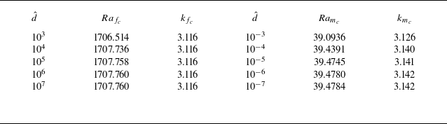
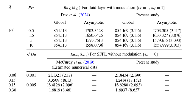
is reported in table 1. It can be observed from table 1 that the values of
 $Ra_{f_c}$
remain the same up to three decimal places for the values of
 $\hat {d} \geqslant 10^6$
. This value is considered the infinite limit of the depth ratio for all the computations reported here concerning a fluid-layer case. Further, the sensitivity analysis conducted to narrow down the parametric space for this case reveals the obvious results of
 $\alpha$
,
 $\hat {\kappa }$
and
 $G_m$
being non-significant parameters and thus are fixed to 0.1, 0.1 and 1, respectively. To validate the results, we refer to the investigation by Rosenblat & Tanaka (Reference Rosenblat and Tanaka1971), in which the authors considered a two-term Galerkin approximation resulting in
 ${\textit{Ra}}_{f_c} = 1728$
, apparently different from the exact value of 1707.762. The same holds for all other values of
 ${\textit{Ra}}_{f_c}$
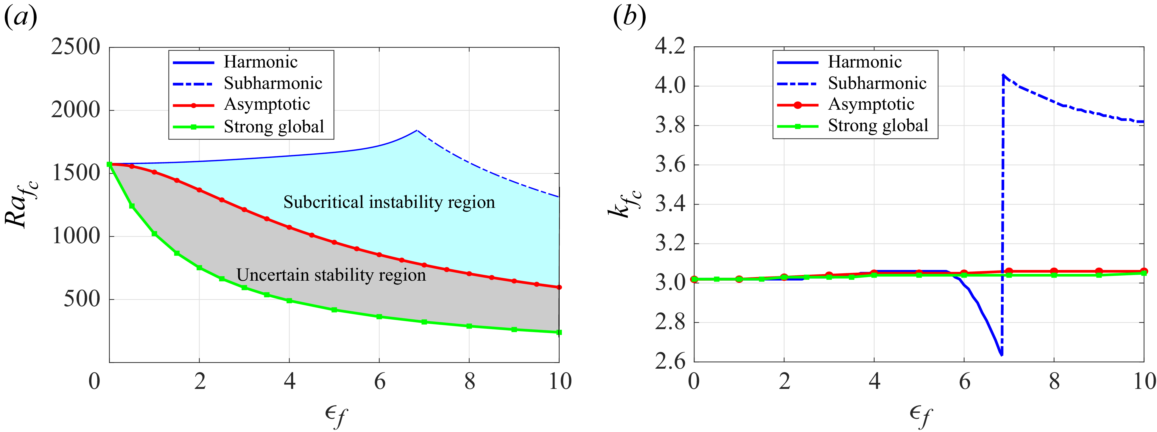
under modulation reported in Rosenblat & Tanaka (Reference Rosenblat and Tanaka1971). Therefore, the only possibility is to compare the present results qualitatively, using figure 2 and Rosenblat & Tanaka (Reference Rosenblat and Tanaka1971), figures 1 and 4. Figure 2(a) shows the variation in
 ${\textit{Ra}}_{f_c}$
and
 $k_{f_c}$
with modulation amplitude
 $\epsilon _{\!f}$
for
 $\omega _{\!f} = 20$
. For
 $\textit{Pr}_{\!f} = 1$
and small modulation amplitudes,
 ${\textit{Ra}}_{f_c}$
increases with
 $\epsilon _{\!f}$
. This conclusion aligns with the result mentioned by Rosenblat & Tanaka (Reference Rosenblat and Tanaka1971). Figure 2(b) shows the change in critical Rayleigh number with increasing modulation frequency for
 $\epsilon _{\!f} = 0.4$
. The curve corresponding to
 $\textit{Pr}_{\!f} = 1$
compares well with the result in Rosenblat & Tanaka (Reference Rosenblat and Tanaka1971), figure 1.
Critical Rayleigh number for the fluid domain and the porous domain (note that
 $\alpha = 0.1, \hat {\kappa } = 0.1, \sqrt {Da} = 0.002, \textit{Pr}_{\!f} = 7, \phi = 0.3, Bi = 10^6$
).

(a) Values of
 ${\textit{Ra}}_{f_c}$
and
 $k_{f_c}$
vs
 $\epsilon _{\!f}$
(solid, harmonic; dash-dotted, subharmonic) and (b)
 $ {\textit{Ra}}_{f_c}$
vs
 $\omega _{\!f}$
. Note that
 $\alpha = 0.1$
,
 $\hat {\kappa } = 0.1$
,
 $\sqrt {Da} = 0.002$
,
 $Bi = 10^6$
,
 $G_m = 1$
,
 $\hat {d} = 10^6$
,
 $\omega _{\!f} = 20$
,
 $\epsilon _{\!f} = 0.4$
, with
 $\textit{Pr}_{\!f}$
values shown on the panels.

While examining the accuracy of the analysis, we recognised that a few exciting results concerning convection in a fluid layer with a time-periodic temperature field should be reported, as none of the earlier studies documents those. The Rayleigh number, at which a constant adverse thermal gradient without modulation causes the convective motion, is altered to a higher value due to the formation of a time-dependent thermal boundary layer (TBL) due to modulation of the temperature near the lower plate. The variations in the gradients of this TBL are negligible for very small amplitudes, and thus its influence on the stability characteristics is minimal. Still, at higher amplitudes, temperature modulation results in higher temperature differences, forming a TBL with a substantial thermal gradient, affecting the onset of flow. For small values of
 $\epsilon _{\!f}$
, the TBL has a positive thermal gradient at the outset that changes to a negative one over the modulation period, resulting in a more stable conduction state. However, as
 $\epsilon _{\!f}$
increases, the magnitude of the thermal gradient increases, and the stabilisation effect becomes more significant. These observations are apparent in figure 2. We also notice that in figure 2(a) there are synchronous disturbances for the curve corresponding to
 $\textit{Pr}_{\!f} = 1$
until
 $\epsilon _{\!f} = 1.91$
. On increasing
 $\epsilon _{\!f}$
further, we encounter subharmonic instability, which is not mentioned in Rosenblat & Tanaka (Reference Rosenblat and Tanaka1971) as the authors had restricted their calculations to
 $\epsilon _{\!f} \leqslant 1$
. With a further increase in the modulation amplitude, the Rayleigh number for the occurrence of subharmonic instability decreases. This subharmonic instability sustains only until
 $\epsilon _{\!f} = 5.49$
; later, the harmonic instability reappears (for
 $\epsilon _{\!f} \geqslant 5.49$
). Interestingly, When
 $\epsilon _{\!f}$
surpasses approximately 6.1, the value of
 ${\textit{Ra}}_{f_c}$
for convective instability drops below the value of
 ${\textit{Ra}}_{f_c}$
at which convection starts in the no-modulation case, i.e. the temperature modulation has a destabilising effect, reported for
 $\epsilon _{\!f} \gt 6.1$
. Note that the
 $(\epsilon _{\!f}, {\textit{Ra}}_{f_c})$
-curve pattern coincides with those reported by Yih & Li (Reference Yih and Li1972). Large values of the Prandtl number lead to destabilisation, as shown in the
 $(\epsilon _{\!f}, {\textit{Ra}}_{f_c})$
-curve for the Prandtl number
 $\textit{Pr}_{\!f} = 7$
in figures 2(a) and 2(b). An increase in the fluid’s momentum diffusivity is due to a rise in the Prandtl number, which would decelerate the modulation’s stabilising effect. Since the momentum diffusivity of the fluid is high when
 $\textit{Pr}_{\!f} = 7$
, it induces a less effectual hindrance to the commencement of convection than in the case of
 $\textit{Pr}_{\!f} = 1$
. The disturbances with half of the forcing frequency appear for slightly greater values of modulation amplitude
 $(\epsilon _{\!f} \gt 3.95)$
when
 $\textit{Pr}_{\!f} = 7$
. The
 $(\epsilon _{\!f},k_{f_c})$
-curve agrees well with the published results by Bhadauria (Reference Bhadauria2002). The discontinuities in the curves show the jump from harmonic mode to subharmonic mode or vice versa. As the discontinuity point approaches, the critical wavenumber suffers a drastic change, representing the change in cell size. Figure 2(b) demonstrates the effect of modulation frequency
 $\omega _{\!f}$
on the value of
 ${\textit{Ra}}_{f_c}$
for modulation amplitude
 $\epsilon _{\!f} = 0.4$
and two different Prandtl numbers
 $\textit{Pr}_{\!f} = 1, 7$
with similar conclusions mentioned above.
4.1.2. Porous layer under modulation
When
 $\hat {d} \to 0$
, the fluid layer becomes very thin, reducing the system to a porous layer subjected to modulation. For the non-modulated problem (
 $\epsilon _m = 0$
), the critical Rayleigh numbers (
 ${\textit{Ra}}_{m_c}$
) for the porous-layer case corresponding to small values of
 $\hat {d}$
are mentioned in table 1. The values of the
 ${\textit{Ra}}_{m_c}$
do not vary up to 3 decimals for
 $\hat {d} \leqslant 10^{-6}$
, and thus, it is considered the limiting value of the depth ratio for the reported computations for instability in a porous layer. Moreover, results from the ANOVA test performed to reduce the parametric space for this case are apparent as
 $\alpha$
,
 $\hat {\kappa }$
and
 $\textit{Pr}_{\!f}$
are the non-significant parameters and thus fixed to 0.1, 0.1 and 7, respectively.
(a) Values of
 ${\textit{Ra}}_{m_c}$
and
 $k_{m_c}$
vs
 $\epsilon _m$
(solid, harmonic; dash-dotted, subharmonic) and (b)
 ${\textit{Ra}}_{m_c}$
vs
 $\omega _m$
. Note that
 $\alpha = 0.1$
,
 $\hat {\kappa } = 0.1$
,
 $\sqrt {Da} = 0.002$
,
 $Bi = 10^3$
,
 $\phi = 0.3$
,
 $G_m = 1$
,
 $ \textit{Pr}_{\!f} = 7$
,
 $\hat {d}= 10^{-6}$
.

We report the results of the periodic heating’s effect on the thermal instability in a porous domain in figure 3. The change in the critical Rayleigh number and wavenumber for the porous domain
 ${\textit{Ra}}_{m_c}, k_{m_c}$
with modulation amplitude
 $\epsilon _m$
for two different frequencies is obtained when
 $\hat {d} = 10^{-6}$
. The destabilising nature of modulation in figure 3(a) is the same as reported by Chhuon & Caltagirone (Reference Chhuon and Caltagirone1979), validating our analysis. Further, the appearance of subharmonic instability in the porous layer induced by thermal modulation of large amplitude (
 $\epsilon _m \gt 5.9$
) is observed when
 $\omega _m = 10$
. The curve corresponding to
 $\omega _m = 20$
demonstrates that increasing modulation frequency intensifies the destabilisation effect of the modulation amplitude on the commencement of thermal convection in a porous domain. However, for large
 $\epsilon _m$
values, the destabilising effect is more prominent when
 $\omega _m = 10$
, which shows the sensitivity of the layer to small frequencies. For large
 $\omega _m$
, subharmonic instability sets in the system for slightly higher amplitudes. The
 $k_{m_c}$
curves display discontinuous jumps at critical
 $\epsilon _m$
values for which instability mode shifts from harmonic to subharmonic. For large values of
 $\epsilon _m$
, the difference between the critical wavenumbers for
 $\omega _m = 10,$
and 20 is more prominent, representing a pronounced difference between cell sizes. The stability curve in the (
 $\omega _m, {\textit{Ra}}_{m_c}$
)-plane for three distinct modulation amplitudes is presented in figure 3(b). The curve obtained for
 $\epsilon _m = 1$
agrees with that in Chhuon & Caltagirone (Reference Chhuon and Caltagirone1979). Increasing frequency tends to destabilise the porous domain. The modulation effect is negligible when
 $\omega _m$
is large. The number of Chebyshev polynomials and Fourier modes needs to be increased in the case of small modulation frequencies to maintain the precision of the numerical results, which gives rise to the time complexity issue in the computation of eigenvalues. Thus, it is appropriate to mention that the technique used in the present study is not suitable for
 $\omega _m \lt \lt 1$
.
4.2. Stability of an SFPL system
The problems concerning SFPL are generally investigated either with a configuration in which the depth of the fluid layer is comparable to that of the porous layer or when a very shallow fluid layer is above a porous layer. The former assumption is more suitable for mathematical tractability, whereas the latter is more practical and exhibits an intricate dynamics in terms of stability and flow patterns due to the interaction of the fluid and solid, as well as capillary effects. This section reports these two cases under the considered hydrodynamic configuration involving modulated heating. In the first case, we assume that the fluid and porous layers have the same depths (
 $d_{\!f} = d_m$
). Corresponding results for the non-modulated case of this configuration have been discussed by Taslim & Narusawa (Reference Taslim and Narusawa1989). The same was utilised to verify that, following the present procedure, we could recover all the results reported in Taslim & Narusawa (Reference Taslim and Narusawa1989), table 5, precisely as the limiting case (
 $\epsilon _{f} = {0}$
) of the present analysis.
Further, considering the upper boundary to be isothermal (
 $Bi\gt \gt 1$
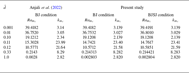
), a comparison of the results of the non-modulated problem for a range of depth ratios is made in table 2 with the results of Anjali et al. (Reference Anjali, Khan and Bera2022) wherein the stability of a Poiseuille flow in an SFPL system is studied using the commonly used BJ conditions at the interface. To accommodate the possibility of obtaining nonlinear bounds, we prefer to implement BJSJ conditions in our analysis, as mentioned earlier. With this intent, table 2 also includes a comparison between the instability limits produced by BJ and BJSJ interfacial conditions. The numerical results of the present study for the BJ condition, as evident by table 2, are in satisfactory agreement with those previously reported in Anjali et al. (Reference Anjali, Khan and Bera2022). Moreover, the
 ${\textit{Ra}}_{f_c}$
values at which instability sets in for the system are marginally higher for the BJSJ condition than those for the BJ condition, as the BJSJ condition neglects the porous domain velocity at the interface, resulting in mildly higher
 $({\lt}1\,\%)$
instability limits. We now proceed to discuss the results of the natural convection in SFPLs in two cases: (i)
 $\hat {d} = 1$
and (ii)
 $\hat {d} \lt 1$
.
Comparison of critical Rayleigh number for porous layer (note that
 $\alpha = 0.1, \hat {\kappa } = 0.7, \sqrt {Da} = 0.002, Bi = 10^4, \textit{Pr}_{\!f} = 7, G_m = 10, \epsilon _m = 0)$
.

4.2.1. When the fluid and the porous layers have equal depths
The effect of modulated heating on the commencement of RBC in a superposed system comprising layers of fluid and a porous medium having the same depth is depicted in figure 4. The modulation effect on
 ${\textit{Ra}}_{f_c}$
with varying
 $\epsilon _{\!f}$
in figure 4(a) is more significant for
 $\omega _{\!f} = 10$
than
 $\omega _{\!f} = 20$
, in stabilising or destabilising the system. The modulated temperature of low amplitudes tends to stabilise the system, and the instability onset exhibits harmonic oscillations. Destabilisation occurs for relatively large values of
 $\epsilon _{\!f}$
, and the subharmonic mode prevails at the onset of convection, as in the case of a clear fluid layer. The excitation of subharmonic instability occurs earlier for
 $\omega _{\!f} = 10$
than
 $\omega _{\!f} = 20$
, representing the fact that the system is sensitive to small frequencies due to the role of the TBL. The variation in
 $k_{f_c}$
with amplitude for
 $\hat {d} = 1$
is similar to that of
 $k_{f_c}$
for the fluid layer under modulation. It is evident that the external forcing frequency effectively regulates the onset of convection in an SFPL system. Figure 4(b) illustrates how
 ${\textit{Ra}}_{f_{c}}$
changes concerning
 $\omega _{\!f}$
for three distinct values of modulation amplitude, depicting the fact that, at low modulation frequencies, the TBL thickness is sufficiently large, resulting in stabilisation of the basic state, i.e. with an increase in
 $\epsilon _{\!f}$
,
 ${\textit{Ra}}_{f_c}$
increases. Nevertheless, the modulation effect turns insignificant for high modulation frequencies due to the boundary layer thickness approaching zero.
(a) Values of
 ${\textit{Ra}}_{f_c}$
and
 $k_{f_c}$
vs
 $\epsilon _{\!f}$
(solid, harmonic; dash-dotted, subharmonic), (b)
 ${\textit{Ra}}_{f_c}$
vs
 $\omega _{\!f}$
, (c) and (d) represent the streamlines and perturbation temperature in the
 $(x,z)$
plane at the onset of convection for
 $\epsilon _{\!f} = 6.84$
(harmonic flow) and
 $\epsilon _{\!f} = 6.85$
(subharmonic flow), respectively. Note that
 $\alpha = 0.1$
,
 $\hat {\kappa } = 0.1$
,
 $\sqrt {Da} = 0.002$
,
 ${Bi} = 10^3$
,
 $\textit{Pr}_{\!f} = 7$
,
 $\phi = 0.3$
,
 $G_m = 1$
,
 $\omega _{\!f}=20$
,
 $\hat {d} = 1$
.

The mode switch to subharmonic motions is an intriguing phenomenon like resonance and needs further insight. To understand the flow pattern and perturbed temperature distribution in the proximity of this mode switching, we plot the streamlines and perturbed thermal field in figure 4(c–d) when
 $\omega _{\!f} = 20$
. The streamlines and perturbed temperature profile at the onset of harmonic flow for the amplitude
 $\epsilon _{\!f} = 6.84$
are depicted in figure 4(c). In contrast, figure 4(d) represents streamlines and perturbed temperature profiles at the onset of subharmonic flow for the amplitude
 $\epsilon _{\!f} = 6.85$
. When the instability mode shifts from harmonic to subharmonic, there is an apparent difference in the cell size of the harmonic and subharmonic flow, with tall, thin convective cells appearing in the subharmonic flow, portraying large values of critical wavenumber. Moreover, the fluid mode dominates the convection in synchronous and subharmonic flows, with perturbed temperature cells developing only in the fluid domain. Overall, the stability of an SFPL system with equal depths subjected to modulated heating responds similarly to a fluid layer under modulation, except that the convective flow is in both layers, with fluid mode being dominant.
Figure 5 displays variations in the critical Rayleigh number
 ${\textit{Ra}}_{f_c}$
under different combinations of modulation parameters in the (
 $\epsilon _{\!f}, \omega _{\!f}, {\textit{Ra}}_{f_c}$
)-space and illustrates the range of modulation parameters for which the harmonic (plotted in blue) or subharmonic (plotted in red) mode of convection prevails. We observe that the convective motion prevails through the harmonic mode for small and large values of the modulation frequency and small values of the modulation amplitude. For moderate values of
 $\omega _{\!f}$
,
 ${\textit{Ra}}_{f_c}$
initially increases and reaches a maximum value, then decreases to fall below the
 ${\textit{Ra}}_{f_c}$
value corresponding to the no-modulation case with increasing
 $\epsilon _{\!f}$
. An exciting result is the existence of bicritical points for small values of
 $\omega _{\!f}$
, at which two harmonic waves with different wavenumbers are excited simultaneously (Hazra et al. Reference Hazra, Kumar and Mitra2020). The contour plot in the (
 $\epsilon _{\!f},\omega _{\!f}$
)-plane depicts the regions of harmonic and subharmonic instability for the modulation parameters. The colour legends at the top (representing
 ${\textit{Ra}}_{f_c}$
-values) may be referred to realise that darker regions indicate stabilisation, while brighter regions correspond to a destabilised system. The valleys with red contours represent the amplitude–frequency combinations that induce subharmonic instability.
Three-dimensional surface plot in the
 $\epsilon _{\!f} - \omega _{\!f} - {\textit{Ra}}_{f_c}$
space with contour plots in the (
 $\epsilon _{\!f},\omega _{\!f}$
)-plane for
 $\hat {d}=1$
(blue, harmonic; red, subharmonic). Note that
 $\alpha = 0.1$
,
 $\hat {\kappa } = 0.1$
,
 $\sqrt {Da} = 0.002$
,
 ${Bi} = 10^3$
,
 $\textit{Pr}_{\!f} = 7$
,
 $\phi = 0.3$
,
 $G_m = 1$
.

The effect of externally imposed thermal modulation depends on the existing system configuration represented by the physical parameters in the SFPL system. To reduce the parametric space and determine the modulation effect in systems of different configurations, a sensitivity analysis for SFPL systems with
 $\hat {d} = 1$
reveals
 $G_m$
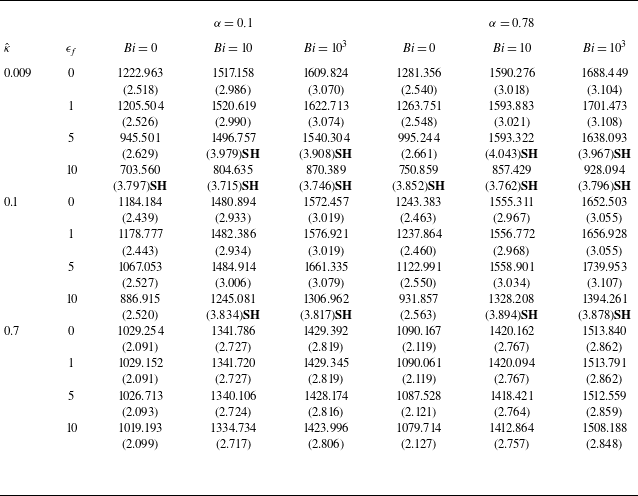
to be a non-significant parameter. Accordingly, we provide figure 6 and table 3, which report the impact of the modulation amplitude for significant parameters
 ${Bi}, \hat {\kappa }, \textit{Pr}_{\!f}$
and
 $\alpha$
, while
 $G_m$
is fixed to be 1. The stabilising effect of modulation is apparent in all the figures except in the case of Biot and Prandtl numbers. We discuss the findings one by one. As documented in the formulation, a mixed-type boundary condition governs the temperature at the upper surface in the present SFPL configuration, wherein the values of Biot number
 $\textit{Bi}$
decide the nature of the boundary. An adiabatic upper surface is assumed by selecting
 ${Bi} = 0$
, whereas large values of
 $\textit{Bi}$
mean an isothermal upper boundary. Figure 6(a) displays the influence of the Biot number
 $\textit{Bi}$
with modulation amplitude
 $\epsilon _{\!f}$
on the critical Rayleigh number
 ${\textit{Ra}}_{f_c}$
. The curves are plotted for different
 ${Bi}\hbox{-}$
values, ranging from zero to
 $10^3$
. Modulation stabilises the system for large
 $\textit{Bi}$
values due to the upper surface’s conducting nature. The heat loss from the upper surface and the increase in modulation amplitude delay the commencement of convection. The intensification of the stabilising effect is suppressed as
 ${Bi} \to 1000$
. Meanwhile, the modulation effect switches to destabilising the system for the insulating upper surface (
 ${Bi} = 0$
) as there is no heat loss from the upper surface. The adiabatic upper surface and the increasing modulation amplitude raise the heat transfer in the fluid domain, which causes the system to convect early, as apparent in figure 6(a).
Critical Rayleigh number
 ${\textit{Ra}}_{f_{c}}$
with critical wavenumber
 $k_{f_{c}}$
when
 $\phi = 0.3$
,
 $\omega _{\!f} = 20$
,
 $\hat {d} = 1$
,
 $\textit{Pr}_{\!f} = 7$
,
 $G_m = 1$
,
 $\sqrt {Da} = 0.002$
. The
 $Ra_{f_c}(k_{f_c})$
values with SH represent subharmonic instability mode.

Variation of
 ${\textit{Ra}}_{f_{c}}$
with
 $\epsilon _{\!f}$
for different values of (a) Biot numbers, (b) ratio of thermal diffusivities (solid, harmonic; dash-dotted, subharmonic), (c) Prandtl numbers, (d) BJ constants. Fixed values of the parameters are
 $\omega _{\!f} = 20$
,
 $\alpha = 0.1$
,
 $\hat {\kappa } = 0.1,$
 $\sqrt {Da} = 0.002$
,
 ${Bi} = 10^3$
,
 $\phi = 0.3$
,
 $\hat {d} =1$
,
 $\textit{Pr}_{\!f} = 7$
,
 $G_m = 1$
.

Thermoconvective instability in a porous layer gets delayed when the thermal diffusivity of the fluid is significantly lower compared with the effective thermal diffusivity of the porous domain. Quicker heat diffusion in the porous layer smooths out the thermal gradient, resulting in a stable layer. In an SFPL system, the diffusion of heat through the interface to the fluid layer fails to build a sufficient thermal gradient in the fluid layer due to the low thermal diffusivity of the fluid. Transient heating (and cooling) of the lower surface due to modulation further decelerates the process. Consequently, the application of modulated temperature of small amplitudes tends to stabilise the system effectively, as in the case of
 $\hat {\kappa } = 0.009$
, reported in figure 6(b). For moderate values of
 $\epsilon _{\!f}$
, the instability mode shifts to subharmonic due to lag in the thermal response of the fluid of low diffusivity. The system’s response changes radically in subharmonic mode, and it gets destabilised by further increasing the amplitude. Note further that the stabilising effect of modulation becomes less pronounced due to the increased thermal diffusivity of the fluid for the case of larger values of
 $\hat {\kappa } (\hat {\kappa } = 0.1)$
. Significantly large values of
 $\hat {\kappa }$
decrease the Rayleigh number for the fluid layer, which is not instantly visible in figure 6(b) but can be observed in the quantitative results reported in table 3. Note that
 $k_{f_c}$
increases when the instability mode switches from the harmonic to the subharmonic mode (see table 3), and cells in subharmonic convection are thinner and taller than those in the harmonic mode.
The role of the Prandtl number in the instability criteria is depicted graphically in figure 6(c). Small Prandtl numbers (
 $\textit{Pr}_{\!f}$
) indicate a fluid layer with high thermal diffusivity, implying faster heat conduction, resulting in a stable layer. Consequently, the curve corresponding to
 $\textit{Pr}_{\!f} = 5$
displays the most significant stabilising effect induced by external modulation of various amplitudes. For large values of
 $\textit{Pr}_{\!f}$
, the modulation effect is reversed as a low diffusivity leads to a build-up of strong gradients across the layer, destabilising the system.
Figure 6(d) exhibits the impact of
 $\alpha$
and
 $\epsilon _{\!f}$
on the commencement of convection in SFPL. The practical values of the BJ constant (
 $\alpha$
) for various metal foams and Aloxite (Straughan Reference Straughan2002) are considered in the present analysis. The non-modulated critical Rayleigh number
 ${\textit{Ra}}_{f_c}$
grows in response to a higher value of
 $\alpha$
. Similar to the non-modulation case, the Rayleigh number increases with an increase in
 $\alpha$
for the range of
 $\epsilon _{\!f}$
values. However, the stabilising effect of modulation is found to be insensitive to the variations in
 $\alpha$
. We now discuss the case of an SFPL system in which the fluid layer is much thinner than the porous layer.
4.2.2. When the fluid layer’s depth is relatively smaller than that of the porous layer
An interesting case of SFPL systems is when the upper fluid layer is thin compared with the porous layer, as is the case of water layers on sediments. In this case, the interfacial region becomes the primary activity zone, leading to patterns and intricacies that do not exist in the previous case of layers with equal/comparable depths. Chen & Chen (Reference Chen and Chen1988) observed the bimodal behaviour and demonstrated that the shifting of instability modes from porous mode to fluid-layer mode happens with a change in the depth ratio. The system’s dynamics changes with an increase in
 $\hat {d}$
from 0.10 to 0.11, and the fluid layer dominates the convection when
 $\hat {d} = 0.11$
. This change in the system’s dynamics can also happen due to variations in other parameters, namely
 $\hat {\kappa }$
and
 $Da$
, that represent the material properties (Han et al. Reference Han, Wang and Wang2020; McCurdy et al. Reference McCurdy, Moore and Wang2022). Obviously, changing these properties requires altering the system completely. In contrast, the present analysis illustrates a way to induce the mode shift phenomenon in the SFPL system without changing its intrinsic properties, which is applying a modulating temperature field to the porous bed underlying a fluid domain so that the fluid mode dominates the convection even when
 $\hat {d} \lt 0.1054$
, which is the predicted critical value of depth ratio in McCurdy et al. (Reference McCurdy, Moore and Wang2022). Figure 7(a) presents the integrated effect of the depth ratio and modulation amplitude on the commencement of thermal convection in an SFPL system for small values of
 $\hat {d}$
. The solid and dotted parts of the stability curves denote the preferred convection mode, i.e. porous and fluid, respectively. A conventional destabilisation effect on a porous layer is reported due to the application of modulation for all the
 $\hat {d}$
values chosen here. The mode shifting occurs for a small
 $\epsilon _m$
when
 $\hat {d} = 0.1$
, whereas, for
 $\hat {d} = 0.09$
, the same occurs at a large
 $\epsilon _m$
. This indicates that, the smaller the
 $\hat {d}$
is, the larger the required
 $\epsilon _m$
is for convection to be dominated by the fluid domain. The plots of
 $k_{m_c}$
show discontinuities, indicating the shifts in the instability mode from porous to fluid. The wavelength decreases drastically at these discontinuities. A higher value of
 $k_{m_c}$
represents the fluid mode as the preferred convection mode.
(a) Variations in
 ${\textit{Ra}}_{m_c}$
and
 $k_{m_c}$
with variation in
 $\epsilon _m$
(solid, porous mode; dotted, fluid mode), (b) and (c) represent the streamlines and perturbation temperature at the onset of convection with
 $\hat {d} = 0.10$
for
 $\epsilon _m = 1$
(porous mode), and
 $\epsilon _m = 2$
(fluid mode), respectively. Note that
 $\alpha = 0.1$
,
 $\hat {\kappa } = 0.7$
,
 $\sqrt {Da} = 0.002$
,
 $Bi = 10^3$
,
 $\phi = 0.3$
,
 $G_m = 1$
,
 $\textit{Pr}_{\!f} = 7$
.

Table 4 reports the Rayleigh number and wavenumber corresponding to porous and fluid modes, respectively, for two distinct
 $\hat {d}$
. In the case of
 $\hat {d} = 0.10$
, the instability onset at
 $\epsilon _m = 1$
is prominent in the porous domain since the Rayleigh number corresponding to the low wavenumber range is smaller than that corresponding to the high wavenumber range. While for
 $\epsilon _m = 2$
, the instability is dominated by the fluid layer. The change in the
 $Ra_{m_c}$
is because of the change in the critical wavenumber for the porous medium, which is displayed in table 4.
Rayleigh number (
 ${\textit{Ra}}_{m}$
) and wavenumber (
 $k_{m}$
) for porous layer with
 $\omega _m = 20$
,
 $\alpha = 0.1$
,
 $\textit{Pr}_{\!f} = 7$
,
 $\sqrt {{Da}} = 0.002$
,
 ${Bi} = 10^3$
,
 $\hat {\kappa } = 0.7$
,
 $G_m = 1$
,
 $\phi = 0.3$
.

To comprehend the mechanism of mode shifting for
 $\hat {d} = 0.10$
, we examine figures 7(b) and 7(b), representing the patterns of streamlines and perturbed temperature as the background at the onset of convection. Figure 7(b) is obtained for
 $\epsilon _m = 1$
by scaling the critical wavelength of eigenfunctions in the fluid layer such that the wavelength in both domains is the same. The porous mode is the most unstable for
 $\epsilon _m = 1$
(see table 4); for the low wavenumber values (
 $k_m = 2.167$
),
 ${\textit{Ra}}_{m_c}$
is minimal, and the porous layer will dominate convection. The same is evident from the figure, as the cells’ formation is in the whole domain. The perturbation temperature distribution displays a downward plume at the centre of the cell, which was also reported by Chen & Chen (Reference Chen and Chen1992). The perturbed temperature profile also shows a standard convection pattern. Figure 7(c) is obtained for
 $\epsilon _m = 2$
, having a similar setting as for figure 7(b). In this instance, the fluid layer dominates the convection as the convection cells in the fluid domain are pronounced compared with those in the porous domain.
In table 4, the fluid-layer mode is the most unstable mode for
 $\epsilon _m = 2$
, as for the large values of wavenumber (
 $k_m = 28.67$
), the Rayleigh number is minimum. Therefore, modulation can effectively control the convection mode without altering the system configuration, i.e. for an SFPL system with
 $\hat {d} \sim 0.1$
, temperature modulation can govern whether the convection is dominant in the fluid or porous layer. The result offers practical value in heat transfer applications where structural modifications to the system are either constrained or costly.
Further, to make the present analysis thorough, the critical values of modulation amplitude
 $\epsilon _{m_c}$
, at which porous mode-dominated convection transitions to the fluid mode-dominated regime, are determined for various SFPL systems from the studies that observed similar transitions by varying
 $\hat {d}$
. We fix
 $Bi = 10^5$
to have an isothermal upper surface of the fluid layer, and the frequency of the modulation
 $\omega _m = 20$
. The chosen studies in table 5 (Chen & Chen Reference Chen and Chen1988; Straughan Reference Straughan2002; Hirata et al. Reference Hirata, Goyeau, Gobin, Carr and Cotta2007; Yin, Fu & Tan Reference Yin, Fu and Tan2013; Han et al. Reference Han, Wang and Wang2020) employ the two-domain approach and Darcy’s law for the fluid flow in the SFPL system, which is in line with the present investigation. Table 5 presents the critical modulation amplitude
 $\epsilon _{m_c}$
and corresponding
 $Ra_{m_c}$
and
 $k_{m_c}$
for depth ratios less than the predicted depth ratios by McCurdy et al. (Reference McCurdy, Moore and Wang2022) for the SFPL systems chosen in various previous studies. Note that the values of a few parameters (not specified in the source article) are chosen appropriately to find
 $\epsilon _{m_c}$
. Naturally, altering these parameters will modify the critical values reported in the table. The intent is to demonstrate that modulation can induce mode shift. Note that, at the onset of instability, the flow regime may be either synchronous or subharmonic. In particular, for large values of
 $G_m$
, the flow regime is subharmonic, characterised by a smaller cell size.
Critical modulation amplitude
 ${\epsilon _m}_c$
and corresponding
 $Ra_{m_c} (k_{m_c})$
for various SFPL systems with
 $\omega _m = 20$
,
 ${Bi} = 10^5$
. (Values with SH represent subharmonic instability mode.)

We conclude the analysis of this case by examining various SFPL configurations with a fixed
 $\hat {d} = 0.1$
. An ANOVA test reveals that the parameters
 $\alpha$
and
 $\textit{Pr}_{\!f}$
are statistically non-significant and thus we set
 $\alpha = 0.1$
, and
 $\textit{Pr}_{\!f} = 7$
. We now embark on the effect of modulation for different
 $\textit{Bi}$
,
 $\hat {\kappa }$
,
 $G_m$
and
 $\omega _m$
with
 $\hat {d} = 0.1$
, as depicted in figure 8(a–d). The effect of modulation is to destabilise the system for all
 $\textit{Bi}$
values (see figure 8
a). However, the intensity of the destabilisation can be controlled by varying
 $\textit{Bi}$
. For
 $Bi = 0$
, the influence of modulation is weak, and instability arises exclusively through the porous mode, since only a weak thermal gradient can develop in the fluid layer for an insulating wall. As
 $\textit{Bi}$
increases, the destabilisation effect becomes more pronounced, the thermal gradient becomes sufficient in the fluid layer and the onset mode switches from porous to fluid due to periodic heating. In the presence of modulation, the monotonic effect of
 $\textit{Bi}$
changes to a non-monotonic one as
 $Ra_{m_c}$
values for
 $Bi = 1000$
are less than those for
 $Bi = 1$
when the amplitude surpasses approximately 3.5. Figure 8(b) represents the combined effect of the thermal diffusivity ratio and modulation amplitude on the convective instability in the SFPL system with
 $\hat {d} = 0.1$
. For small values of
 $\hat {\kappa }$
, the effect of modulation is stabilising but very ineffective and convective instability arises through the porous mode only. For
 $\hat {\kappa } = 0.1$
,
 $\kappa _{\textit{eff}}$
is higher than
 $\kappa _{\!f}$
, resulting in a rapid heat diffusion in the porous domain, which counters the effect of periodic heating, and a seemingly ineffective stabilising effect appears. Moreover, this diffusion is inadequate for the fluid mode to prevail as a sufficient thermal gradient does not form in the fluid layer. For a slightly higher value of
 $\hat {\kappa }$
the heat diffusion slows down in the porous domain, thus
 $Ra_{m_c}$
is higher. In contrast, it quickens in the fluid layer and as a modulating temperature field of sufficiently large amplitude supervenes, the mode switches from porous to fluid mode. When
 $\hat {\kappa } = 1$
, the heat diffusivity is the same in both domains; the effect of modulation is destabilising with porous mode as the most unstable mode.
Variation of critical Rayleigh number
 ${\textit{Ra}}_{m_{c}}$
with modulation amplitude
 $\epsilon _m$
for different values of (a) Biot numbers, (b) ratio of thermal diffusivities, (c) ratio of specific heats, (d) modulation frequencies. Fixed values of the parameters are
 $\hat {d} =0.1$
,
 ${Bi} = 10^3$
,
 $\hat {\kappa } = 0.7$
,
 $G_m = 1$
,
 $\omega _m = 20$
,
 $\alpha = 0.1$
,
 $\sqrt {Da} = 0.002$
,
 $\phi = 0.3$
,
 $\textit{Pr}_{\!f} = 7$
.

The combined effect of specific heat ratio and modulation is depicted in figure 8(c). Modulation tends to destabilise the SFPL system; moreover, this effect is more pronounced for
 $G_m = 1$
and as
 $G_m$
increases, the destabilising effect becomes less effective. For a large value of
 $G_m$
, a large amount of heat is required for heat transfer in the porous domain, while the fluid layer experiences an effective heat transfer. However, the heat transfer from porous to fluid through the interface is slow, resulting in increased
 $Ra_{m_c}$
and a less pronounced destabilising effect. The assumed sinusoidally varying temperature applied on the lower wall is governed by two parameters: modulation amplitude and modulation frequency. Until now, only the amplitude’s effect on instability has been investigated. For completeness, figure 8(d) is presented to probe the combined effect of both modulation parameters. Changing the modulation frequency can change the critical amplitude value at which the mode shift occurs. In the porous mode regime,
 $Ra_{m_c}$
is insensitive to changes in
 $\omega _m$
, while in the fluid mode regime,
 $Ra_{m_c}$
values increase as frequency increases. This is due to the fact that the thermal gradient in the fluid layer weakens as
 $\omega _m$
grows, but strengthens for an increasing
 $\epsilon _m$
. Consequently, the critical
 $\epsilon _m$
increases with
 $\omega _m$
.
4.3. Comparison between linear and nonlinear results
Before comparing linear and nonlinear results, we validate the results obtained from the energy stability method in the limiting cases of the fluid layer with modulation and the SFPL without modulation. First, the results of a fluid layer under modulation can be obtained by taking a large value of
 $\hat {d}$
using the present model, which is then validated with those published by Dev et al. (Reference Dev, Suthar and Siddheshwar2024) in table 6. We note that the thresholds for strong global stability calculated from the present analysis are higher, and asymptotic threshold values are lower than the ones published in Dev et al. (Reference Dev, Suthar and Siddheshwar2024), which signifies that the present method yields a smaller uncertain stability region. The results for the limiting case of an SFPL system without modulation can be obtained by taking
 $\epsilon _m = 0$
and validated with those reported by McCurdy et al. (Reference McCurdy, Moore and Wang2019) in table 6. In their study, only graphical results are presented, and hence, we have estimated numerical values from McCurdy et al. (Reference McCurdy, Moore and Wang2019), figure 2. The threshold for strong global stability through the present analysis is higher than the estimated values from the published results. Note that the bounds through the energy stability method are always lower than those of linear instability analysis.
Validation of results of the energy method. Note that
 $ \alpha = 0.1$
,
 $\hat {\kappa }= 0.7$
,
 $\sqrt {{Da}} = 0.002$
,
 $\textit{Pr}_{\!f} = 7$
,
 $G_m = 1$
,
 ${Bi} = 10^6,$
 $\phi = 0.3$
.

Now, a comparison between linear and nonlinear (both asymptotic and strong global) thresholds for the Rayleigh number and wavenumber varying with modulation amplitude is presented for two different configurations of SFPL systems with
 $\hat {d} = 1$
and 0.1 in figures 9 and 10, respectively. It is evident from both figures that the thresholds obtained through the energy method are lower than the ones obtained through the linear theory; this raises the possibility of subcritical instability. There is a stark contrast between low and high modulation amplitudes in the case of linear stability. However, energy bounds (both asymptotic and strong global) do not display drastic changes when varying the modulation amplitude.
Variation in (a)
 ${\textit{Ra}}_{f_c}$
, and (b)
 $k_{f_c}$
with variation in
 $\epsilon _{\!f}$
for
 $\hat {d} = 1$
. Note that
 $\omega _{\!f}=20$
,
 $\alpha = 0.1$
,
 $\hat {\kappa } = 0.1$
,
 $\sqrt {{Da}} = 0.002$
,
 ${Bi} = 10^3$
,
 $\textit{Pr}_{\!f} = 7$
,
 $\phi = 0.3$
,
 $G_m = 1$
.

Variation in (a)
 ${\textit{Ra}}_{m_c}$
, and (b)
 $k_{m_c}$
with variation in
 $\epsilon _m$
for
 $\hat {d} = 0.1$
. Note that
 $\omega _m=20$
,
 $\alpha = 0.1$
,
 $\hat {\kappa } = 0.7$
,
 $\sqrt {{Da}} = 0.002$
,
 ${Bi} = 10^3$
,
 $\textit{Pr}_{\!f} = 7$
,
 $\phi = 0.3$
,
 $G_m = 1$
.

Figure 9(a) displays the change in
 ${\textit{Ra}}_{f_c}$
with a change in
 $\epsilon _{\!f}$
for
 $\hat {d} = 1$
corresponding to three stability criteria, namely linear, asymptotic and strong global. As discussed earlier, the linear instability can arise through the harmonic or subharmonic mode and
 ${\textit{Ra}}_{f_c}$
increases for a harmonic response, whereas it decreases for a subharmonic response. On the other hand, the value of
 ${\textit{Ra}}_{f_c}$
for nonlinear stability decreases for the whole range of
 $\epsilon _{\!f}$
. However, the rate of decrease of
 ${\textit{Ra}}_{f_c}$
with
 $\epsilon _{\!f}$
is different in asymptotic and strong global bounds, being more significant in the latter. It can be observed that the
 ${\textit{Ra}}_{f_c}$
value for all three limits is the same in the no-modulation case (
 $\epsilon _{\!f} = 0$
), which indicates that the possibility of subcritical instabilities stems from the modulating temperature field. This verifies the earlier reported results by Hill & Straughan (Reference Hill and Straughan2009) and McCurdy et al. (Reference McCurdy, Moore and Wang2019) that the energy stability bounds are roughly the same as linear instability bounds for RBC in an SFPL. The variation in the critical wavenumber with
 $\epsilon _{\!f}$
for the three criteria of stability are depicted in figure 9(b). It is observed that, for a critical
 $\epsilon _{\!f}$
, where the instability mode shifts from synchronous to subharmonic flow,
 $k_{f_c}$
for linear instability suffers significant changes depicting a difference in cell size for both flows. There is no critical value of
 $\epsilon _{\!f}$
in the values of strong global and asymptotic thresholds for which the system changes radically. For nonlinear stability criteria,
 $k_{f_c}$
show a monotonic increasing behaviour throughout the range of
 $\epsilon _{\!f}$
, while this was not the case for linear instability criterion due to the appearance of subharmonic mode.
Figures 10(a) and 10(b) display the effect of modulation on
 ${\textit{Ra}}_{m_c}$
and
 $k_{m_c}$
obtained from linear and nonlinear stability analyses for an SFPL system with
 $\hat {d} = 0.1$
. The linear instability can prevail through porous or fluid modes as a response to the sinusoidally varying temperature field, which symbolises convection occurring primarily in the whole or fluid domains, respectively. This type of response was not observed through energy stability analysis when analysing the effects of modulation, while in the absence of modulation, the occurrence of fluid mode was observed through both the analyses at roughly the same wavenumber (see table 6). However, similar to the case of
 $\hat {d} = 1$
, the subcritical instabilities are possible due to modulation. For the small range of
 $\epsilon _m$
, the nonlinear thresholds decay rapidly. This decay in
 ${\textit{Ra}}_{m_c}$
values slows down for large values of
 $\epsilon _m$
, illustrating the systems’ sensitivity toward small amplitude modulation.
Hill & Straughan (Reference Hill and Straughan2009) found that the linear instability theory is enough to study the classical RBC in an SFPL system as the subcritical region was very small. The present study also found a very small subcritical region for
 $\hat {d} = 0.1$
in no-modulation case, i.e. classical RBC in SFPL, which is tabulated in table 7. The quantitative results for
 $\hat {d} = 1$
are also presented. The linear and nonlinear thresholds are the same in the absence of modulation. On increasing the amplitude of periodic heating applied at the bottom, the subcritical region grows as linear and nonlinear thresholds are no longer the same or roughly the same. We summarise the significant findings of the present analysis in the next section.
Critical Rayleigh number (wavenumber) for linear, asymptotic and strong global stability when
 $\alpha = 0.1$
,
 $\textit{Pr}_{\!f} = 7$
,
 $\sqrt {{Da}} = 0.002$
,
 ${Bi} = 10^3, G_m = 1, \phi = 0.3$
. Values with SH represent subharmonic instability mode.

5. Conclusions
The present study investigates the role of time-periodic heating in regulating natural convection in SFPL systems confined between a rigid and an impermeable boundary. An experimentally validated two-domain approach is adopted to model the system. Two complementary stability frameworks – linear theory and the energy method – were implemented to determine the stability thresholds to characterise the system’s stability behaviour. From a modelling perspective, the present study has the advantage that it serves as a unified approach to extracting the results of the clear fluid case of RBC and its porous-layer analogue Darcy–Bénard convection under modulation of boundary temperatures. Building on this feature and the conclusions of earlier studies, we examined four representative SFPL configurations, characterised by the depth ratio
 $\hat {d}$
, while maintaining a fixed porous medium structure suitable for experimental realisation. Fixing the medium’s parameters partially addresses the complexity associated with the high-dimensional parametric space of the system. To resolve the issue further, an ANOVA-based sensitivity analysis was performed to screen other physical parameters in the four configurations.
The first two configurations represent the limiting cases of the fluid and porous layers, thereby contributing to the validation of results. In the case of a fluid layer, the critical Rayleigh number can have different variation patterns for small and large
 $\epsilon _{\!f}$
ranges. However, in the porous-layer case,
 $Ra_{m_c}$
shows decreasing behaviour for the whole range of modulation amplitude. Moreover, the instability onset with subharmonic oscillations is reported in the porous and fluid layers. The third SFPL configuration, corresponding to equal depths of the fluid and porous layers
 $(\hat {d} = 1)$
, exhibits characteristics identical to those of a fluid layer under modulation. Further, we can control the effect of modulation with the proper combination of physical parameters
 $\textit{Bi}$
,
 $\hat {\kappa }$
,
 $\textit{Pr}_{\!f}$
and
 $\alpha$
. Specifically, the parameters
 $\textit{Bi}$
and
 $\textit{Pr}_{\!f}$
can change the effect of modulation from stabilisation to destabilisation for small values of modulation amplitude.
In contrast to the existing results concerning the shift in the dominant convection mode in SFPL systems with
 $\hat {d} \sim 0.1$
, the present study found a way to restrict the instability region in the fluid or whole domain by simply applying the modulation instead of modifying the system. It is the first time such a result has been reported concerning SFPL systems. Obviously, the control of mode (porous or fluid) of instability in the SFPL system via modulation is sensitive to the other parameters
 $\textit{Bi}$
,
 $\hat {\kappa }$
,
 $G_m$
and
 $\omega _m$
. Another notable interesting result obtained through nonlinear analysis is the possibility of subcritical instabilities arising from periodic heating, indicating potential convective motion at lower temperature differences. Overall, the present study demonstrates the potential of temperature modulation as an external mechanism to regulate convective motions in superposed fluid–porous systems, which can be utilised in thermal management and geophysical processes. It is worth noting that extending the present investigation to examine Marangoni effects and boundary asymmetries could be of significant importance for practical applications involving porous convection with surface tension effects (Nield Reference Nield2009).
Acknowledgements
The authors are grateful to the reviewers and the editor, whose comments significantly improved the manuscript. The authors sincerely appreciate the guidance and inputs of Professor Pradeep G. Siddheshwar, Christ University, Bengaluru, India, and the kind assistance of Dr Kapil Dev, postdoctoral researcher, IITK, India. The authors also thank MNIT Jaipur for providing research facilities.
Declaration of interests
The authors report no conflict of interest.
Appendix A. Expressions for
 $\bar {\boldsymbol{T}}_{\boldsymbol{0}}$
and
$\tilde {\boldsymbol{T}}_{\boldsymbol{0}}$


 \begin{align} \bar {T}_0 &= \frac {\kappa _{\!f}d_mT_U + \kappa _{\textit{eff}} d_{\!f}T_L}{\kappa _{\!f}d_m + \kappa _{\textit{eff}} d_{\!f}}, \end{align}
 \begin{align} \tilde {T}_0 &\!=\! \frac {\Delta T}{{\textit{Pr}}_{\!f}(\bar {T}_0 - T_U)} {\text{Re}} \! \left (\! \frac {\sqrt {G_m}A(\omega _{\!f})}{\sqrt {G_m}A(\omega _{\!f}) \cosh \sqrt {\text{i}\omega _mG_m} + \sqrt {\hat {\kappa }}B(\omega _{\!f})\sinh \sqrt {\text{i}\omega _mG_m}} e^{\text{i} \omega _{\!f} t_{\!f}} \! \right ) \nonumber \\ &\!=\! \frac {\Delta T}{{\textit{Pr}}_m(T_L - \bar {T}_0 )} {\text{Re}} \! \left (\! \frac {\sqrt {G_m}A(\omega _{\!f})}{\sqrt {G_m}A(\omega _{\!f}) \cosh \sqrt {\text{i}\omega _mG_m} + \sqrt {\hat {\kappa }}B(\omega _{\!f})\sinh \sqrt {\text{i}\omega _mG_m}} e^{\text{i} \omega _m t_m}\! \right )\!, \end{align}
where
 $A(\omega _{\!f}) = Bi \sinh \sqrt {\text{i}\omega _{\!f}} + \sqrt {i\omega _{\!f}} \cosh \sqrt {\text{i}\omega _{\!f}}$
and
 $B(\omega _{\!f}) =\sqrt {i\omega _{\!f}} \sinh \sqrt {\text{i}\omega _{\!f}} + Bi \cosh \sqrt {\text{i}\omega _{\!f}}$
.
Appendix B. Expressions for
$\boldsymbol {f(z_{\!f})}$
and
$\boldsymbol{g(z_m)}$


 \begin{align} f(z_{\!f}) &= \dfrac {\sqrt {G_m}(A(\omega _{\!f})\cosh {(\sqrt {\text{i}\omega _{\!f}}z_{\!f})} - B(\omega _{\!f})\sinh {(\sqrt {\text{i}\omega _{\!f}}z_{\!f})})}{\sqrt {G_m}A(\omega _{\!f}) \cosh \sqrt {\text{i}\omega _mG_m} + \sqrt {\hat {\kappa }}B(\omega _{\!f})\sinh \sqrt {\text{i}\omega _mG_m}}, \end{align}
 \begin{align} g(z_m) &= \frac {\sqrt {G_m}A(\omega _{\!f})\cosh (\sqrt {\text{i}\omega _m}z_m) -\sqrt {\hat {\kappa }} B(\omega _{\!f})\sinh (\sqrt {\text{i}\omega _m}z_m)}{\sqrt {G_m}A(\omega _{\!f}) \cosh \sqrt {\text{i}\omega _mG_m} + \sqrt {\hat {\kappa }}B(\omega _{\!f})\sinh \sqrt {\text{i}\omega _mG_m}}. \end{align}