



1 Introduction
Minimal submanifolds are critical points of the volume functional among all compactly supported variations. More precisely, let
 $\Sigma ^k$
be a k-dimensional submanifold of some Riemannian ambient space
 $\overline {M}$
. We say that
 $\Sigma ^k$
is minimal if for every
 $p\in \Sigma $
, there is a neighborhood
 $U_p$
of p in
 $\Sigma $
such that
 $U_p$
minimizes the k-dimensional volume among all of its smooth variations with the fixed boundary
 $\partial U_p$
. This is equivalent to the condition of vanishing mean curvature. Let
 $\Sigma ^k$
be a compact manifold with boundary with the unit outer normal vector field
 $\eta $
on
 $\partial \Sigma ^k$
. We say that an isometric immersion
 $\Phi : \Sigma ^k\rightarrow \overline {M}$
is a free boundary minimal immersion (FBMI for short) if it is a critical point of the volume functional,
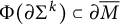 $\Phi (\partial \Sigma ^k)\subset \partial \overline {M}$
, and the image of
 $\eta $
is perpendicular to
 $\partial \overline {M}$
.
In the case where the ambient space
 $\overline {M}$
is the closed unit ball in the Euclidean space
 $\mathbb {E}^{m+1}$
, FBMIs have a nice description. Namely, all coordinate functions
 $\phi _i=x_i\circ \Phi $
,
 $i=0,\dots ,m$
, are Steklov eigenfunctions with the eigenvalue
 $\sigma =1$
, i.e., they are harmonic functions on
 $\Sigma ^k$
, and
 $\dfrac {\partial \phi _i}{\partial \eta }=\phi _i$
on
 $\partial \Sigma ^k$
. There is a similar description of FBMIs in the case that the ambient space
 $(\overline {M},\overline g)$
is a closed ball in a space of constant curvature, which is also the focus of this article.
We consider the standard upper unit hemisphere
 $\mathbb {S}^m_+$
in
 $\mathbb {E}^{m+1}$
and also the Lobachevsky m-space
 $\mathbb {H}^m$
as the hyperboloid in the Minkowski space
 $\mathbb {M}^{1,m}$
. When
 $(\overline {M},\overline g)$
is a suitably placed geodesic ball in
 $\mathbb {S}^m_+$
or in
 $\mathbb {H}^m$
, a map
 $\Phi :(\Sigma ^k,g)\rightarrow M$
is an FBMI if and only if the coordinate functions
 $\phi _i$
are solutions to the Robin problem. Namely, they satisfy the following system of equations:
 $$ \begin{align} \begin{cases} \Delta_g \phi_i= \lambda \phi_i&\text{ in}\, \Sigma,\\ \dfrac{\partial \phi_i}{\partial \eta}=\sigma \phi_i &\text{ on} \,\partial\Sigma, \end{cases} \end{align} $$
for suitably prescribed values of
 $\lambda $
and
 $\sigma $
. For example, in Sections 2 and 3, we consider situations in which
 $\lambda $
is prescribed and the corresponding
 $\sigma $
’s form a discrete sequence depending on
 $\lambda $
. Conversely, in Section 4, we prescribe
 $\sigma $
and let the
 $\lambda $
’s depend on
 $\sigma $
. In this article, we take the sign convention of the Laplace operator to be
 $\Delta _g=-\operatorname {div}_g\circ \nabla ^g$
. The existence of FBMI into geodesic balls in
 $\mathbb {S}^m_+$
or in
 $\mathbb {H}^m$
corresponds to the case where solutions of a system of the type (1.1) exist and form an isometric immersion into the respective ambient space (see [Reference Lima and Menezes26, Reference Medvedev28]). More generally, when the map
 $\Phi $
is just an immersion (not necessarily isometric), the coordinate functions are solutions of this system if and only if
 $\Phi $
is harmonic. In this case,
 $\Phi $
is a free boundary harmonic map (FBHM for short).
In order to find the metrics induced by FBMIs in geodesic balls in
 $\mathbb {S}^m_+$
and
 $\mathbb {H}^m$
, we characterize them as critical points of certain functionals. Let us recall the definition (see [Reference El Soufi and Ilias7, Reference Karpukhin and Metras18, Reference Nadirashvili29]).
Definition 1.1 Let g be a metric on a manifold
 $\Sigma ^k$
, and let F be a functional defined on some set
 $\mathcal {S}(\Sigma ^k)$
of metrics on
 $\Sigma ^k$
containing g. We say that g is an extremal metric for F if for all one-parameter smooth family metrics
 $g(t)$
in
 $\mathcal {S}(\Sigma ^k)$
with
 $g(0)=g$
, we have
 $$ \begin{align*} F(g(t))\leqslant F(g)+o(t)\ \mathrm{or}\ F(g(t))\geqslant F(g)+o(t). \end{align*} $$
In particular, if both left and right derivatives of
 $g(t)$
exist at
 $t\rightarrow 0$
, the above is equivalent to
 $$ \begin{align*} \lim_{t\rightarrow 0^+}\dfrac{d F(g(t))}{dt}\times \lim_{t\rightarrow 0^-}\dfrac{d F(g(t))}{dt}\leqslant 0. \end{align*} $$
Hence, minimal and maximal metrics are special cases of extremal metrics.
To the best of our knowledge, the description of metrics on minimal submanifolds as extremal metrics for certain functionals on a subset of Riemannian metrics goes back to the seminal paper by Nadirashvili [Reference Nadirashvili29], where he considered the first normalized eigenvalue functional
 $\Lambda _1$
on closed surfaces and showed it achieves a maximum if and only if the surface is the flat equilateral torus. In this case, the unit Euclidean sphere of a certain dimension plays the role of the ambient manifold
 $\overline M$
. Later, this approach was generalized in the papers [Reference El Soufi and Ilias7, Reference El Soufi and Ilias8] to the case of the kth normalized eigenvalue functional
 $\Lambda _k$
on closed manifolds of arbitrary dimension. Notice that in the two-dimensional case, the functional
 $\Lambda _k$
is bounded from above (see [Reference Hassannezhad16, Reference Korevaar22] for some implicit upper bounds and [Reference El Soufi and Ilias6, Reference Karpukhin20, Reference Kokarev21, Reference Li and Yau25, Reference Yang and Yau37] for some explicit upper bounds). It turns out that in the higher-dimensional case, the functional
 $\Lambda _k$
is not bounded from above [Reference Colbois and Dodziuk1], but it is still bounded from above in any conformal class (see, e.g., [Reference Hassannezhad16, Reference Korevaar22] again). Furthermore, relying on an analogy between the spectrum of a closed Riemannian manifold and the Steklov spectrum of a Riemannian manifold with boundary, Fraser and Schoen in [Reference Fraser and Schoen10, Reference Fraser and Schoen11] characterized metrics of free boundary minimal surfaces in the unit Euclidean ball as extremal metrics for the kth normalized Steklov eigenvalue. Its higher-dimensional generalization was considered in the papers [Reference Fraser and Schoen12, Reference Karpukhin and Metras18]. This functional is bounded from above for compact surfaces with boundaries (see [Reference Colbois, El Soufi and Girouard2, Reference Hassannezhad16] for some implicit upper bounds and [Reference Fraser and Schoen9, Reference Girouard and Polterovich14, Reference Karpukhin19, Reference Kokarev21, Reference Medvedev27] for some explicit upper bounds), but is not bounded even in a conformal class, when a compact manifold with boundary has dimension at least 3 (see [Reference Colbois, El Soufi and Girouard3]). For more information about these functionals, we refer an interested reader to the surveys [Reference Colbois, Girouard, Gordon and Sher4, Reference Girouard and Polterovich15, Reference Penskoi30]. We also mention the papers [Reference Petrides31, Reference Petrides32–Reference Petrides and Tewodrose36], where extremal metrics for functionals containing combinations of Laplace and Steklov eigenvalues were studied, as well as their connection to the theory of (free boundary) minimal submanifolds. Very recently, Lima and Menezes introduced in [Reference Lima and Menezes26] the functional
 $\Theta _{r}$
on compact surfaces with boundary and proved that this functional is bounded from above. They characterized maximal metrics for this functional as metrics of free boundary minimal surfaces in a spherical cap of radius
 $r\in (0,\pi /2)$
. These results were generalized by the second author in [Reference Medvedev28]: the functionals
 $\Theta _{r,k}$
and
 $\Omega _{r,k}$
on compact surfaces with boundaries were defined for arbitrary
 $k\in \mathbb N^+$
, and it was proved that the extremal metrics for these functionals are exactly the metrics induced by FBMI into a spherical cap or a geodesic ball of radius r in a hyperbolic space, respectively. It was also shown that
 $\Theta _{r,k}$
is bounded from above but not bounded from below on Riemannian metrics on a given surface with boundary, and
 $\Omega _{r,k}$
is bounded from below but not bounded from above on the same set.
In this article, we consider the following functionals on Riemannian metrics on a given compact manifold with boundary
 $\Sigma ^k$
:
 $$ \begin{align*}\Theta_{r,i}(\Sigma,g) &:= (\theta_0(g)\cos^2 r+\theta_i(g)\sin^2 r)|\partial \Sigma|_g + 2\vert \Sigma\vert_g,\\\Omega_{r,i}(\Sigma,g)&:=(-\omega_0(g) \cosh^2 r+\omega_i(g) \sinh^2 r)|\partial\Sigma|_g + 2\vert \Sigma\vert_g, \end{align*} $$
where the functionals
 $\Omega _{r,i}(\Sigma ,\cdot )$
and
 $\Theta _{r,i}(\Sigma ,\cdot )$
are defined on the set
 $\mathcal {R}(\Sigma ^k)$
of all Riemannian metrics on
 $\Sigma ^k$
and its subclass
 $\mathcal {R}_{k}(\Sigma ^k)$
(see Section 2.1 for the definition), respectively. Note that for the system (1.1), if we fix
 $\lambda $
, the admissible value of
 $\sigma $
is a discrete sequence. The term
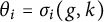 $\theta _i=\sigma _i(g,k)$
with
 $i\geqslant 1$
is the ith element of the sequence of eigenvalues
 $\{\sigma _i(g,k)\}$
arranged in increasing order, when we fix the Laplacian eigenvalue
 $\lambda =k$
in (1.1) (we call these eigenvalues the Steklov eigenvalues of frequency k). Also
 $\omega _i=\sigma _i(g,-k)$
, the Steklov eigenvalues of frequency
 $-k$
, are defined by setting
 $\lambda =-k$
. They will be our first class of candidates that characterize metrics admitting the desired FBMI or FBHM. These functionals
 $\Theta _{r,i}$
and
 $\Omega _{r,i}$
have the exact same form as in the two-dimensional case (see [Reference Lima and Menezes26, Reference Medvedev28]), but are defined for a compact k-dimensional manifold with boundary. A reasoning of why the functionals are in such forms is given in Section 2.2. The motivation for these functionals is provided by Theorems 1.1, 1.2, 3.1, and 3.2 below: their extremal metrics correspond to those induced by FBMI and FBHM – depending on the domain – of a compact k-dimensional manifold with boundary in geodesic balls in
 $\mathbb {S}^m_+$
(in the case of
 $\Theta _{r,i}$
) and in
 $\mathbb {H}^m$
(in the case of
 $\Omega _{r,i}$
).
We also introduce the following functionals defined on the set
 $\mathcal {R}(\Sigma ^k)$
using Laplacian eigenvalues:
 $$ \begin{align*}\Xi_{r,i}^+(\Sigma,g):=\min\left\lbrace \lambda_0(g,-\tan(r)), \lambda_i(g, \cot(r))\right\rbrace|\Sigma|_g^{2/k},\ i\geqslant 1, \, 0<r<\frac{\pi}{2} \end{align*} $$
and
 $$ \begin{align*}\Xi_{r,i}^-(\Sigma,g):=\min\{\lambda_0(g, \tanh(r)),\lambda_i(g, \coth(r))\}|\Sigma|_g^{2/k},\, i\geqslant 1, \, r>0. \end{align*} $$
Here,
 $\lambda _i(g,\cdot )$
is the ith component of the increasing sequence of Laplacian eigenvalues. We will demonstrate the relationship between the critical points of these functionals and metrics admitting FBMI or FBHM into geodesic balls in
 $\mathbb {S}^m_+$
or
 $\mathbb {H}^m$
, summarized in the following theorems.
Theorem 1.1 Let
 $\Sigma ^k$
be a k-dimensional compact smooth manifold with boundary. For
 $r<\dfrac {\pi }{2}$
and
 $i\geqslant 1$
, let
 $\mathbb B^m(r)$
denote a ball of radius r in
 $\mathbb {S}^m$
centered at the point
 $(1,0,\ldots ,0)$
and
 $V_i(g)$
be the eigenspace of the Steklov eigenvalue
 $\theta _i$
with frequency k. Then, the following are true:
-
• If g is an extremal metric for
 $\Theta _{r,i}$
on the class
$\mathcal {R}_{k}(\Sigma )$
, then there exist
$v_0\in V_0(g)$
and
$v_1,\ldots ,v_m\in V_i(g)$
such that the following map is in fact an FBMI into
$$ \begin{align*}\Phi:\Sigma\rightarrow \mathbb{R}^{m+1},\ x\mapsto (v_0(x),v_1(x),\ldots,v_m(x))\end{align*} $$
$\mathbb B^m(r)$
.
-
• If g is an extremal metric for
$\Theta _{r,i}$
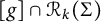
on a Riemannian conformal class
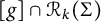
$[g]\cap \mathcal {R}_{k}(\Sigma )$
, then there exist
$v_0\in V_0(g)$
and
$v_1,\ldots ,v_m\in V_i(g)$
such that the map
$\Phi $
is an FBHM into
$\mathbb B^m(r)$
.










Theorem 1.2 Given
 $i\geqslant 1$
, suppose that for some
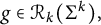 $g\in \mathcal {R}_{k}(\Sigma ^k),$
we have either
 $\theta _i(g)<\theta _{i+1}(g)$
or
 $\theta _i(g)>\theta _{i-1}(g)$
. Let
 $V_i(g)$
be the eigenspace of the Steklov eigenvalue
 $\theta _i$
of frequency k:
-
• Suppose there exist
$v_0\in V_0(g)$
and independent
$v_1,\ldots ,v_m\in V_i(g)$
such that:-
(1)
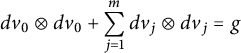
$dv_0\otimes dv_0+\displaystyle \sum _{j=1}^m dv_j\otimes dv_j=g$
; -
(2)
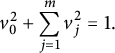
$v_0^2+\displaystyle \sum _{j=1}^m v_j^2=1.$
Then, there is some
$0<r<\dfrac {\pi }{2}$
such that g is an extremal metric for
$\Theta _{r,i}$
in the set
$\mathcal {R}_{k}(\Sigma )$
. -
-
• If there exist
$v_0\in V_0(g)$
and independent
$v_1,\ldots ,v_m\in V_i(g)$
such that
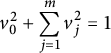
$v_0^2+\displaystyle \sum _{j=1}^m v_j^2=1$
, the metric g is extremal for
$\Theta _{r,i}$
in the set
$[g]\cap \mathcal {R}_{k}(\Sigma )$
for some
$0<r<\dfrac {\pi }{2}$
.







In these two theorems,
 $\mathcal {R}_{k}(\Sigma )$
denotes the subset of Riemannian metrics on
 $\Sigma $
, which do not admit k as a Dirichlet eigenvalue. This restriction is necessary (see Section 2) in the spherical case.
In Section 3, we also prove similar theorems for FBMI and FBHM into a geodesic ball in
 $\mathbb H^m$
.
It turns out that the metrics induced by FBMI into geodesic balls in the hemisphere can be obtained in a different approach. Namely, instead of the functional
 $\Theta _{r,i}$
on
 $\mathcal R_{k}(\Sigma ^k)$
, one can take the functional
 $\Xi _{r,i}^+(\Sigma ,g)$
, defined above, on the set of all metrics on
 $\Sigma $
. This functional admits extremal metrics, which are metrics induced by FBMI into geodesic balls in the unit hemisphere. The formal statement is as follows.
Theorem 1.3 The functional
 $\Xi _{r,i}^-(\Sigma ,g)$
has no extremal metrics on
 $\mathcal {R}(\Sigma )$
, and the functional
 $\Xi _{r,i}^+(\Sigma ,g)$
has extremal metrics on
 $\mathcal {R}(\Sigma )$
only if
 $$ \begin{align} \lambda_0(g,- \tan(r))=\lambda_i(g, \cot(r)). \end{align} $$
Moreover, if g is an extremal metric for
 $\Xi _{r,i}^+(\Sigma ,g)$
, then there exist
 $v_0\in E_0(g,-\tan r)$
and
 $v_1,\ldots ,v_m\in E_i(g,\cot r)$
such that the map
 $(v_0,v_1,\ldots ,v_m)$
induces an FBMI from
 $\Sigma $
into the geodesic ball
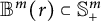 $\mathbb B^m(r)\subset \mathbb {S}^m_+$
centered at
 $(1,0,\ldots ,0)$
.
Here,
 $E_i(g,\sigma )$
is the ith eigenspace of problem 1.1 with
 $\sigma $
given. Theorem 1.3 actually states that it is senseless to consider the functional
 $\Xi _{r,i}^-(\Sigma ,g)$
from the point of view of extremal metrics. However, considering the functional
 $\Xi _{r,i}^+(\Sigma ,g)$
is meaningful. Particularly, one can be interested in finding maximal and minimal metrics for
 $\Xi _{r,i}^+(\Sigma ,g)$
. This leads us to the question of whether this functional is bounded. In Proposition 4.1, we show that both functionals
 $\Xi _{r,i}^+(\Sigma ,g)$
and
 $\Xi _{r,i}^-(\Sigma ,g)$
are bounded from above on the set of Riemannian metrics for any compact surface with boundary. For
 $\Xi _{r,1}^+(\Sigma ,g)$
, we were also able to find an explicit upper bound in the following theorem, which was inspired by Theorem A in [Reference Lima and Menezes26].
Theorem 1.4 For any compact surface
 $\Sigma $
with boundary, one has
 $$ \begin{align*}\Xi_{r,1}^+(\Sigma,g)\leqslant 4\pi(1-\cos r)(\gamma+l), \end{align*} $$
where
 $\gamma $
and l are, respectively, the genus and the number of boundary components. If
 $\Sigma $
is a topological disk, then
 $$ \begin{align*}\Xi_{r,1}^+(\Sigma,g)\leqslant 4\pi(1-\cos r), \end{align*} $$
and the equality holds if and only if
 $\Sigma $
is a geodesic disk in
 $\mathbb B^2(r)\subset \mathbb S^2_+$
.
However, in Proposition 4.2, we show that both functionals are not bounded from below even in any conformal class. These results imply that one can find maximal metrics for
 $\Xi _{r,i}^+(\Sigma ,g)$
on
 $\mathcal R(\Sigma )$
, but there are no minimal metrics for it on
 $\mathcal R(\Sigma )$
. Moreover, the canonical metric on a geodesic disk in
 $\mathbb B^2(r)\subset \mathbb S^2_+$
is maximal for
 $\Xi _{r,1}^+(\Sigma ,g)$
when
 $\Sigma $
is a topological disk. We conjecture that the metric on the critical spherical catenoid in a geodesic ball in
 $\mathbb S^3_+$
(see [Reference Do Carmo and Dajczer5]) is maximal for
 $\Xi _{r,1}^+(\Sigma ,g)$
on the topological annulus. There is also a candidate for a maximal metric for
 $\Xi _{r,1}^+(\Sigma ,g)$
on the topological Möbius band. It would be interesting to find other maximal metrics.
In conclusion, we would like to emphasize that the main advantage of the functional
 $\Xi _{r,i}^+$
with respect to
 $\Theta _{r,i}$
is that we do not restrict the set of all Riemannian metrics on
 $\Sigma $
to the set of admissible metrics. Particularly, in Theorem 1.4, we find a maximal metric for a topological disk on the set of all Riemannian metrics.
1.1 Article organization
This article is organized as follows. Section 2 is dedicated to FBMI in geodesic balls in
 $\mathbb S^n_+$
. More precisely, in Section 2.1, we prove Theorem 1.1. Here, we also show Theorem 1.2. In Section 2.2, we give a justification for why the functional
 $\Theta _{r,i}$
is in the same form as the two-dimensional case given by [Reference Lima and Menezes26]. In Section 3, we prove similar theorems for the case of FBMI in geodesic balls in
 $\mathbb H^n$
. In Section 4, we treat the functionals
 $\Xi ^\pm _{r,i}$
. Here, we prove Theorems 1.3 and 1.4.
2 FBMI in spheres
2.1 Critical metrics of sphere FBMI functional
We follow the notation conventions in [Reference Lima and Menezes26, Reference Medvedev28]. Let
 $\Sigma ^k$
be a k-dimensional compact manifold with (sufficiently smooth, e.g., Lipschitz) boundary. Recall that
 $\mathcal {R}_{k}(\Sigma )$
denotes the subset of Riemannian metrics on
 $\Sigma $
such that the following PDE system has no nonzero solutions:
 $$ \begin{align*} \left\{ \begin{aligned} & -ku+ \Delta_g u =0\ &\mathrm{in}\ \Sigma,\\ & u =0\ &\mathrm{on}\ \partial\Sigma. \end{aligned} \right. \end{align*} $$
In other words,
 $\mathcal {R}_{k}(\Sigma )$
denotes the set of metrics on
 $\Sigma $
, for which k is not a Dirichlet eigenvalue. For
 $g\in \mathcal {R}_{k}(\Sigma )$
, we consider the following linear PDE system with parameter
 $\theta :$
 $$ \begin{align} \left\{ \begin{aligned} -ku+\Delta_g u=0\ &\mathrm{in}\ \Sigma,\\ \dfrac{\partial u}{\partial \eta}=\theta u\ &\mathrm{on}\ \partial\Sigma, \end{aligned} \right. \end{align} $$
where
 $\eta $
in the unit outer normal to
 $\partial \Sigma $
in
 $(\Sigma ,g)$
. The Steklov eigenvalues of g with frequency k are real numbers
 $\theta $
, for which the above system has nontrivial solutions. Arrange these eigenvalues in increasing order, counted with multiplicity, by
 $\theta _i$
for
 $i\geqslant 0$
. Let
 $V_i(g)$
be the space of eigenfunctions corresponding to
 $\theta _i$
. It is known that
 $( \theta _i)_{i\in \mathbb N}$
is discrete with
 $\theta _i\rightarrow +\infty $
, as
 $i\to \infty $
and
 $\theta _0$
is simple, when
 $\Sigma $
is connected.
For any
 $0<r<\dfrac {\pi }{2}$
and
 $i\geqslant 1$
, let
 $\Theta _{r,i}$
be the following functional on
 $\mathcal {R}_{k}(\Sigma )$
as in [Reference Medvedev28]:
 $$ \begin{align} \Theta_{r,i}(\Sigma,g) := (\theta_0(g)\cos^2 r+\theta_i(g)\sin^2 r)\vert\partial \Sigma\vert_g + 2\vert \Sigma\vert_g. \end{align} $$
This is exactly the same functional as in [Reference Lima and Menezes26], for which the critical metrics induce FBMI into unit spherical caps by Laplace eigenfunctions when
 $k=2$
. We will see that this functional also serves the same purpose when
 $k>2$
.
The first problem arising in finding extremal metrics of this functional is that the eigenvalues
 $\theta _i(g_t)$
can be non-differentiable even for a smooth family of metrics
 $(g_t)_{t\in [-\varepsilon ,\varepsilon ]}$
. Fix any
 $\varepsilon>0$
and let
 $(g_t)_{ [-\varepsilon ,\varepsilon ]}\in \mathcal {R}_{k}(\Sigma )$
be a smooth family of admissible metrics on
 $\Sigma $
. Then, each function
 $t\mapsto \theta _i(g_t)$
is Lipschitz in t (see, e.g., [Reference Medvedev28, Claim 4]). Thus, the functional
 $\Theta _{r,i}(g(t))$
is differentiable almost everywhere. We compute an explicit form of the derivative of
 $\Theta _{r,i}(g_t)$
, which is well-defined for almost every t, following the approach in [Reference Lima and Menezes26]. Let
 $g^b_t$
be the restriction of
 $g_t$
to
 $\partial \Sigma $
, and denote
 $dA_t$
and
 $dL_t$
the volume density, induced by
 $g_t$
and
 $g^b_t$
on
 $\Sigma $
and
 $\partial \Sigma $
, respectively. When
 $\theta _i(g_t)$
is differentiable, its derivative is given by
 $$ \begin{align*} \dfrac{d}{dt}\left(\theta_i(g_t) \right)= & \int_{\Sigma} \left\langle \dfrac{1}{2}\left(-k u_i^2(t)+ \vert \nabla^t u_i(t) \vert_{g_t}^2 \right)g_t- du_i(t)\otimes du_i(t), \dot{g}(t) \right\rangle_{g_t} dA_t\\ & -\theta_i(g_t)\int_{\partial \Sigma} \dfrac{1}{2} u_i^2(t) \left\langle g^b_t,\dot{g}^b_t \right\rangle_t dL_t, \end{align*} $$
where
 $u_i(t)$
is some eigenfunction of
 $\theta _i(g_t)$
such that
 $\Vert u_i(t)\Vert _{L^2(\partial \Sigma , dL_t)}=1$
. Therefore, the weak derivative of
 $\Theta _{r,i}(g_t)$
is given by
 $$ \begin{align} \begin{aligned} Q_r(u_0(t),u_i(t)) &:= \dfrac{d}{dt}\left( \Theta_{r,i}(g_t) \right)\\ &= \int_{\Sigma} \left\langle \tau^k_t(\cos r \cdot u_0(t))+\tau^k_t(\sin r \cdot u_i(t))+ g,\dot{g}_t \right\rangle_t dA_t \\ &\quad +\int_{\partial\Sigma} F^k_t(\cos r \cdot u_0(t),\sin r\cdot u_i(t))\left\langle g^b, \dot{g}^b \right\rangle_t dL_t. \end{aligned} \end{align} $$
Here, the functions
 $\tau ^k_t$
and
 $F^k$
are defined analogously as in [Reference Lima and Menezes26] by
 $$ \begin{align*} \tau^k(u) &=\vert \partial\Sigma_t\vert\left( \dfrac{1}{2}\left(-ku^2+\vert \nabla^t u\vert_{g_t}^2\right)g-du\otimes du \right),\\ F^k(v_1,v_2) &=\dfrac{1}{2} \bigg( \theta_0\left(\cos^2 r -\vert \partial\Sigma_{g_t}\vert v_1^2 \right)+ \theta_i\left(\sin^2 r -\vert \partial\Sigma_{g_t}\vert v_2^2 \right)\bigg ). \end{align*} $$
We want to recall several facts from [Reference Lima and Menezes26]. The weak derivative
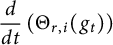 $\dfrac {d}{dt}\left ( \Theta _{r,i}(g_t) \right )$
given by (2.3) is a sum of two integrals. We call the integral on
 $\Sigma $
the interior component and the integral on
 $\partial \Sigma $
the boundary component. We can rewrite the formula (2.3) as the following inner product on the space
 $L^2(S^2(\Sigma ,g))\times L^2(\partial \Sigma ,g^b):$
 $$ \begin{align*} \bigg\langle & \left(\dot{g}_t,\langle g^b,\dot{g}^b \rangle_t \right) , \\ & \left( \tau^k_t(\cos r \cdot u_0(t))+\tau^k_t(\sin r \cdot u_i(t))+ g, F^k_t(\cos r \cdot u_0(t),\sin r\cdot u_i(t)) \right) \bigg\rangle; \end{align*} $$
see [Reference Lima and Menezes26, Section 5] for details. Also, note that
 $\theta _0(t)$
is a simple eigenvalue for connected
 $\Sigma ^k$
, so we can assume that
 $u_0(t)$
has a unique choice for each t. Thus, for a fixed smooth family of metrics
 $(g_t)_{t\in [-\varepsilon ,\varepsilon ]}$
, for each given t, the above inner product is actually a function of
 $u_i^2(t)$
.
Although
 $\Theta _{r,i}(g_t)$
is not always differentiable, for a smooth family of metrics
 $(g_t)_{t\in [-\varepsilon ,\varepsilon ]}$
, the functional
 $Q_r(u_0(t),u_i(t))$
given by (2.3) is always defined. Now, suppose g is an extremal metric for
 $\Theta _{r,i}$
. Let
 $(g_t)_{t\in [-\varepsilon ,\varepsilon ]}$
be a smooth family such that
 $\Theta _{r,i}(g_t)\leqslant \Theta _{r,i}(g)+o(t)$
with
 $g_0=g$
. Since
 $\Theta _{r,i}(g_t)$
is absolute continuous, by the Lebesgue fundamental theorem of calculus, we see that there exist
 $t_j^+\rightarrow 0^+$
and
 $t_j^-\rightarrow 0^-$
such that the
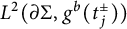 $L^2(\partial \Sigma ,g^b(t_j^{\pm }))$
-normalized eigenfunctions
 $u_i(t_j^{\pm })$
of
 $\theta _i(t_j^{\pm })$
satisfy
 $$ \begin{align*} \limsup_{j\rightarrow\infty} Q_r(u_0(t_j^+),u_i(t_j^+))\leqslant 0,\ \liminf_{j\rightarrow\infty} Q_r(u_0(t_j^-),u_i(t_j^-))\geqslant 0. \end{align*} $$
An analogous statement also holds for the case
 $\Theta _{r,i}(g_t)\geqslant \Theta _{r,i}(g)+o(t)$
. Therefore, we can argue as in [Reference Lima and Menezes26, Lemma 3] to prove exactly the same statement as follows.
Lemma 2.1 Suppose g is an extremal metric of
 $\Theta _{r,i}$
. For any
 $(h,\psi )\in L^2(S^2(\Sigma ,g))\times L^2(\partial \Sigma ,g^b)$
, there exists
 $u_i$
, which is an eigenfunction corresponding to
 $\theta _i$
with
 $\Vert u_i \Vert _{L^2(\partial \Sigma ,g^b)} =1$
such that
 $$ \begin{align*} \Big\langle\!\! \left( h,\psi \right) , \left( \tau^k_t(\cos r \cdot u_0(t))+\tau^k_t(\sin r \cdot u_i(t))+ g, F^k_t(\cos r \cdot u_0(t),\sin r\cdot u_i(t)) \right) \!\!\Big\rangle\! =0. \end{align*} $$
Now, we can prove Theorem 1.1, which extends the results by Lima and Menezes in [Reference Lima and Menezes26] and the second author in [Reference Medvedev28] to the higher-dimensional case.
Proof of Theorem 1.1
We begin by proving the first statement of the theorem. For fixed
 $l\geqslant 1$
, denote
 $V_l(g)$
the eigenspace corresponding to the eigenvalue
 $\theta _l$
for
 $g\in \mathcal {R}_{k}(\Sigma )$
and
 $l=0\ \mathrm {or} \ i$
. For any
 $g\in \mathcal {R}_{k}(\Sigma )$
, we define the following subset of
 $ L^2(S^2(\Sigma ),g)\times L^2(\partial \Sigma ,g^b):$
 $$ \begin{align*} \mathcal{C}_r:=\Big\lbrace & \left(\tau^k (\cos r\cdot u_0)+\tau^k(\sin r\cdot u_i)+ g,\ F^k(\cos r \cdot u_0,\sin r \cdot u_i) \right): \\ & u_0\in V_0(g),\ u_i\in V_i(g),\ \Vert u_0\Vert_{L^2(\partial\Sigma,g^b)}=\Vert u_i\Vert_{L^2(\partial\Sigma,g^b)}=1 \Big\rbrace. \end{align*} $$
This subset is actually obtained by the formula of the weak derivative of
 $\Theta _{r,i}(g_t)$
with
 $g(0)=g$
. If
 $g\in \mathcal {R}_{k}(\Sigma )$
is a critical point of the functional
 $\Theta _{r,i}$
, the point
 $(0,0) $
is in the convex hull of the set
 $\mathcal {C}_r(g)$
by the geometric Hahn–Banach theorem (see [Reference Lima and Menezes26, p. 17]). For simplicity, denote
 $a=|\partial \Sigma |_g$
. We can find
 $L^2(\partial \Sigma ,g^b) $
-normalized functions
 $u_0\in V_0(g)$
and
 $u_1,\ldots ,u_m\in V_i(g)$
together with constants
 $t_j>0$
and
 $\displaystyle \sum _{j=1}^m t_j=1$
such that
 $$ \begin{align} \displaystyle \sum_{j=1}^m t_j \left[ \theta_0 \cos^2 r \left( 1- au_0^2 \right) +\theta_i \sin^2 r \left(1-a u_j^2 \right) \right]=0\ \mathrm{on}\ \partial \Sigma. \end{align} $$
Denote the rescaled functions by
 $$ \begin{align} v_0= \sqrt{a}\cos r \cdot u_0,\ v_j= \sqrt{a t_j}\sin r \cdot u_j,\ \mathrm{for}\ 1\leqslant j\leqslant m, \end{align} $$
and define
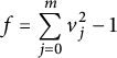 $f=\displaystyle \sum _{j=0}^m v_j^2-1$
. Notice that a priori f is not identically zero on
 $\partial \Sigma $
. However, it is easy to verify that
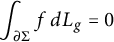 $\displaystyle \int _{\partial \Sigma }f\,dL_g=0$
. Now, let
 $\eta $
be the outward-pointing unit normal vector field on
 $\partial \Sigma $
, we have from (2.4) that
 $$ \begin{align} \dfrac{\partial f}{\partial \eta}=2(\theta_0\cos^2 r+\theta_i \sin^2 r) \end{align} $$
is a constant.
The interior component of the weak derivative gives
 $$ \begin{align} g+\dfrac{1}{2}\sum_{j=0}^m \left(-k v_j^2+\vert \nabla^g v_j\vert^2 \right) g-\sum_{j=0}^m dv_j\otimes dv_j=0. \end{align} $$
Raising the indices using
 $g^{-1}$
, and taking the trace of the above equation yields
 $$ \begin{align} k+\left(\dfrac{k}{2}\sum_{j=0}^m\vert \nabla^g v_j\vert^2-\dfrac{k^2}{2}\sum_{j=0}^m v_j^2-\sum_{j=0}^m \vert\nabla^g v_j\vert^2 \right)=0. \end{align} $$
Using equation (2.8), we get
 $$ \begin{align*} \Delta_g f=\dfrac{-4k}{k-2}f. \end{align*} $$
Note that
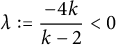 $\lambda :=\dfrac {-4k}{k-2}<0$
for all
 $k>2$
. Then, using the divergence theorem, we get
 $$ \begin{align*} 0 \leqslant -\lambda \int_{\Sigma}f^2\,dA_g+ \int_{\Sigma}\vert \nabla^g f\vert_g^2 dA_g&=\int_{\Sigma} (-\Delta_g f\cdot f + \vert \nabla^g f\vert_g^2 )dA_g\\& = \int_{\partial\Sigma} f\cdot \dfrac{\partial f}{\partial \eta}dL_g= \dfrac{\partial f}{\partial \eta}\int_{\partial\Sigma} f dL_g=0. \end{align*} $$
This is only possible, when
 $f\equiv 0$
on
 $\Sigma $
, i.e.,
 $\displaystyle \sum _{j=0}^m v_j^2=1$
on
 $\Sigma $
. Substituting this back to (2.7) and (2.8), we see that one has
 $$ \begin{align*}\sum_{j=0}^m \vert\nabla^g v_j\vert^2=k \quad \text{and} \quad g=\sum_{j=0}^m dv_j\otimes dv_j. \end{align*} $$
Therefore, the map
 $$ \begin{align*} \Phi:\Sigma\rightarrow \mathbb{R}^{m+1},\ \Phi(x)=(v_0(x),v_1(x),\ldots,v_m(x)) \end{align*} $$
is an isometric immersion into
 $\mathbb {S}^m$
. Since
 $\dfrac {\partial f}{\partial \eta }=0$
on
 $\partial \Sigma $
, it follows trivially from the steps of the proof of Theorem B in [Reference Lima and Menezes26], that
 $v_0=\cos r$
on
 $\partial \Sigma $
,
 $\theta _0=-\tan r,$
and
 $\theta _i=\cot r$
. This implies that
 $\Phi $
is an FBMI of
 $\Sigma $
into
 $\mathbb B^m(r)$
.
Now, we examine the extremal metrics for the functional
 $\Theta _{r,i}$
on the set of conformal admissible metrics for a given
 $i\geqslant 1$
as before. Let
 $g\in \mathcal R_{k}(\Sigma )$
be a Riemannian metric such that
 $\Theta _{r,i}(g)$
is extremal for the conformal class
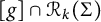 $[g]\cap \mathcal R_{k}(\Sigma )$
. We claim that similarly to the two-dimensional case in [Reference Lima and Menezes26, Reference Medvedev28], there exist frequency k Steklov eigenfunctions inducing an FBHM into
 $\mathbb B^m(r)$
.
Since g is extremal for
 $\Theta _{r,i}$
, the weak derivative of
 $\Theta _{r,i}$
vanishes at g when restricting to the conformal class
 $[g]$
. We obtain the following result similar to Lemma 2.1: for any positive functions
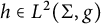 $h\in L^2(\Sigma ,g)$
and
 $h_b\in L^2(\partial \Sigma ,g^b),$
we can find
 $L^2(\partial \Sigma ,g^b)$
-normalized functions
 $u_0\in V_0(g)$
and
 $u_i\in V_i(g)$
such that
 $$ \begin{align} \int_{\partial\Sigma} h_b \left(\theta_0 \cos^2r \left(1-a u_0^2\right) +\theta_i \sin^2 r \left(1-a u_i^2\right) \right)dL_g=0 \end{align} $$
and also
 $$ \begin{align} &{{\int_{\Sigma}}} h \left( a \left( \cos^2 r \left(-\dfrac{k^2}{2}u_0^2+\left(\dfrac{k}{2}-1\right)\vert \nabla^g u_0\vert^2 \right) \right. \right. \nonumber\\ &\quad \left.\left. + \sin^2 r \left( -\dfrac{k^2}{2}u_i^2+\left(\dfrac{k}{2}-1\right)\vert \nabla^g u_i\vert^2 \right) \right) +k \right)dA_g=0. \end{align} $$
Therefore, similarly to the proof of FBMI case for critical metrics on the whole admissible class above, equation (2.9) and the geometric Hahn–Banach theorem imply that there exist
 $L^2(\partial \Sigma ,g^b)$
-normalized eigenfunctions
 $u_0\in V_0(g)$
and
 $u_j\in V_i(g)$
for
 $1\leqslant j\leqslant m $
together with
 $t_j>0$
with
 $\sum _j t_j=1$
such that (2.4) holds. Rescale these eigenfunctions as in (2.5) to obtain
 $v_0,v_1,\ldots ,v_m$
. For
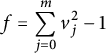 $f=\displaystyle \sum _{j=0}^m v_j^2-1$
, we also obtain (2.6) as in the general case. Moreover, the trick used for (2.9) applied to equation (2.10) shows that (2.8) also holds. Therefore, we can also deduce that
 $\displaystyle \sum _{j=0}^m v_j^2=1$
. We see that map
 $\Phi : \Sigma \rightarrow \mathbb {R}^{m+1}$
defined by
 $x\mapsto (v_0(x),v_1(x),\ldots ,v_m(x))$
has image inside
 $\mathbb {S}^m$
. Finally, combining equations (2.4) and
 $\dfrac {\partial f}{\partial \eta }=0$
on
 $\partial \Sigma $
together, we have
 $v_0=\cos r$
on
 $\partial \Sigma $
, see also proof of Theorem B in [Reference Lima and Menezes26].
We now prove Theorem 1.2, which serves as a converse to Theorem 1.1 under the following additional assumption.
For some fixed integer
 $i \geqslant 1$
and a given Riemannian metric g, either
 $\theta _i < \theta _{i+1}$
or
 $\theta _i> \theta _{i-1}$
.
This assumption ensures that, for any smooth variation
 $g_t$
of the metric with
 $g_0 = g$
, the eigenvalue branch
 $\theta _i(g_t)$
is extremal – specifically, it is the largest (respectively, smallest) among all eigenvalues
 $\{\theta _l(g_t)\}$
satisfying
 $\theta _l(g_0) = \theta _i(g_0)$
– for t sufficiently close to
 $0$
, provided that
 $\theta _i < \theta _{i+1}$
(respectively,
 $\theta _i> \theta _{i-1}$
).
To understand this condition, recall that when the eigenvalue
 $\theta _i(g_0)$
has multiplicity greater than one, the function
 $t \mapsto \theta _i(g_t)$
is generally not differentiable at
 $t = 0$
. Instead, it admits distinct one-sided derivatives, corresponding to different choices of
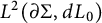 $L^2(\partial \Sigma , dL_0)$
-normalized eigenfunctions
 $u_j \in V_i(g)$
inserted into the expression (2.3). However, the extremality (maximality in the case
 $\theta _i < \theta _{i+1}$
and minimality in the case
 $\theta _i> \theta _{i-1}$
) of
 $\theta _i(g_t)$
near
 $t = 0$
allows us to compare the relevant one-sided derivatives with the value obtained by substituting a specific
 $L^2(\partial \Sigma , dL)$
-normalized eigenfunction
 $u_j \in V_i(g)$
into (2.3).
Proof of Theorem 1.2
We prove the first statement following the steps in [Reference Medvedev28, Proposition 3.3] as the second statement is totally analogous. Applying the normal derivative
 $\partial \eta $
to the equation
 $$ \begin{align*}\displaystyle\sum_{j=0}^m v_j^2=1,\end{align*} $$
we obtain
 $$ \begin{align*} \theta_0 v_0^2+\theta_i(1-v_0^2)=0\ \mathrm{on}\ \partial\Sigma. \end{align*} $$
Since
 $\theta _i-\theta _0>0$
, we see that
 $v_0^2$
is a constant on
 $\partial \Sigma $
. If we have
 $v_0^2=0$
on
 $\partial \Sigma $
, the equation above implies that
 $\theta _i=0$
. In addition, the fact that
 $g\in \mathcal {R}_{k}(\Sigma )$
gives
 $v_0\equiv 0$
on
 $\Sigma $
and
 $\theta _0=0$
. This leads to a contradiction. Similarly, we obtain that
 $\displaystyle \sum _{j=1}^m v_j^2$
is a nonzero constant on
 $\partial \Sigma $
. Therefore, there is some
 $0<r<\dfrac {\pi }{2}$
such that
 $$ \begin{align*} v_0^2=\cos^2 r,\ \sum_{j=1}^m v_j^2=\sin^2 r\ \mathrm{on}\ \partial\Sigma. \end{align*} $$
Now rescale these functions, we obtain
 $L^2(\partial \Sigma ,g^b)$
-normalized eigenfunctions
 $u_0,u_1,\ldots ,u_m$
, and set the constants
 $$ \begin{align*} t_j=\dfrac{1}{a\sin^2 r}\Vert v_j\Vert^2_{L^2(\partial\Sigma,g^b)},\ \forall 1\leqslant j\leqslant m. \end{align*} $$
We see that
 $t_j>0$
and
 $\displaystyle \sum _{j=1}^m t_j=1$
. Analogously to [Reference Medvedev28, Proposition 3.3], we have
 $$ \begin{align} \sum_{j=1}^m t_j Q_r(u_0,u_j)=0. \end{align} $$
Thus, in the summation above, there exist terms
 $Q_r(u_0, u_j)$
nonnegative and nonpositive. Note that
 $\theta _0(g_t)$
is always simple. Let us fix an index
 $i \geqslant 1$
and consider the set of indices
 $$ \begin{align*}I_i := \bigl\{ l \in \mathbb{N} \,\big|\, \theta_l(g_0) = \theta_i(g_0) \bigr\}, \end{align*} $$
i.e., all eigenvalues that coincide with
 $\theta _i(g_0)$
at
 $t = 0$
. We now invoke the key assumption from Theorem 1.2: either
 $\theta _i(g_0) < \theta _{i+1}(g_0)$
or
 $\theta _i(g_0)> \theta _{i-1}(g_0)$
. Under this hypothesis, for any smooth variation
 $g_t$
with
 $g_0 = g$
, the branch
 $\theta _i(g_t)$
is extremal among
 $\{\theta _l(g_t)\}_{l \in I_i}$
for
 $|t|$
sufficiently small – specifically, it is the largest such eigenvalue if
 $\theta _i(g_0) < \theta _{i+1}(g_0)$
, and the smallest if
 $\theta _i(g_0)> \theta _{i-1}(g_0)$
.
Assume first that
 $\theta _i(g_t)$
is the smallest eigenvalue among
 $\{\theta _l(g_t)\}_{l \in I_i}$
for t near
 $0$
. Since
 $\sin ^2 r> 0$
, the variational characterization implies that there exists a normalized eigenfunction
 $u_j^+ \in V_i(g)$
such that
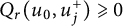 $Q_r(u_0, u_j^+) \geqslant 0$
. The minimality of
 $\theta _i(g_t)$
ensures that the left derivative of
 $\Theta _{r,i}(g_t)$
at
 $t = 0$
is bounded below by this value:
 $$ \begin{align*}\lim_{t \to 0^-} \frac{\Theta_{r,i}(g_t) - \Theta_{r,i}(g_0)}{t} \geqslant Q_r(u_0, u_j^+) \geqslant 0. \end{align*} $$
Similarly, there exists another normalized eigenfunction
 $u_j^- \in V_i(g)$
with
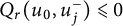 $Q_r(u_0, u_j^-) \leqslant 0$
, and the minimality again guarantees that the right derivative satisfies
 $$ \begin{align*}\lim_{t \to 0^+} \frac{\Theta_{r,i}(g_t) - \Theta_{r,i}(g_0)}{t} \leqslant Q_r(u_0, u_j^-) \leqslant 0. \end{align*} $$
These inequalities imply that the one-sided derivatives of
 $\Theta _{r,i}(g_t)$
at
 $t = 0$
do not have the same definite sign; hence, g is an extremal metric for the functional
 $\Theta _{r,i}$
.
An entirely analogous argument applies when
 $\theta _i(g_t)$
is the largest eigenvalue among
 $\{\theta _l(g_t)\}_{l \in I_i}$
(which occurs under the alternative assumption
 $\theta _i(g_0) < \theta _{i-1}(g_0)$
). In that case, the roles of the upper and lower bounds are reversed, but the conclusion remains the same. Thus, g is again extremal for
 $\Theta _{r,i}$
.
This completes the proof.
2.2 Coefficients of the sphere FBMI functional
We provide a justification why the functional defined in (2.2) is of the same form as the functional in [Reference Lima and Menezes26] for the two-dimensional case. One natural question is whether there are functionals in a similar form that give rise to critical metrics induced by FBMI in a geodesic ball in the standard sphere. We consider the functionals in the following form:
 $$ \begin{align} \Theta_r(\Sigma,g)=(\cos^2 r\theta_0+\sin^2 r\theta_1)\alpha_1 a^{\beta_1}+\alpha_2 A^{\beta_2}. \end{align} $$
Here,
 $a=\vert \partial \Sigma \vert _g$
and
 $A=\vert \Sigma \vert _g$
for simplicity, and
 $\alpha _1,\alpha _2,\beta _1$
, and
 $\beta _2$
are given constants. Note that if we set
 $i=1$
, then (2.2) belongs to the class of functionals given by (2.12). We would like to investigate whether there are other choices of the coefficients
 $\alpha _l,\beta _l$
such that the functional in the form of (2.12) would have critical metrics, induced by FBMI in a geodesic ball in the standard sphere.
We want the critical points of (2.12) to include all the metrics whose eigenfunctions corresponding to the Steklov eigenvalues
 $\theta _0,\theta _1$
(of frequency k) induce FBMI embeddings into unit spherical caps. Let
 $\mathbb B^k(r)$
be the spherical cap in
 $\mathbb {S}^k$
at
 $(1,0,\ldots ,0)$
. The coordinate functions are spherical harmonics of degree
 $1$
. Therefore,
 $\Delta _g x_i-k x_i=0$
, for all
 $i=0,\ldots ,k$
. Regarding the Steklov eigenvalues and eigenfunctions, Theorem 3 of [Reference Lima and Menezes26] and its proof for two-dimensional spherical caps can be generalized to higher dimensions, and the detailed steps are given by the second author in the proof of Proposition 5.6 of [Reference Medvedev28]. We collect the results and obtain the following.
Proposition 2.2 For the spherical cap
 $\mathbb B^k(r)\subset \mathbb {S}^k$
centered at
 $(1,0,\ldots ,0)$
with
 $r<\dfrac {\pi }{2}$
, the eigenvalue
 $\theta _0=-\tan r$
has eigenfunction
 $x_0$
, and the eigenvalue
 $\theta _1=\cot r$
has eigenspace generated by
 $x_1,\ldots ,x_k$
. For a geodesic ball
 $\mathbb {B}^k(r)\subset \mathbb {H}^k$
centered at
 $(1,0,\ldots ,0)$
, the eigenvalue
 $\omega _0=\tanh (r)$
has eigenspace generated by
 $x_0$
, and
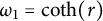 $\omega _1=\coth (r)$
has eigenspace generated by
 $x_1,\ldots ,x_k$
.
Now, we check what specific values of the parameters
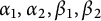 $\alpha _1,\alpha _2,\beta _1,\beta _2$
for the functionals (2.12) admit the canonical embedding of the spherical caps given in the proposition above as critical metrics. The set of extremal metric of (2.12) should include the canonical metric on
 $\mathbb B^k(r)$
. The weak derivative of
 $$ \begin{align*} \Theta_r(\mathbb{B}^k(r),g)=(\cos^2 r\theta_0+\sin^2 r\theta_1)\alpha_1 a^{\beta_1}+\alpha_2 A^{\beta_2} \end{align*} $$
is given by the following quadratic form:
 $$ \begin{align*} Q(u_0,u_1)=\alpha_1 a^{\beta_1-1}\left[ \cos^2 r(\dot{a}\beta_1\theta_0+a\dot{\theta_0})+\sin^2 r (\dot{a}\beta_1\theta_1+a\dot{\theta_1}) \right]+\alpha_2\beta_2 A^{\beta_2-1}, \end{align*} $$
where
 $u_0$
and
 $u_1$
are
 $L^2(\partial \Sigma ,g^b)$
-normalized eigenfunctions of
 $\theta _0$
and
 $\theta _1$
, respectively. They are encoded in the formulas of
 $\dot {\theta _0}$
and
 $\dot {\theta _1}$
. Thus, the boundary component of
 $Q(u_0,u_1)$
is given by
 $$ \begin{align*} Q_b=\alpha_1 a^{\beta_1-1}\cdot \dfrac{1}{2}\int_{\partial\Sigma}\left[ \theta_0\cos^2 r (\beta_1-a u_0^2)+\theta_1\sin^2 r(\beta_1-au_1^2) \right] \langle g^b,\dot{g^b}\rangle dL. \end{align*} $$
From Proposition 2.2, we see that
 $\theta _0=-\tan r$
and
 $\theta _1=\cot r$
. In addition,
 $u_0$
is a multiple of
 $x_0$
, so it is a constant on
 $\partial \Sigma $
. Suppose there are
 $L^2(\partial \Sigma ,g^b)$
-normalized eigenfunctions
 $u_0$
of
 $\theta _0$
,
 $u_1,\ldots ,u_l$
of
 $\theta _1$
and positive constants
 $\lbrace t_j\rbrace _{j=1}^l$
with
 $\displaystyle \sum _{j=1}^l t_j=1$
such that
 $$ \begin{align*} \sum_{j=1}^l Q(u_0,u_j)=0. \end{align*} $$
This gives
 $$ \begin{align*} \sum_{j=1}^l t_j u_j^2=u_0^2=\dfrac{1}{a} \equiv const,\ \partial\Sigma. \end{align*} $$
When restricting to the
 $(x_1,\ldots ,x_k)$
coordinate, we see that
 $\partial \Sigma $
is the level set of the equation
 $x_1^2+\cdots +x_k^2=\sin ^2 r$
. We know that each
 $u_j$
is a linear combination of
 $x_1,x_2,\ldots ,x_k$
. By assumption, all
 $t_j>0$
. Thus, the only possibility is
 $l=k$
and the change of coordinate from
 $(\sqrt {t_1} u_1,\ldots ,\sqrt {t_k} u_k)$
to
 $(x_1,\ldots ,x_k)$
is a linear change of basis of the form
 $cO$
, where c is a nonzero constant scaling and O is an orthogonal linear transformation. Thus, all functions
 $\sqrt {t_j}u_j$
have the same
 $L^2(\partial \Sigma ,g^b)$
-norm. Now, use the fact that each
 $u_j$
is
 $L^2(\partial \Sigma ,g^b)$
-normalized, the assumption
 $\displaystyle \sum _{j=1}^k t_j=1$
yields
 $$ \begin{align*}t_j=\dfrac{1}{k},\ \forall 1\leqslant j\leqslant k.\end{align*} $$
Using this, the substitution into the interior integral component yields
 $$ \begin{align} \alpha_1 a^{\beta_1-1}=\dfrac{1}{2}\alpha_2 \beta_2 A^{\beta_2-1}. \end{align} $$
The constants
 $\alpha _l,\beta _l$
have to depend only on k, not on a specific manifold. Therefore,
 $\dfrac {A^{\beta _2-1}}{a^{\beta _1-1}}$
has to be a fixed constant for all k-dimensional extremal metrics. This is only possible when
 $\beta _2=\beta _1=1$
. Without loss of generality, if we take
 $\alpha _1=1$
, we get
 $\alpha _2=2$
. Thus, for any k-dimensional case, the only possible functional of the form (2.12) can only be
 $$ \begin{align} \Theta_r(\mathbb{B}^k(r),g)=(\cos^2 r \theta_0+\sin^2 r \theta_1)a+2A, \end{align} $$
which is exactly the same as the two-dimensional case.
For the hyperbolic case, an analogous statement can also be proved.
Following the steps in the above spherical case, we examine the functionals in the following form:
 $$ \begin{align*} \Omega_r(\mathbb{B}^k(r),g):=(-\omega_0 \cosh^2 r+\omega_1 \sinh^2 r)\vert\partial\Sigma\vert_g^{\beta_1} +\alpha_2 \vert \Sigma\vert_g^{\beta_2}. \end{align*} $$
If we want its critical metrics to include all the canonical metrics of the geodesic balls in the hyperbolic space, then we also have
 $\beta _1=\beta _2=1$
and
 $\alpha _2=2$
.
3 FBMI in hyperbolic spaces
For the FBMI on hyperbolic spaces, we can develop results similar to the spherical case following the steps in [Reference Medvedev28]. Before introducing the theorem in the hyperbolic case, let us recall the following facts and notations.
Let
 $\Sigma ^k$
be a compact k-dimensional manifold, and
 $\mathcal {R}(\Sigma )$
be the set of all Riemannian metrics on
 $\Sigma ^k$
. Unlike the spectral problem (2.1) in the previous section, by the divergence theorem, for any metric
 $g\in \mathcal {R}(\Sigma )$
, the following PDE system has only trivial solutions:
 $$ \begin{align} \left\{ \begin{aligned} ku+ \Delta_g u =0 \ &\mathrm{in}\ \Sigma,\\ u =0\ &\mathrm{on}\ \partial\Sigma. \end{aligned} \right. \end{align} $$
For metrics
 $g\in \mathcal {R}(\Sigma )$
, the Steklov eigenvalues of frequency
 $-k$
consist of the increasing sequence of real numbers
 $\{\omega _i\}$
such that the following system has nontrivial solutions:
 $$ \begin{align} \left\{ \begin{aligned} ku+ \Delta_g u =0 \ &\mathrm{in}\ \Sigma,\\ \dfrac{\partial u}{\partial \eta} =\omega_i u\ &\mathrm{on}\ \partial\Sigma. \end{aligned} \right. \end{align} $$
For any
 $r>0$
and
 $i\geqslant 1$
, the hyperbolic FBMI functional
 $\Omega _{r,i}$
defined on
 $\mathcal {R}(\Sigma )$
in the same exact form introduced in [Reference Medvedev28] is given by the following formula, regardless the dimension k of
 $\Sigma $
:
 $$ \begin{align} \Omega_{r,i}(\Sigma,g):=(-\omega_0 \cosh^2 r+\omega_i \sinh^2 r)\vert\partial \Sigma\vert_g + 2\vert \Sigma\vert_g. \end{align} $$
Now, let
 $\tilde {\mathcal {R}}(\Sigma )$
be the subset of
 $\mathcal {R}(\Sigma )$
such that the PDE system of the following type only has zero solution:
 $$ \begin{align} \left\{ \begin{aligned} \Delta_g f-\left( \dfrac{4k}{k-2}\right)f=0 \ &\mathrm{in}\ \Sigma,\\ \dfrac{\partial f}{\partial \eta}=c \ &\mathrm{on}\ \partial\Sigma, \end{aligned} \right. \end{align} $$
where
 $c\in \mathbb {R}$
is any real constant. We prove the following theorem for the hyperbolic FBMI functionals.
Theorem 3.1 Let
 $\Sigma ^k$
with
 $k\geqslant 2$
be a k-dimensional compact smooth manifold with boundary. For
 $r>0$
, let
 $\mathbb B^m(r)$
be the ball of radius r in
 $\mathbb {H}^m$
centered at the point
 $(1,0,\ldots ,0)$
in the Minkowski space
 $\mathbb {M}^{1,m}$
, and
 $V_i(g)$
be the eigenspace of the Steklov eigenvalue
 $\omega _i$
of frequency
 $-k$
. Then, the following are true:
-
• If
$g\in \tilde {\mathcal {R}}(\Sigma )$
is an extremal metric for
$\Omega _{r,i}$
defined on
$\mathcal {R}(\Sigma )$
, then there exist
$v_0\in V_0(g)$
and
$v_1,\ldots ,v_m\in V_i(g)$
such that the following map is in fact an FBMI into
$$ \begin{align*}\Phi:\Sigma\rightarrow \mathbb{M}^{1,m},\ x\mapsto (v_0(x),v_1(x),\ldots,v_m(x))\end{align*} $$
$\mathbb B^m(r)$
.
-
• If
$g\in \tilde {\mathcal {R}}(\Sigma )$
is an extremal metric for
$\Omega _{r,i}$
on a Riemannian conformal class
$[g]$
, then there exist
$v_0\in V_0(g)$
and
$v_1,\ldots ,v_n\in V_i(g)$
such that the map
$\Phi $
is an FBHM into
$\mathbb B^m(r)$
.








Proof The case of
 $k=2$
has already been proved in [Reference Medvedev28, Proposition 3.2]. In this proof, we always assume that
 $k>2$
.
We show the first statement of theorem, following the steps in Section 2.1, and the case that restricts to the conformal class is completely analogous. Let
 $g_t\in \mathcal {R}(\Sigma )$
with
 $g_0=g$
be a smooth family of metrics. The weak derivative
 $\frac{d}{dt}\omega _i$
is well-defined a.e. and given by
 $$ \begin{align*} \dfrac{d}{dt}\omega_i= & \int_{\Sigma} \left\langle \dfrac{1}{2}\left(k u_i^2(t)+ \vert \nabla^t u_i(t) \vert_{g(t)}^2 \right)g(t)- du_i(t)\otimes du_i(t), \dot{g}(t) \right\rangle_{g(t)} dA_t\\ & -\omega_i(g(t))\int_{\partial \Sigma} \dfrac{1}{2} u_i^2(t) \left\langle g^b(t),\dot{g}^b(t) \right\rangle_t dL_t, \end{align*} $$
where
 $u_i(t)$
is an eigenfunction of
 $\omega _i(t)$
, normalized with respect to the space
 $L^2(\partial \Sigma , g^b)$
as before. Similar to
 $\Theta _{r,i}$
, the weak derivative of
 $\Omega _{r,i}$
is also given by a sum of two integrals, and at
 $t=0,$
the integrand of the boundary component is
 $$ \begin{align} \dfrac{1}{2}\langle \dot{g^b},g^b\rangle \left( \omega_0 \cosh^2 r(a u_0^2-1)+ \omega_i \sinh^2 r(au_i^2-1 ) \right), \end{align} $$
where
 $a=\vert \partial \Sigma \vert _g$
as before. The integrand of the interior component is
 $$ \begin{align} \langle \dot{g}, g-\cosh^2 r \tau_H(u_0)+\sinh^2 r\tau_H(u_i)\rangle, \end{align} $$
where the expression
 $\tau _H$
is given by
 $$ \begin{align*} \tau_H(u)=a\left(\dfrac{1}{2}(k u^2+\vert \nabla^g u\vert_g)-du\otimes du\right). \end{align*} $$
Lemma 2.1 and the argument involving Hahn–Banach theorem also work for the functional
 $\Omega _{r,i}$
. Similar to the spherical case, we can find
 $L^2(\partial \Sigma ,g^b) $
-normalized functions
 $u_0\in V_0(g)$
and
 $u_1,\ldots ,u_m\in V_i(g)$
together with constants
 $t_j>0$
and
 $\sum _{j=1}^m t_j=1$
such that
 $$ \begin{align} \sum_{j=1}^m t_j \left[- \omega_0 \cosh^2 r \left( 1- au_0^2 \right) +\omega_i \sinh^2 r \left(1-a u_j^2 \right) \right]=0\ \mathrm{on}\ \partial \Sigma. \end{align} $$
Denote the rescaled functions by
 $$ \begin{align} v_0= \sqrt{a}\cosh r \cdot u_0,\ v_j= \sqrt{a t_j}\sinh r \cdot u_j\ \mathrm{for}\ 1\leqslant j\leqslant m, \end{align} $$
and define
 $f=-v_0^2+\sum _{j=1}^m v_j^2+1$
. It is not hard to see that
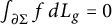 $\int _{\partial \Sigma }f\,dL_g=0$
. Also, (3.7) implies that
 $$ \begin{align} \dfrac{\partial f}{\partial \eta}=2(-\omega_0\cosh^2 r+\omega_i \sinh^2 r) \end{align} $$
is a constant. Using (3.6), the interior component of the weak derivative of
 $\Omega _{r,i}$
gives
 $$ \begin{align} g+\dfrac{1}{2}\sum_{j=1}^m \left(k v_j^2+\vert \nabla^g v_j\vert^2 \right) g-\sum_{j=1}^m dv_j\otimes dv_j-\dfrac12\left(k v_0^2+\vert \nabla^g v_0\vert^2 \right) g+ dv_0\otimes dv_0=0. \end{align} $$
Raising the indices using
 $g^{-1}$
and taking the trace of the above equation yields
 $$ \begin{align} k+\dfrac{k-2}{2}\left(-\vert \nabla^g v_0\vert^2+\sum_{j=1}^m\vert \nabla^g v_j\vert^2\right)+\dfrac{k^2}{2}\left(-v_0^2+\sum_{j=1}^m v_j^2\right)=0. \end{align} $$
Using equation (3.11), we get
 $$ \begin{align} \Delta_g f=\dfrac{4k}{k-2}f. \end{align} $$
Since
 $g\in \tilde {\mathcal {R}}(\Sigma )$
by assumption, we must have
 $f=0$
on
 $\Sigma ^k$
. It follows that the map
 $\Phi $
has image in
 $\mathbb {H}^m$
. Substitute
 $f=0$
back to (3.10) and (3.11), we also find that the map
 $\Phi $
is an isometric immersion into
 $\mathbb {H}^m$
. The remaining steps showing that
 $\Phi $
has image and is an FBMI in fact into
 $B^m(r)$
are completely the same as the spherical case. This completes the proof.
In addition to the theorem above, we see that the proof of Theorem 1.2 can be applied to the functional
 $\Omega _{r,i}$
at little cost. This yields the following converse statement.
Theorem 3.2 Given
 $i\geqslant 1$
, suppose that for some
 $g\in \mathcal {R}(\Sigma ^k)$
, we have either
 $\theta _i(g)<\theta _{i+1}(g)$
or
 $\theta _i(g)>\theta _{i-1}(g)$
. Let
 $V_i(g)$
be the eigenspace of the Steklov eigenvalue
 $\omega _i$
of frequency
 $-k$
:
-
• Suppose there exist
$v_0\in V_0(g)$
and independent
$v_1,\ldots ,v_m\in V_i(g)$
such that:-
(1)
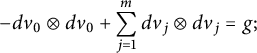
$-dv_0\otimes dv_0+\displaystyle \sum _{j=1}^m dv_j\otimes dv_j=g;$
-
(2)
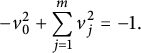
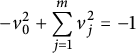
$-v_0^2+\displaystyle \sum _{j=1}^m v_j^2=-1.$
Then, there is some
$r>0$
such that g is an extremal metric for
$\Omega _{r,i}$
in the set
$\mathcal {R}(\Sigma )$
. -
-
• If there exist
$v_0\in V_0(g)$
and independent
$v_1,\ldots ,v_m\in V_i(g)$
such that
$-v_0^2+\displaystyle \sum _{j=1}^m v_j^2=-1$
, the metric g is extremal for
$\Omega _{r,i}$
in the set
$[g]$
for some
$r>0$
.







4 Alternative forms of FBMI characterizing functionals
Here, we present functionals whose critical points, if they exist, correspond to the metrics induced by FBMI of compact manifolds into geodesic balls in
 $\mathbb {S}^m_+$
or
 $\mathbb {H}^m$
.
Let
 $\Sigma ^k$
be a k-dimensional compact manifold with piecewise smooth boundary
 $\partial \Sigma $
as before. We introduce the following two functionals on the set
 $\mathcal R(\Sigma )$
of Riemannian metrics on
 $\Sigma $
:
 $$ \begin{align} \Xi_{r,i}^+(\Sigma,g):=\min\left\lbrace\lambda_0(g,-\tan(r)),\lambda_i(g, \cot(r))\right\rbrace|\Sigma|_g^{2/k},\ i\geqslant 1, \, 0<r<\frac{\pi}{2} \end{align} $$
and
 $$ \begin{align} \Xi_{r,i}^-(\Sigma,g):=\min\{\lambda_0(g, \tanh(r)),\lambda_i(g, \coth(r))\}|\Sigma|_g^{2/k},\, i\geqslant 1, \, r>0. \end{align} $$
Here,
 $\lambda _i(g,\sigma )$
is the ith eigenvalue, arranged in increasing order, of the Robin problem with
 $\sigma \in \mathbb R$
fixed
 $$ \begin{align} \begin{cases} \Delta_gu=\lambda_i(g,\sigma)u\,&\text{ in}\, \Sigma,\\ \dfrac{\partial u}{\partial \eta}=\sigma u\, &\text{ on} \,\partial\Sigma. \end{cases} \end{align} $$
These two functionals are naturally associated with FBMI in the following sense. Let
 $\Phi \colon \Sigma \to \mathbb B^m(r)\subset \mathbb S^m_+$
be an FBMI, given by the
 $\lambda _0(g,-\tan (r))$
and
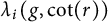 $\lambda _i(g,\cot (r))$
-eigenfunctions, then the energy
 $E[\Phi ]$
satisfies
 $2E[\Phi ]= \Xi _{r,i}^+(\Sigma ,g)$
. Similarly, let
 $\Phi \colon \Sigma \to \mathbb B^m(r)\subset \mathbb H^m$
be an FBMI, given by the
 $\lambda _0(g,\tanh (r))$
and
 $\lambda _i(g,\coth (r))$
-eigenfunctions, then the energy
 $E[\Phi ]$
satisfies
 $2E[\Phi ]= \Xi _{r,i}^-(\Sigma ,g)$
.
Both functionals
 $\Xi _{r,i}^+(\Sigma ,g)$
and
 $\Xi _{r,i}^-(\Sigma ,g)$
admit upper bounds on
 $\mathcal {R}(\Sigma )$
in terms of functionals that have already been analyzed in the literature. Indeed, it follows from their definitions that
 $$ \begin{align*}\Xi_{r,i}^+(\Sigma,g) \leqslant \lambda_i(g, \cot(r))|\Sigma|_g^{2/k} \quad \text{and} \quad \Xi_{r,k}^-(\Sigma,g) \leqslant \lambda_i(g, \coth(r))|\Sigma|_g^{2/k}. \end{align*} $$
Further, we apply [Reference Hassannezhad and Sher17, Proposition 2.6], which implies that
 $\lambda _i(g, \cot (r))<\lambda _i(g,0)=\lambda ^N_i(g)$
, where
 $\lambda ^N_i(g)$
is the ith Neumann eigenvalue. Similarly,
 $\lambda _i(g, \coth (r))<\lambda ^N_i(g)$
. Thus,
 $$ \begin{align*}\Xi_{r,i}^+(\Sigma,g) \leqslant \Lambda^N_i(\Sigma,g) \quad \text{and} \quad \Xi_{r,i}^-(\Sigma,g) \leqslant \Lambda^N_i(\Sigma,g), \end{align*} $$
where
 $\Lambda ^N_i(\Sigma ,g)$
denotes the ith normalized Neumann eigenvalue. It has been proved in [Reference Korevaar22, Reference Li and Yau25] that
 $\Lambda ^N_i(\Sigma ,g)$
is bounded from above in the conformal class
 $[g]$
for any
 $g\in \mathcal R(\Sigma )$
if
 $k>2$
, and bounded from above on
 $\mathcal R(\Sigma )$
if
 $k=2$
. Moreover, in [Reference Li and Yau24], it has been shown that
 $\Lambda ^N_i(\Sigma ,g)$
is bounded from above on the set of metrics of nonnegative Ricci curvature (or more generally Ricci curvature bounded below and diameter bounded above). Summing up, we obtain the following.
Proposition 4.1 The functionals
 $\Xi _{r,i}^+(\Sigma ^k,g)$
and
 $\Xi _{r,i}^-(\Sigma ^k,g)$
are bounded from above on
 $\mathcal F\subset \mathcal R(\Sigma ^k)$
in the following cases:
-
•
$k=2$
and
$\mathcal F=\mathcal R(\Sigma )$
: where C is a positive constant depending on the topology of
$$ \begin{align*}\Xi_{r,i}^\pm(\Sigma^2,g)\leqslant Ci, \end{align*} $$
$\Sigma ^2$
;
-
•
$k>2$
and
$\mathcal F=[g]$
for any
$g\in \mathcal R(\Sigma )$
: where C is a positive constant depending only on k;
$$ \begin{align*}\Xi_{r,i}^\pm(\Sigma^k,g)\leqslant Ci^{2/k}, \end{align*} $$
-
•
$k>2$
and
$\mathcal F$
is the set of metrics satisfying the following inequality: where
$$ \begin{align*}(\mathrm{Ric})d^2\geqslant -a^2, \end{align*} $$
$\mathrm{Ric}$
is a lower bound for the Ricci curvature of
$(\Sigma ^k,g)$
, d is its diameter, and a is a nonnegative constant: where C is a positive constant depending only on k and a.
$$ \begin{align*}\Xi_{r,i}^\pm(\Sigma^k,g)\leqslant Ci^{2/k}, \end{align*} $$





Now, we focus on the case
 $k=2$
and obtain an explicit upper bound of the functional
 $\Xi _{r,1}^+$
as in Theorem 1.4, whose proof is given as follows.
Proof of Theorem 1.4
Take a conformal map
 $u\colon (\Sigma ,g) \to \mathbb B^2(r)$
, where
 $\mathbb B^2(r)$
denotes the geodesic disk in
 $\mathbb S^2_+$
of radius r centered at
 $(1,0,0)$
. There always exists a map u with degree
 $\deg (u)\leqslant 2(\gamma +l)$
(see [Reference Gabard13]). Let
 $x_i,\,i=0,1,2,$
be the coordinate functions of
 $\mathbb R^3$
. Consider
 $u_i=u\circ x_i,\,i=0,1,2$
. One has
 $$ \begin{align} u_0=\cos r,\quad u_1^2+u_2^2=\sin^2r\, \text{ along}\, \partial \Sigma. \end{align} $$
Using the Hersch trick, one can always assume that
 $$ \begin{align*}\int_\Sigma u_i\phi dA_g=0, \, i=1,2, \end{align*} $$
where
 $\phi $
is an eigenfunction of the eigenvalue
 $\lambda _1(g,\sigma )$
for (4.3) with
 $\sigma =\cot (r)$
. Since the map u is conformal, then
 $u^*\delta =f^2 g$
, where f is a positive function on
 $\Sigma $
and
 $\delta $
is the canonical metric on
 $\mathbb B^2(r)$
. It is not hard to verify that
 $$ \begin{align*}\sum_{i=0}^2|\nabla^gu_i|^2_g=2f^2. \end{align*} $$
It follows from the variational characterization that
 $$ \begin{align*}\lambda_0(g,-\tan(r)) \int_\Sigma u_0^2\,dA_g \leqslant \int_\Sigma|\nabla^g u_0|^2_g\,dA_g+\tan(r)\int_{\partial \Sigma}u^2_0\,dL_g \end{align*} $$
and
 $$ \begin{align*}\lambda_1(g,\cot(r)) \int_\Sigma u_i^2\,dA_g \leqslant \int_\Sigma|\nabla^g u_0|^2_g\,dA_g-\cot(r)\int_{\partial \Sigma}u^2_i\,dL_g,\, i=1,2. \end{align*} $$
Summing these inequalities, we get
 $$ \begin{align} \Xi_{r,1}^+(\Sigma,g)&=\min\left\lbrace\lambda_0(g,-\tan(r)),\lambda_1(g, \cot(r))\right\rbrace|\Sigma|_g \\ \nonumber &=\min\left\lbrace\lambda_0(g,-\tan(r)),\lambda_1(g, \cot(r))\right\rbrace \int_\Sigma \sum_{i=0}^2u_i^2\,dA_g \\ \nonumber &\leqslant \lambda_0(g,-\tan(r)) \int_\Sigma u_0^2\,dA_g+\lambda_1(g,\cot(r)) \int_\Sigma \sum_{i=1}^2u_i^2\,dA_g \\ \nonumber &\leqslant \sum_{i=0}^2\int_\Sigma|\nabla^g u_i|^2_g\,dA_g=2\int_\Sigma f^2\,dA_g\leqslant 4\pi(1-\cos r)(\gamma+l), \end{align} $$
where we used
 $\sum _{i=0}^2 u_i^2=1$
in the first inequality and also (4.4) in the second inequality, which yields that
 $$ \begin{align*}\tan(r)\int_{\partial \Sigma}u^2_0\,dL_g=\cot(r)\int_{\partial \Sigma}\sum_{i=1}^2u^2_i\,dL_g .\end{align*} $$
The inequality is proved.
Let
 $\Sigma $
be a topological disk. Then,
 $\gamma =0, \, l=1$
and one gets
 $$ \begin{align*}\Xi_{r,1}^+(\Sigma,g)\leqslant 4\pi(1-\cos r). \end{align*} $$
Let equality hold. Then, we also have equalities at each step in (4.5). This immediately implies that
 $\lambda _0(g,-\tan (r))=\lambda _1(g,\cot (r))$
. Moreover,
 $$ \begin{align*} 0=\Delta_g\sum_{i=0}^2u_i^2&=2\sum_{i=0}^2u_i\Delta_gu_i-2\sum_{i=0}^2|\nabla^gu_i|^2_g\\&=2\lambda_0(g,-\tan(r))u_0^2+2\lambda_1(g,\cot(r))\sum_{i=1}^2u_i^2-2\sum_{i=0}^2|\nabla^gu_i|^2_g, \end{align*} $$
which yields
 $$ \begin{align*} 2f^2=\sum_{i=0}^2|\nabla^gu_i|^2_g&=\lambda_0(g,-\tan(r))u_0^2+\lambda_1(g,\cot(r))\sum_{i=1}^2u_i^2\\&=\lambda_0(g,-\tan(r))=\lambda_1(g,\cot(r)), \end{align*} $$
hence,
 $f\equiv const$
. Then, the metric g is homothetic to
 $\delta $
. In this case, we have
 $|\Sigma |_g=2\pi f^2(1-\cos r)$
. Since
 $ \Xi _{r,1}^+(\Sigma ,g)=4\pi (1-\cos r)$
,
 $$ \begin{align*}\lambda_0(g,-\tan(r))=\lambda_1(g,\cot(r))=\dfrac{2}{f^2}. \end{align*} $$
But then
 $f\equiv 1$
, i.e.,
 $\Sigma =\mathbb B^2(r)$
.
Using the approach developed in [Reference Medvedev28], when studying the behavior of functionals
 $\Theta _{r,i}(\Sigma ^2,g)$
and
 $\Omega _{r,i}(\Sigma ^2,g)$
, we prove the following.
Proposition 4.2 The functionals
 $\Xi _{r,i}^+(\Sigma ^2,g)$
and
 $\Xi _{r,i}^-(\Sigma ^2,g)$
are not bounded from below in
 $[g]$
for any
 $g\in \mathcal R(\Sigma )$
.
Proof Let
 $(\partial \Sigma )_{\varepsilon ^2}$
be the
 $\varepsilon ^2$
-neighborhood of
 $\partial \Sigma $
in
 $(\Sigma ,g)$
. Consider the following family
 $(\varphi _{\varepsilon })_{\varepsilon }$
of nonnegative functions on
 $\Sigma $
such that:
 $$ \begin{align*} supp(\varphi_{\varepsilon}) \subset (\partial\Sigma)_{\varepsilon^2},\quad \varphi_{\varepsilon} < -\log \varepsilon~\text{on}~\Sigma, \quad \text{and}~ \varphi_{\varepsilon}=-\log{\varepsilon}~\text{on}~\partial\Sigma. \end{align*} $$
Consider the following family of conformal metrics
 $(g_{\varepsilon })_{\varepsilon }\in [g]$
, where
 $g_{\varepsilon }:=e^{2\varphi _{\varepsilon }}g$
. Then, for the Robin problem,
 $$ \begin{align*}\begin{cases} \Delta_{g_{\varepsilon}}u=\lambda_i(g_\varepsilon,\sigma) u\,&\text{ in}\, \Sigma,\\ \dfrac{\partial u}{\partial \eta_{\varepsilon,\alpha}}=\sigma u\, &\text{ on} \,\partial\Sigma \end{cases} \end{align*} $$
with
 $\sigma>0$
, the variational characterization yields (see, e.g., [Reference Levitin, Mangoubi and Polterovich23, Formula (3.1.17)])
 $$ \begin{align*}\lambda_i(g_\varepsilon,\sigma) \leqslant \max_{0\neq u\in W}\frac{\displaystyle\int_\Sigma|\nabla^{g_\varepsilon}u|^2_{g_{\varepsilon}}\,dA_{g_{\varepsilon}}-\sigma\int_{\partial \Sigma}u^2\,dL_{g_{\varepsilon}}}{\displaystyle\int_\Sigma u^2\,dA_{g_{\varepsilon}}}, \end{align*} $$
where W is an
 $(i+1)$
-dimensional space in
 $H^1(\Sigma ,dv_{g_{\varepsilon }})$
, which is equivalent to
 $H^1(\Sigma ,dv_g)$
. Using the conformal invariance of the Dirichlet energy for surfaces and the observation that
 $$ \begin{align*}\int_\Sigma u^2\,dA_{g_{\varepsilon}}=\int_{\Sigma\setminus (\partial\Sigma)_{\varepsilon^2}} u^2\,dA_{g}+\int_{(\partial\Sigma)_{\varepsilon^2}} u^2\,e^{2\varphi_{\varepsilon}}dA_{g}>\int_\Sigma u^2\,dA_{g}, \end{align*} $$
since
 $\varphi _{\varepsilon }\geqslant 0$
, we get
 $$ \begin{align*}\lambda_i(g_\varepsilon,\sigma) < \max_{0\neq u\in W}\frac{\displaystyle\int_\Sigma|\nabla^{g}u|^2_{g}\,dA_{g}-\frac{1}{\varepsilon}\sigma\int_{\partial \Sigma}u^2\,dL_{g}}{\displaystyle\int_\Sigma u^2\,dA_{g}}. \end{align*} $$
Taking the minimum over all
 $W\subset H^1(\Sigma ,dv_g)$
of dimension
 $i+1$
from both parts of this inequality and using the variational characterization [Reference Levitin, Mangoubi and Polterovich23, Formula (3.1.17)] once again, we get
 $$ \begin{align} \lambda_i(g_\varepsilon,\sigma) \leqslant \lambda_i(g,\dfrac{1}{\varepsilon}\sigma). \end{align} $$
Consider
 $\Xi _{r,i}^+(\Sigma ,g)$
. The case of
 $\Xi _{r,i}^-(\Sigma ,g)$
is absolutely similar. From its definition, we have
 $$ \begin{align*}\Xi_{r,i}^+(\Sigma,g_{\varepsilon}) \leqslant \lambda_i(g_{\varepsilon}, \cot(r))|\Sigma|_{g_{\varepsilon}}. \end{align*} $$
Take
 $\sigma =\cot (r)$
in (4.6), then the previous inequality becomes
 $$ \begin{align} \Xi_{r,i}^+(\Sigma,g_{\varepsilon}) \leqslant \lambda_i(g, \dfrac{1}{\varepsilon}\cot(r))|\Sigma|_{g_{\varepsilon}}. \end{align} $$
It is not hard to see that
 $|\Sigma |_{g_{\varepsilon }} \to |\Sigma |_{g}$
, as
 $\varepsilon \to 0$
. Indeed,
 $$ \begin{align} &|\Sigma|_{g}<|\Sigma|_{g_{\varepsilon}} =|\Sigma\setminus (\partial\Sigma)_{\varepsilon^2}|_{g}+|(\partial\Sigma)_{\varepsilon^2}|_{g_{\varepsilon}}=|\Sigma\setminus (\partial\Sigma)_{\varepsilon^2}|_{g}+\int_{(\partial\Sigma)_{\varepsilon^2}}e^{2\varphi_{\varepsilon}}dA_{g}\\\nonumber &\leqslant |\Sigma\setminus (\partial\Sigma)_{\varepsilon^2}|_{g}+\frac{1}{\varepsilon^2}\int_{(\partial\Sigma)_{\varepsilon^2}}dA_{g}=|\Sigma\setminus (\partial\Sigma)_{\varepsilon^2}|_{g}+\frac{1}{\varepsilon^2}|(\partial\Sigma)_{\varepsilon^2}|_g. \end{align} $$
In order to compute
 $|(\partial \Sigma )_{\varepsilon ^2}|_g$
, we use the normal coordinates
 $(r,\theta )$
, centered at a point
 $p\in \partial \Sigma $
. Then, it is well-known that
 $g=dr^2+(r-(K(p)/6)r^3+O(r^4))^2d\theta ^2$
, where
 $K(p)$
is the Gauss curvature of
 $(\Sigma ,g)$
at p. Then, the area with respect to g of the part of the disk centered at p of radius
 $\varepsilon ^2$
containing in
 $\Sigma $
is less than
 $$ \begin{align*}2\pi\int_0^{\varepsilon^2}\left(r-\frac{K(p)}{6}r^3+O(r^4)\right)\,dr=\pi\varepsilon^4+o(\varepsilon^8), \text{ as } \varepsilon\to 0. \end{align*} $$
Let
 $\partial _p\Sigma $
denote the connected component of
 $\partial \Sigma $
, containing p. Hence, because of the overlapping, the
 $\varepsilon ^2$
-tubular neighborhood of
 $\partial _p\Sigma $
has area with respect to g less than
 $$ \begin{align*}\left(\pi\varepsilon^4+o(\varepsilon^8)\right)|\partial_p\Sigma|_g,\text{ as } \varepsilon\to 0. \end{align*} $$
Hence,
 $|(\partial \Sigma )_{\varepsilon ^2}|_g<\pi \varepsilon ^4|\partial \Sigma |_g+o(\varepsilon ^8)$
, as
 $\varepsilon \to 0$
, where
 $|\partial \Sigma |_g$
is the total length of the boundary with respect to g. Coming back to (4.8), we get
 $$ \begin{align*}|\Sigma|_{g}<|\Sigma|_{g_{\varepsilon}}=|\Sigma\setminus (\partial\Sigma)_{\varepsilon^2}|_{g}+\pi\varepsilon^2|\partial\Sigma|_g+o(\varepsilon^6), \text{ as } \varepsilon\to 0 \end{align*} $$
and we obtain the desired by the squeezing theorem.
Further,
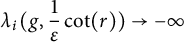 $\lambda _i(g, \dfrac {1}{\varepsilon }\cot (r))\to -\infty $
, as
 $\varepsilon \to 0$
by [Reference Hassannezhad and Sher17, Proposition 2.6]. Hence, coming back to (4.7), we get
 $$ \begin{align*}\Xi_{r,i}^+(\Sigma,g_{\varepsilon}) \to -\infty,~\text{ as }~\varepsilon\to 0. \end{align*} $$
We now investigate the critical points for these two functionals. We start with properties of Laplacian eigenvalues with Robin boundary conditions. Following the approach in [Reference Lima and Menezes26], we can prove the following lemma.
Lemma 4.3 Let
 $\Sigma ^k$
be a compact manifold with piecewise-smooth boundary. Suppose
 $(g_t)_t$
is a family of Riemannian metrics analytically indexed by
 $t\in (-\epsilon ,\epsilon )$
with
 $g_0=g$
. Denote
 $g_t^b$
the induced metric on
 $\partial \Sigma $
with
 $g^b=g_0^b$
. For each prescribed
 $\sigma \in \mathbb {R}$
, let
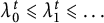 $\lambda _0^t\leqslant \lambda _1^t\leqslant \dots $
be the Laplacian eigenvalues such that
 $$ \begin{align} \begin{cases} \Delta_{g_t} u=\lambda_i^t u\ &\mathrm{in}\ \Sigma, \\ \dfrac{\partial u}{\partial \eta^t}= \sigma u\ &\mathrm{on}\ \partial\Sigma. \end{cases} \end{align} $$
Denote
 $E_i(g_t,\sigma )$
the eigenspace of
 $\lambda _i^t$
satisfying (4.9). Then, the following hold:
-
(1) Each eigenvalue
$\lambda _i^t$
is Lipschitz in t, and admits a weak derivative in t. -
(2) Suppose a family of metrics
$(g_t)$
has derivatives
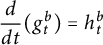
$\dfrac {d}{dt}(g_t)=h_t$
on
$\Sigma $
and
$\dfrac {d}{dt}(g^b_t)=h_t^b$
on
$\partial \Sigma $
. Denote
$dA_t$
and
$dL_t$
the measures, induced by
$g_t$
on
$\Sigma $
and
$\partial \Sigma $
, respectively. We can find an
$L^2(\Sigma ,dA_t)$
-normalized functions
$\phi _i^t$
such that the weak derivative of
$\lambda _i^t$
is given by the following formula: (4.10)
$$ \begin{align} \begin{aligned} -\int_{\Sigma} \left\langle d\phi_i^t\otimes d\phi_i^t+\dfrac{1}{4} \Delta_{g_t} (\phi_i^t)^2 g_t, h_t \right\rangle_t dA_t-\dfrac{\sigma}{2}\int_{\partial\Sigma}(\phi_i^t)^2\langle h_t^b,g_t^b \rangle_t dL_t. \end{aligned} \end{align} $$




From the lemma above, we see that for a smooth family
 $(g_t)_t$
of metrics, the functions
 $\Xi ^+_{r,k}(g_t)$
and
 $\Xi ^+_{r,k}(g_t)$
are Lipschitz, hence differentiable almost everywhere. To study the critical metrics of the functionals
 $\Xi ^+_{r,k}$
and
 $\Xi ^-_{r,k}$
, we need the following statement on the weak derivatives of the normalized Laplace eigenvalues and of these functionals.
Lemma 4.4 For a smooth family
 $(g_t)_{t\in (-\varepsilon ,\varepsilon )}$
of Riemannian metrics, let
 $h_t=\dfrac {d}{dt} (g_t)$
. The weak derivative of the following normalized Laplace eigenvalue
 $$ \begin{align} \lambda_i\left(g_t, \sigma \right)\vert\Sigma\vert_{g_t}^{2/k},\ i\geqslant 0 \end{align} $$
is given by
 $$ \begin{align} \begin{aligned} Q_{t,i}(\sigma)(u^t)= & -A_t^{(2-k)/k} \bigg( \int_{\Sigma}\left\langle A_t\left( du^t\otimes du^t+\dfrac{1}{4}\Delta_{g_t}(u^t)^2g _t\right)-\dfrac{\lambda_i^t}{k}g_t,h_t\right\rangle_t d\mu_t\\ & +\dfrac{\sigma A_t}{2}\int_{\partial\Sigma} (u_t)^2 \langle g^b_t,h^b_t\rangle_t d\nu_t \bigg) \end{aligned} \end{align} $$
for some
 $L^2(\Sigma ,g_t)$
-normalized
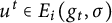 $u^t\in E_i(g_t,\sigma )$
, and
 $A_t=\vert \Sigma \vert _{g_t}$
. Given any fixed
 $i\geqslant 1$
, the functions
 $\Xi ^+_{r,i}(g_t)$
and
 $\Xi ^-_{r,i}(g_t)$
are differentiable almost everywhere, and their weak derivative formulas can be directly obtained from (4.12).
Proof Recall that
 $$ \begin{align*} \dfrac{d}{dt}\left(\vert \Sigma\vert_{g_t} \right)=\dfrac{1}{2}\int_{\Sigma}\langle g_t,h_t\rangle_t d\mu_t. \end{align*} $$
Combining this with the formula (4.10), a direct computation gives the formula of the weak derivatives of the normalized Laplace eigenvalues (4.12).
For
 $i\geqslant 1$
given, the two normalized Laplace eigenvalues in the formula of
 $\Xi ^+_{r,i}(g_t)$
(also of
 $\Xi ^-_{r,i}$
) are both differentiable almost everywhere. Fix
 $t_0$
such that the two normalized eigenvalues are both differentiable. The derivative of
 $\Xi ^+_{r,i}(g_t)$
at
 $t=t_0$
is then given by
 $Q_{t_0,0}(-\tan (r))(u^{t_0}_0)$
(resp.
 $Q_{t,i}(\cot (r))(u_1^{t_0})$
) if
 $\lambda _0(g_{t_0},-\tan r)$
(resp.
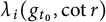 $\lambda _i(g_{t_0},\cot r)$
) is smaller. For the case these two eigenvalues are equal, we have
 $$ \begin{align*} \dfrac{d}{dt}\bigg\vert_{t=t_0}\Xi^+_{r,i}(g_t)=\min\lbrace Q_{t_0,0}(-\tan(r))(u^{t_0}_0), Q_{t,i}(\cot(r))(u_1^{t_0})\rbrace, \end{align*} $$
where
 $u_0^{t_0}\in E_0(g_{t_0},-\tan r)$
and
 $u_1^{t_0}=E_i(g_{t_0}, \cot r)$
. A similar statement also holds for the functional
 $\Xi ^-_{r,i}(g_t)$
.
With the result above, we shall be able to complete the proof of Theorem 1.3.
Proof of Theorem 1.3
We first prove the part of theorem about when the functionals
 $\Xi ^+_{r,i}$
and
 $\Xi ^-_{r,i}$
have critical metrics (if any). For
 $u\in E_i(g,\sigma )$
, define the mapping
 $$ \begin{align*} T(u,\sigma):=\lbrace(\tau^k(u),F(u,\sigma))\in S^2(\Sigma)\times S^2(\partial\Sigma) \rbrace, \end{align*} $$
where
 $$ \begin{align*} &\tau^k(u):= A\left(du\otimes du +\dfrac{1}{4}\Delta_g(u^2)g\right)- \dfrac{\lambda_i}{k}g,\\ & F(u,\sigma):=\dfrac{A\sigma}{2}u^2 g^b. \end{align*} $$
Here, g is a critical metric of
 $\Xi ^+_{r,i}$
by assumption and recall that
 $A=\vert \Sigma \vert _g$
. We use Lemma 4.4 and argue as in the Robin eigenvalue case in Section 2.1. We can show for any
 $$ \begin{align*}(h_1,h_2)\in L^2(S^2(\Sigma),g)\times L^2(S^2(\partial\Sigma),g),\end{align*} $$
there exist
 $L^2(\Sigma ,g)$
-normalized functions
 $u,v\in E_0(g,-\tan r)\cup E_i(g,\cot r)$
such that
 $$ \begin{align} \langle T(u),(h_1,h_2)\rangle \langle T(v),(h_1,h_2)\rangle \leqslant 0. \end{align} $$
Let
 $\widehat {C}$
be the convex hull generated by
 $T(u_0,-\tan r)$
and the following set
 $$ \begin{align*} K_i=\lbrace T(u,\cot r):u\in E_i(g,\cot r), \Vert u\Vert_{L^2(\Sigma,g)}=1 \rbrace. \end{align*} $$
Note that the convex hull
 $\widehat {C}$
is compact.
Then, we must have
 $(0,0)\in \widehat {C}$
. Otherwise, as
 $\hat {C}$
is compact, there exists some
 $$ \begin{align*}(h_1,h_2)\in L^2(S^2(\Sigma),g)\times L^2(S^2(\partial\Sigma),g)\end{align*} $$
such that
 $$ \begin{align*} \inf_{(\tau,F)\in\widehat{C}}\left\langle (\tau,F),(h_1,h_2)\right\rangle>\epsilon>0. \end{align*} $$
This and (4.13) lead to a contradiction.
When g is a critical metric of
 $\Xi ^-_{r,i}$
, an analogous argument shows the convex hull generated by
 $T(u_0,\tanh r)$
and the set
 $$ \begin{align*} \lbrace T(u,\coth r): u\in E_i(g,\coth r), \Vert u\Vert_{L^2(\Sigma,g)}=1 \rbrace \end{align*} $$
also contains the point
 $(0,0)$
.
Then, there exist nonnegative constants
 $\lbrace t_{\alpha }\rbrace _{\alpha =0}^m$
with
 $\displaystyle \sum _{\alpha =0}^m t_{\alpha }=1$
and
 $L^2$
-normalized
 $u_0\in E_0(g,\sigma _0)$
and
 $\lbrace u_j \rbrace _{j=1}^m$
in
 $E_i(g,\sigma _1)$
such that
 $$ \begin{align} \left\{ \begin{aligned} & \sum_{\alpha=0}^m t_{\alpha}\tau^k(u_{\alpha})=0\ \mathrm{on}\ \Sigma,\\ & \sum_{\alpha=0}^m t_{\alpha} F(u_{\alpha})=0 \ \mathrm{on}\ \partial\Sigma, \end{aligned} \right. \end{align} $$
where
 $\sigma _0=-\tan r$
and
 $\sigma _1=\cot r$
for
 $\Xi ^+_{r,i}$
, and
 $\sigma _0=\tanh r$
and
 $\sigma _1=\coth r$
for
 $\Xi ^-_{r,i}$
. The second line of (4.14) never holds for
 $\Xi ^-_{r,i}$
, since
 $\coth r$
and
 $\tanh r$
are both strictly positive when
 $r>0$
. Thus, (4.2) has no critical point. The functional (4.1) can only have critical points when the equality (1.2) holds. If this is not the case, the derivative of
 $\Xi ^+_{r,i}(\Sigma ,g_t)$
near
 $t=0$
is induced by the branch
 $\lambda _0(g_t,-\tan r)\vert \Sigma \vert ^{2/k}_{g_t}$
if
 $$ \begin{align*}\lambda_0(g_0,-\tan r)<\lambda_i(g_0,\cot r)\end{align*} $$
and by
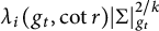 $\lambda _i(g_t,\cot r)\vert \Sigma \vert ^{2/k}_{g_t}$
if
 $$ \begin{align*}\lambda_0(g_0,-\tan r)>\lambda_i(g_0,\cot r).\end{align*} $$
First suppose that this derivative is induced by
 $\lambda _0(g_t,-\tan r)\vert \Sigma \vert ^{2/k}_{g_t}$
. Note that
 $\lambda _0$
is always simple and always differentiable, so the derivative of
 $\lambda _0(g_t,-\tan r)\vert \Sigma \vert ^{2/k}_{g_t}$
at
 $t=0$
shall vanish. The derivative of
 $\Xi ^+_{r,i}(g_t)$
at
 $t=0$
is given by
 $Q_{0,0}(-\tan (r))(u^{0}_0)$
for some
 $L^2(\Sigma ,g_0)$
-normalized
 $u^0_0\in E_0(g_0,-\tan r)$
. From (4.12), this is impossible for setting
 $h_0^b=g_0^b$
and
 $\Vert h_0\Vert _{L^2(S^2(\Sigma ),g_0)}$
sufficiently small. Now suppose the other case that the derivative is induced by
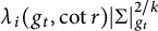 $\lambda _i(g_t,\cot r)\vert \Sigma \vert ^{2/k}_{g_t}$
. Use an argument as in the beginning of this proof on the convex hull generated by
 $K_i$
instead of
 $\hat {C}$
, one would get
 $(0,0)\in K_i$
, which is clearly impossible. In summary, the critical points of this functional can only occur when the two branches defining the functional are equal, so each breach gives one of the one-sided derivatives at
 $t=0,$
for some chosen variation
 $\{g_t\}$
.
Denote this common Laplace eigenvalue by
 $\lambda $
from now. The divergence theorem applied with
 $\sigma =-\tan r<0$
shows
 $\lambda>0$
. From above, we can assume now
 $0<t_{\alpha }<1$
for all
 $0\leqslant \alpha \leqslant m$
. Define
 $v_{\alpha }=\sqrt {t_{\alpha }}u_{\alpha }$
. The first line of (4.14) yields
 $$ \begin{align} A \sum_{\alpha=0}^m \left[ dv_{\alpha}\otimes dv_{\alpha}-\dfrac{1}{2}(\vert \nabla v_{\alpha}\vert_g^2-\lambda v_{\alpha}^2 )g \right]-\dfrac{\lambda}{k}g=0. \end{align} $$
Taking trace of the equation above, we obtain
 $$ \begin{align} A\sum_{\alpha=0}^m\vert \nabla v_{\alpha}\vert_g^2\left(1-\dfrac{k}{2} \right)=\dfrac{-k\lambda}{2}\left(A\sum_{\alpha=0}^m v_{\alpha}^2-\dfrac{2}{k}\right). \end{align} $$
Let us first assume
 $k>2$
, using the same trick as before, define
 $$ \begin{align*} f=\dfrac{4\lambda}{k-2}\sum_{\alpha=0}^m v_{\alpha}^2-\dfrac{4\lambda}{A(k-2)}. \end{align*} $$
Then, f is a Laplace eigenfunction with negative eigenvalue
 $\dfrac {4\lambda }{2-k}$
. Moreover, the second line of (4.14) gives
 $$ \begin{align} (-\tan (r)) v_0^2 +\cot r\sum_{j=0}^m v_j^2\equiv 0,\ \mathrm{on}\ \partial\Sigma. \end{align} $$
Thus, we have
 $\dfrac {\partial f}{\partial \eta }\equiv 0$
on
 $\partial \Sigma $
. Hence, on
 $\Sigma $
, we see
 $$ \begin{align} \sum_{\alpha} v_{\alpha}^2-\dfrac{1}{A}\equiv 0. \end{align} $$
For the special case
 $k=2$
, (4.16) immediately gives (4.18).
Combining (4.18) with (4.17), we find
 $$ \begin{align} v_0=\dfrac{1}{\sqrt{A}}\cos r,\ \mathrm{and}\ \sum_{j=0}^m v_j^2=\dfrac{1}{A}\sin^2 r\ \mathrm{on}\ \partial\Sigma. \end{align} $$
Substitute (4.18) and (4.19) back to (4.15), we get
 $$ \begin{align*} 1-\dfrac{\lambda}{k}g(\eta,\eta)=0. \end{align*} $$
Since
 $\eta $
is a unit norm vector field for g, we necessarily obtain
 $\lambda =k$
. This shows the map
 $\sqrt {A}(v_0,v_1,\ldots ,v_m)$
is an isometric immersion from
 $(\Sigma ,g)$
into
 $\mathbb {S}^m_+$
. It follows analogously as the previous case that the immersion is actually an FBMI into
 $\mathbb B^m(r)$
.
Acknowledgements
The authors would like to thank Iosif Polterovich and Mikhail Karpukhin for their comments on a preliminary version of the manuscript, as well as the anonymous referees for their valuable suggestions and constructive feedback. The work of the second author is an output of a research project implemented as part of the Basic Research Program at the National Research University Higher School of Economics (HSE University).



