Introduction

Remote-sensing measurements show that the surface elevation of polar ice sheets varies with time in response to climate change. Short-term variations are caused by seasonal or interannual variations of surface weather conditions through the firn compaction process, while long-term changes are generally considered to be due to ice dynamic response to past mass-balance states of the ice sheet (Reference Zwally and LiZwally and Li, 2002).

Within an ice sheet changes to the flow properties controlled by naturally developed crystallographic structure may affect its flow (Reference BuddBudd, 1969). For example, results from the Law Dome deep borehole (Dome Summit South (DSS)) in East Antarctica have shown that a strong single-maximum fabric is preserved in the impurity-rich ice layer that was deposited during the Last Glacial Maximum (LGM), leading to a flow rate approximately one order of magnitude greater than in adjacent layers (Reference Morgan, Wookey, Li, van Ommen, Skinner and FitzpatrickMorgan and others, 1997, Reference Morgan, van Ommen, Elcheikh and Jun1998; Li and others, 1998). A consequence of the different flow rates exhibited by this ice would be a varying vertical velocity profile as the layer descended through the ice sheet. It is necessary to understand and assess the role of the variation of crystal anisotropy with thickness change in the interpretation of remote-sensing results.

The time needed for an ice particle to travel from the surface to a particular depth within an ice sheet is a function of the change in ice thickness with time, the accumulation rate, the ice-sheet geometry and the ice rheology. Once the age–depth relation is known, the ice-sheet history may be reconstructed (e.g. Reference Bolzan, Waddington, Alley and MeeseBolzan and others, 1995; Reference Cutler, Raymond, Waddington, Meese and AlleyCutler and others, 1995). The accuracy of reconstructions of accumulation and surface elevation is dependent on the divide migration, temperature and ice rheology. Investigation into the ice-divide position shows it appears to be most sensitive to the position of the ice-sheet margins, the accumulation rate, the temperature profile and the ice-stiffness profile (Reference Azuma and Goto-AzumaAnandakrishnan and others, 1994).

In this study, an ice-flow model incorporating crystal anisotropy properties is developed and applied to Law Dome at the location of the DSS deep borehole. The results are used to reconstruct the history of the ice sheet, with emphasis on the effect of variation in anisotropic flow properties (ice rheology) on the ice-sheet surface elevation change. Annual-layer thickness data from the DSS ice core (Reference Morgan, Wookey, Li, van Ommen, Skinner and FitzpatrickMorgan and others, 1997; Reference Van Ommen, Morgan and CurranVan Ommen and others, 2004) are used as the model input.

Model Description

A one-dimensional ice-flow model incorporating crystal anisotropic properties is developed based on the theory and method used by Reference Cutler, Raymond, Waddington, Meese and AlleyCutler and others (1995) for Greenland ice-core studies.

We consider the ice-sheet profile as a Reference VialovVialov (1958) steady-state profile (Fig. 1) as described by Reference PatersonPaterson (1994, p. 243) in detail. At the ice-sheet divide, this shape gives the following relationship between the ice-sheet thickness H and the surface vertical velocity Vs at time t.

Fig. 1.

A simple profile of ice-sheet flow. Z is vertically upward, X horizontally along the ice-sheet flow from the divide, b is surface accumulation rate, α is ice-sheet surface slope, H is ice thickness at the divide, L is the half-width of the ice sheet, and U and V represent the horizontal and vertical velocity components, respectively. Ice-flow trajectories are shown by dashed lines. Annual layers with depth near the ice divide are also shown.

where K is a function of flow-law exponent n, temperature parameter A, ice density ρ, gravity acceleration g and the half-width of the ice sheet L. Based on the assumption that the surface geometry and bedrock remain unchanged over the time interval of interest and that A is independent with the time, K =1280 (μ⁷ a)^1/8 is then determined from the present ice-sheet condition (H =1220 m, Vs = 0.68 ma^–1, taken from Reference Van Ommen, Morgan and CurranVan Ommen and others, 2004) by choosing n = 3 (e.g. Reference Jacka and BuddGlen, 1958; Reference BuddBudd, 1969; Reference HookeHooke, 1981; Reference Budd and JackaBudd and Jacka, 1989).

The equation used to determine the ice-sheet thickness change is the continuity equation that expresses the law of mass conservation of a moving continuum. We consider the DSS site (Reference Morgan, Wookey, Li, van Ommen, Skinner and FitzpatrickMorgan and others, 1997) as an ice column near the ice divide of the ice sheet (Fig. 1) and assume that

• 1. the basal ice is frozen to the bed

• 2. the surface slope of the ice sheet is small so that Uα is neglected, where U and α are surface horizontal velocity and slope, respectively.

  The continuity equation (Reference PatersonPaterson, 1994, p. 258) can be simplified as

  

  (2)

  where ∂H/∂t is the ice-thickness change with time (t) over a fixed point of the bedrock, b is surface accumulation rate (positive) and Vs is surface vertical velocity (negative).

  We further assume that:

• 3. the ice is incompressible

• 4. the shape of the horizontal-velocity/depth profile varies only slowly with x

• 5. vertical velocity shape is constant with time.

Based on assumptions (i–v) above, the vertical velocity at time t and depth z is given as

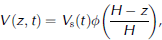
and

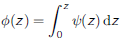
where U(z) and represent the depth-dependent horizontal velocity and the depth-averaged horizontal velocity, respectively. The vertical-velocity shape (φ) accounts for the vertical transport of material within the ice sheet and varies from 1 at the surface to 0 at the base of the ice. is a function of depth which gives the shape of the horizontal velocity as a function of the depth and may be calculated from the flow law (Reference ReehReeh, 1988; Reference Budd and JenssenBudd and Jenssen, 1989). The relationship between and the flow law is discussed below.

Fundamental to our understanding of the dynamics of ice sheets is the rheological flow law (constitutive relation) for ice, i.e. the relation between strain rate and stress. For isotropic ice flow, the most commonly used relation between strain rate and stress is the Glen flow law (Reference HookeGlen, 1955, Reference Jacka and Budd1958)

where έ ij is the strain-rate tensor, the deviatoric stress tensor and A(T) the temperature-dependent parameter. I ₂(τ) is the second invariant of the deviatoric stress tensor

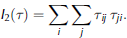
For anisotropic ice flow, some attempts have been made to incorporate the effects of anisotropy into the constitutive relation. One approach is to establish a new theoretical expression for the constitutive relation which includes anisotropy (e.g. Reference LileLile, 1978; Reference Doake and WolffDoake and Wolff, 1985; Reference Lliboutry and DuvalLliboutry and Duval, 1985; Reference Anandakrishnan, Alley and WaddingtonAzuma and Goto-Azuma, 1996; Reference Mangeney, Califano and CastelnauMangeney and others, 1996, Reference Paterson1997; Reference Goldsby and KohlstedtGoldsby and Kohlstedt, 2001). Another approach, a simpler procedure accounting for anisotropy, is to modify Glen’s flow law by introducing an enhancement factor (e.g. Reference Russell-Head and BuddRussell-Head and Budd, 1979; Reference Dahl-JensenDahl-Jensen, 1985; Reference ReehReeh, 1988; Reference Wang and WarnerWang and Warner, 1998; Reference Wang, Warner and BuddWang and others, 2002). The enhancement factor, defined as the ratio of the strain rate for anisotropic ice to the strain rate for isotropic ice, can be derived from laboratory experiments (e.g. Reference Budd and JenssenRussell-Head and Budd, 1979; Reference Jacka and BuddJacka and Budd, 1989; Li and others, 1996) and also from field observations (e.g. Reference Budd and JenssenRussell-Head and Budd, 1979; Reference Dahl-JensenDahl-Jensen, 1985; Reference Wang, Warner and BuddWang and others, 2002) where an increase in enhancement factor is associated with strengthening of a near-vertical single-maximum fabric (e.g. Fig. 2b).

Fig. 2.

Depth profiles of (a) temperature parameter A(T) (bar^–3 a^–1); (b) enhancement factor E and selected fabric diagrams (Reference Wang, Warner and BuddWang and others, 2002); (c) horizontal velocity U (m a^–1); (d) horizontal-velocity shape; and (e) vertical-velocity shape φ, for various ice rheologies: (i) temperature-dependent with varied fabrics (solid line), (ii) temperature-dependent with unvaried fabrics (dashed line), and (iii) temperature-independent with unvaried fabrics (dotted line). The LGM depth is marked in (b). φ is rescaled to a relative depth for the model calculations.

In this study, we follow our previous study (Reference Wang, Warner and BuddWang and others, 2002) by using an enhancement factor E to account for the effect of ice structure (ice fabric, crystal size and dust). The ice flow is assumed to be plane strain flow, and the flow relations for components of shear and compression are:

where the x coordinate is in the direction of flow, the y coordinate is transverse to the flow and the z coordinate is the vertical direction. τ represents the effective shear stress and is taken as

on the assumption made in Equations (8–11) that the ice flow corresponds to a confined vertical compression stress combined with a horizontal shear stress. denotes the vertical compressive deviatoric stress. Shear stress τ_xz is calculated by

in terms of ice density ρ, gravitative acceleration g, the depth of the ice sheet (H – z) and surface slope α.

From Equations (8), (9) and (12), the flow relation can be rewritten as

For a chosen A(T) and E, Equation 1 is solved iteratively for the shear strain rate έ xz by taking n = 3. Horizontal velocity is then calculated by integrating shear strain rate

Inserting Equations (8) and (15) into Equation 1, becomes

which indicates that (or φ in Equation 1) is dependent on the depth distributions of enhancement factor, temperature and stresses. For the isothermal ice with unvarying fabrics (i.e. E and A are constants), if τ_xz is the only non-zero stress component (i.e. laminar flow), the depth-averaged horizontal velocity is (Reference PatersonPaterson, 1994, p. 251–252)

therefore and φ vary only as a function of the depth z and the flow-law exponent n and can be calculated from

Calculations

The model described above was applied to the DSS site to reconstruct the ice-sheet history of accumulation rate, ice thickness and the rate of change in ice thickness.

Since the present-day accumulation rate at DSS (0.68 m a^–1 ice equivalent) is high compared with most other polar sites, we took a 20 year time-step (Δt = 20 years) instead of the 50 year step used for Greenland ice-core studies (e.g. Reference Cutler, Raymond, Waddington, Meese and AlleyCutler and others, 1995) to establish the annual-layer depth profile (ALDP) using the smoothed layer thickness–depth relation given by Reference Morgan, Wookey, Li, van Ommen, Skinner and FitzpatrickMorgan and others (1997) with the updated parameters (in ice equivalent) given by Reference Van Ommen, Morgan and CurranVan Ommen and others (2004) as:

where d = H ₀ – z (m) is the depth from the ice-sheet surface, b ₀ = 0.68 (ma^–1) is the present-day accumulation rate, D = 1029.2 (m) is the intercept on the depth-axis above-break linear region, H ₀ = 1218.6 (m) is the effective ice-sheet thickness, dbreak = 2D – H ₀ = 839.8 (m) is the break-point depth at which the vertical strain rate starts to decrease, and tbreak = (D/b ₀) ln[D/(H₀ – D)] (years) is time at the break point.

This profile from the surface to the depth below the LGM/Holocene transition with age about 13 000 years BP was used as the model input. For given values of (i) time-step Δt (20 years), (ii) initial vertical velocity distribution V(z) = ALDP, and (iii) vertical-velocity shape profile φ calculated based on the different ice rheologies, Equations (1–3) were used to reconstruct the ice-sheet history such as accumulation rate b(t), ice thickness H(t) and the change rate in ice thickness ∂H/∂t (t). In order to obtain stable results, we coupled the forward and backward calculations using iterative technique. We started with a constant ice thickness of 1220m to calculate a corresponding accumulation history by unstraining the annual layers from the DSS core (moving backward in time (Equations (2) and (3)). This accumulation history was then used to calculate a new ice-thickness history by running the model forward in time (Equations (1) and (2)). A new accumulation history was then calculated using the updated ice thickness by running the model backward in time again, and this process was repeated until both the accumulation and ice-thickness history converged (see Reference Cutler, Raymond, Waddington, Meese and AlleyCutler and others, 1995, Fig. 3, for details).

Fig. 3.

Left panel shows the reconstructed history of (a) surface accumulation rate b, (b) ice thickness H and (c) ice-thickness change rate dH/dt, for the three cases presented in Figure 2. Right panel shows the differences of case (i) (solid line) and case (iii) (dotted line) with case (ii), respectively.

It is obvious that the results of the reconstructed ice-thickness and/or accumulation history using this model depend on the input of the annual-layer thickness profile and the shape function of vertical velocity (Equation 1). The vertical-velocity shape is based on the ice rheology as described previously.

To investigate the effect of the ice rheology on the ice-sheet surface elevation change, the model was run for three cases with the following ice rheologies:

1. Temperature-dependent with varied fabrics: temperature parameter A(T) and enhancement factor E (Fig. 2, solid lines) are taken from the previous study results based on the borehole measurements (Reference Wang, Warner and BuddWang and others, 2002, Fig. 2). The enhancement factor becomes significant at about 40 m depth and then maintains a value of about 5 between 600 and 1000 m. E decreases below 1000m to values ~1 at 1100 m. This variation is accompanied by changes in the ice fabric, from single-maximum to multi-maximum, associated with the increasing crystal size due to ice recrystallization and possible shear stress relaxation near the bedrock. In addition, in the lower part of the borehole, there is a narrow spike of very high values of enhancement factor which is associated with ice from the LGM. This ice has relatively high levels of dust and chemical impurities and small crystals with strong single-maximum fabrics (Li and others, 1996; Reference Morgan, Wookey, Li, van Ommen, Skinner and FitzpatrickMorgan and others, 1997).

2. Temperature-dependent with unvaried fabrics: the temperature parameter A(T) is taken from the borehole temperature observations, and a constant enhancement factor E is chosen in order to obtain the borehole surface horizontal velocity (Fig. 2, dashed lines).

3. Temperature-independent (isothermal) with unvaried fabrics: a constant enhancement factor E is taken as the same value as case (ii), and a constant temperature parameter A is chosen in order to match the observed surface velocity (Fig. 2, dotted lines).

The corresponding horizontal-velocity shape and vertical-velocity shape φ resulting from the three ice rheologies assumed above are shown in Figure 2d and e. It should be mentioned that υ (or φ) is independent of any constant value of A or E (see Equation 1).

Results and Discussion

We discuss three different ice-flow scenarios: ‘temperature-dependent with varied fabrics’ (‘enhanced’); ‘temperature-dependent with unvaried fabrics’ (‘non-enhanced’); and ‘temperature-independent (isothermal) with unvaried fabrics’ (‘isothermal non-enhanced’).

Figure 3a₁–c₁ show the reconstructed history of accumulation rate, ice thickness and the rate of ice-thickness change, respectively, at the DSS site. Different line types indicate the results from the model using the three different vertical-velocity shape functions (φ) presented in Figure 2e. To show the differences between each case, Figure 3a₂–c₂ plot the corresponding residues compared to the ‘non-enhanced’ case.

Comparison of the three cases in Figure 3a₁–c₁ shows the three vertical-velocity shapes generate similar values at the beginning and end times but with significant differences in between. This characteristic is due to the nature of the shape function that has a value of 1 at the surface and 0 at the bottom of the ice sheet (Fig. 2e), although the accumulation rate and ice thickness at present are prescribed during the calculations. The maximum differences occur at 4000– 7000 years BP (Fig. 3a₂–c₂) where the accumulation rate increases most dramatically (Fig. 3a₁).

As shown in Figure 3b₁, our calculations for all three cases predict an ice-thickness reduction (about 350 m for the ‘enhanced’ case) during the last glacial period (>10 000 years BP). Ice thickness increases through the glacial/Holocene transition, reaching a maximum of around 2500 BP. The thickness is slightly greater (about 40 m for the ‘enhanced’ case) than at present. The variation generally follows the accumulation trend (Fig. 3a₁) where the accumulation rate continuously increases from the glacial where it is <10% of the present rate to the maximum at about 2500 BP with the rate about 20% higher than the present.

Reconstructed accumulation rates for ‘enhanced’ and ‘isothermal non-enhanced’ are approximately 0.3 and 0.2 ma^–1 lower than for the ‘non-enhanced’ case, yielding ice thicknesses about 140 and 60m lower (Fig. 3a₂ and b₂). The differences are most severe in the ice-thickness change rate (Fig. 3c₁ and c₂). The maximum thickening rate for the ‘non-enhanced’ case is around 0.04ma^–1, with differences of about 0.08 and 0.03 ma^–1 for the ‘enhanced’ and ‘isothermal non-enhanced’ cases, giving about 50–100% differences. The ranges of variation in ice-thickness change rate (Fig. 3c₁) are about 0.1 (enhanced), 0.06 (isothermal non-enhanced) and 0.04 (non-enhanced), indicating that the ‘enhanced’ case is the most sensitive to surface climatic change. In other words, the model without consideration of the enhancement due to the developed crystal anisotropy is more likely to give the results with more modest variations.

The calculation shown in Figure 3 assumes that the shape function is not altered by the evolving temperature and other factors affecting ice softness. This is not always the case in natural ice sheets, and it has been widely found over Antarctica and Greenland ice sheets that the ice deposited during the last glacier cycle contains a high amount of impurities that retard the normal evolution of the crystal structure, resulting in ‘unusual’ flow properties (cf. Reference PatersonPaterson, 1991; Li and others, 1998). At DSS, borehole inclination measurements indicate that the shear strain rate at the LGM depth (~1113 m) is ten times greater than in the adjacent ice layers (Reference Morgan, van Ommen, Elcheikh and JunMorgan and others, 1998), i.e the ice has much higher ‘unusual’ enhancement (Fig. 2b). To estimate the importance of this unusual softness, we performed a test by creating a layer with an arbitrary thickness of 25m at 1000m depth (Fig. 4a), where the enhancement for normal ice reaches the maximum (Fig. 2b). The magnitude of the enhancement for the peak was scaled according to the present value of the enhancement for the LGM ice layer with respect to that for normal ice. The corresponding shape functions of velocity are shown in Figure 4b and c. As shown by dashed curves in Figure 5, the shear layer produces notable differences in the time interval between about 3000 and 5000 BP, with larger spikes (magnitudes five to ten times) around 4000 BP. The impurity-rich LGM ice with the abnormally high flow enhancement at DSS (Fig. 2b) is about 10m thick and covers a roughly 10 000 year timespan (Reference Morgan, van Ommen, Elcheikh and JunMorgan and others, 1997). Since this ice layer would have covered larger and varying depth intervals while moving from the surface to bedrock along its trajectory, the shape function φ is actually time-dependent. Our analysis indicates that variations in the shape function φ due to the unusual flow properties of LGM ice may have resulted in real accumulation and ice-thickness histories significantly different to those reconstructed by assuming time-independent vertical velocity distributions.

Fig. 4.

Bottom 400m depth profiles of (a) shear strain rate έ _xz (a^–1), (b) horizontal-velocity shape ψ, and (c) vertical-velocity shape φ from the borehole measurements (solid lines) and the modified shear strain rate (dashed lines).

Fig. 5.

Comparison of reconstructed history of (a) surface accumulation rate b, (b) ice thickness H and (c) ice-thickness change rate dH/dt, for the two cases presented in Figure 4. Right panel shows their differences.

Conclusions

Three different shape functions of vertical velocity are used in a one-dimensional ice-flow model to assess the sensitivity of reconstructions of accumulation rate and ice-thickness history at the Law Dome deep borehole (DSS) site to variations in ice-flow properties due to naturally developed crystal anisotropy in the ice. Three ice rheologies are investigated: temperature-dependent with varied fabrics, temperature-dependent with unvaried fabrics, and temperature-independent with unvaried fabrics.

The accumulation and ice-thickness history are reconstructed between the present and 13 300 years BP using annual-layer thickness data from the DSS ice core. All three functions predict an accumulation rate below 10% of the present value, and a maximum reduction of about 350m in ice thickness during the last glacial period. The major differences in generated histories occur in the time-span between about 4000 and 7000 years BP where the anisotropic flow yields the largest variation. Thus, the ice-flow model incorporating anisotropic flow properties of the ice is most sensitive to the climate-change history. Ice layers with ‘unusual’ flow properties may alter the shape function during its movement along the trajectory, causing significant differences in the reconstructed accumulation and ice-thickness histories.