





%20--%3e%3c!DOCTYPE%20svg%20PUBLIC%20'-//W3C//DTD%20SVG%201.0//EN'%20'http://www.w3.org/TR/2001/REC-SVG-20010904/DTD/svg10.dtd'%3e%3csvg%20version='1.0'%20id='Layer_1'%20xmlns='http://www.w3.org/2000/svg'%20xmlns:xlink='http://www.w3.org/1999/xlink'%20x='0px'%20y='0px'%20width='64px'%20height='64px'%20viewBox='5.5%20-3.5%2064%2064'%20enable-background='new%205.5%20-3.5%2064%2064'%20xml:space='preserve'%3e%3cg%3e%3ccircle%20fill='%23FFFFFF'%20fill-opacity='0'%20cx='37.785'%20cy='28.501'%20r='28.836'/%3e%3cpath%20fill='%23595959'%20d='M37.441-3.5c8.951,0,16.572,3.125,22.857,9.372c3.008,3.009,5.295,6.448,6.857,10.314%20c1.561,3.867,2.344,7.971,2.344,12.314c0,4.381-0.773,8.486-2.314,12.313c-1.543,3.828-3.82,7.21-6.828,10.143%20c-3.123,3.085-6.666,5.448-10.629,7.086c-3.961,1.638-8.057,2.457-12.285,2.457s-8.276-0.808-12.143-2.429%20c-3.866-1.618-7.333-3.961-10.4-7.027c-3.067-3.066-5.4-6.524-7-10.372S5.5,32.767,5.5,28.5c0-4.229,0.809-8.295,2.428-12.2%20c1.619-3.905,3.972-7.4,7.057-10.486C21.08-0.394,28.565-3.5,37.441-3.5z%20M37.557,2.272c-7.314,0-13.467,2.553-18.458,7.657%20c-2.515,2.553-4.448,5.419-5.8,8.6c-1.354,3.181-2.029,6.505-2.029,9.972c0,3.429,0.675,6.734,2.029,9.913%20c1.353,3.183,3.285,6.021,5.8,8.516c2.514,2.496,5.351,4.399,8.515,5.715c3.161,1.314,6.476,1.971,9.943,1.971%20c3.428,0,6.75-0.665,9.973-1.999c3.219-1.335,6.121-3.257,8.713-5.771c4.99-4.876,7.484-10.99,7.484-18.344%20c0-3.543-0.648-6.895-1.943-10.057c-1.293-3.162-3.18-5.98-5.654-8.458C50.984,4.844,44.795,2.272,37.557,2.272z%20M37.156,23.187%20l-4.287,2.229c-0.458-0.951-1.019-1.619-1.685-2c-0.667-0.38-1.286-0.571-1.858-0.571c-2.856,0-4.286,1.885-4.286,5.657%20c0,1.714,0.362,3.084,1.085,4.113c0.724,1.029,1.791,1.544,3.201,1.544c1.867,0,3.181-0.915,3.944-2.743l3.942,2%20c-0.838,1.563-2,2.791-3.486,3.686c-1.484,0.896-3.123,1.343-4.914,1.343c-2.857,0-5.163-0.875-6.915-2.629%20c-1.752-1.752-2.628-4.19-2.628-7.313c0-3.048,0.886-5.466,2.657-7.257c1.771-1.79,4.009-2.686,6.715-2.686%20C32.604,18.558,35.441,20.101,37.156,23.187z%20M55.613,23.187l-4.229,2.229c-0.457-0.951-1.02-1.619-1.686-2%20c-0.668-0.38-1.307-0.571-1.914-0.571c-2.857,0-4.287,1.885-4.287,5.657c0,1.714,0.363,3.084,1.086,4.113%20c0.723,1.029,1.789,1.544,3.201,1.544c1.865,0,3.18-0.915,3.941-2.743l4,2c-0.875,1.563-2.057,2.791-3.541,3.686%20c-1.486,0.896-3.105,1.343-4.857,1.343c-2.896,0-5.209-0.875-6.941-2.629c-1.736-1.752-2.602-4.19-2.602-7.313%20c0-3.048,0.885-5.466,2.658-7.257c1.77-1.79,4.008-2.686,6.713-2.686C51.117,18.558,53.938,20.101,55.613,23.187z'/%3e%3c/g%3e%3c/svg%3e)
%20--%3e%3c!DOCTYPE%20svg%20PUBLIC%20'-//W3C//DTD%20SVG%201.0//EN'%20'http://www.w3.org/TR/2001/REC-SVG-20010904/DTD/svg10.dtd'%3e%3csvg%20version='1.0'%20id='Layer_1'%20xmlns='http://www.w3.org/2000/svg'%20xmlns:xlink='http://www.w3.org/1999/xlink'%20x='0px'%20y='0px'%20width='64px'%20height='64px'%20viewBox='5.5%20-3.5%2064%2064'%20enable-background='new%205.5%20-3.5%2064%2064'%20xml:space='preserve'%3e%3cg%3e%3ccircle%20fill='%23FFFFFF'%20fill-opacity='0'%20cx='37.637'%20cy='28.806'%20r='28.276'/%3e%3cg%3e%3cpath%20fill='%23595959'%20d='M37.443-3.5c8.988,0,16.57,3.085,22.742,9.257C66.393,11.967,69.5,19.548,69.5,28.5c0,8.991-3.049,16.476-9.145,22.456%20C53.879,57.319,46.242,60.5,37.443,60.5c-8.649,0-16.153-3.144-22.514-9.43C8.644,44.784,5.5,37.262,5.5,28.5%20c0-8.761,3.144-16.342,9.429-22.742C21.101-0.415,28.604-3.5,37.443-3.5z%20M37.557,2.272c-7.276,0-13.428,2.553-18.457,7.657%20c-5.22,5.334-7.829,11.525-7.829,18.572c0,7.086,2.59,13.22,7.77,18.398c5.181,5.182,11.352,7.771,18.514,7.771%20c7.123,0,13.334-2.607,18.629-7.828c5.029-4.838,7.543-10.952,7.543-18.343c0-7.276-2.553-13.465-7.656-18.571%20C50.967,4.824,44.795,2.272,37.557,2.272z%20M46.129,20.557v13.085h-3.656v15.542h-9.944V33.643h-3.656V20.557%20c0-0.572,0.2-1.057,0.599-1.457c0.401-0.399,0.887-0.6,1.457-0.6h13.144c0.533,0,1.01,0.2,1.428,0.6%20C45.918,19.5,46.129,19.986,46.129,20.557z%20M33.042,12.329c0-3.008,1.485-4.514,4.458-4.514s4.457,1.504,4.457,4.514%20c0,2.971-1.486,4.457-4.457,4.457S33.042,15.3,33.042,12.329z'/%3e%3c/g%3e%3c/g%3e%3c/svg%3e)
1. Introduction
Internal solitary waves are a naturally occurring phenomenon in stratified oceans. Typically, the waves are driven by the tide or wind (e.g. Helfrich & Melville Reference Helfrich and Melville2006). In this paper, we study internal solitary waves of depression and the instability that they cause in the bottom boundary layer. The processes occur in the wave phase behind the trough where the pressure gradient is adverse. A separation bubble develops and becomes unstable, and vortices are formed downstream of the wave when the amplitude is large enough (e.g. Diamessis & Redekopp Reference Diamessis and Redekopp2006; Carr, Davies & Shivaram Reference Carr, Davies and Shivaram2008; Aghsaee et al. Reference Aghsaee, Boegman, Diamessis and Lamb2012; Verschaeve & Pedersen Reference Verschaeve and Pedersen2014). Sakai, Diamessis & Jacobs (Reference Sakai, Diamessis and Jacobs2020) performed three-dimensional large-eddy simulation of the instability, vortex formation and break-up into turbulence.
Internal solitary waves of elevation also induce this kind of instability, where a background current is necessary for the instability to occur. The adverse pressure gradient, separation bubble and unsteadiness develop then in the wave phase ahead of the crest (e.g. Bogucki & Redekopp Reference Bogucki and Redekopp1999; Stastna & Lamb Reference Stastna and Lamb2002b, Reference Stastna and Lamb2008; Carr & Davies Reference Carr and Davies2010). The wave-driven instability of the boundary layer at the bottom causes strong variations of the shear stress and thus contributes to re-suspension of particles (e.g. Bogucki, Dickey & Redekopp Reference Bogucki, Dickey and Redekopp1997; Bogucki & Redekopp Reference Bogucki and Redekopp1999; Bourgault et al. Reference Bourgault, Blokhina, Mirshak and Kelley2007; Quaresma et al. Reference Quaresma, Vitorino, Oliveira and da Silva2007; Boegman & Stastna Reference Boegman and Stastna2019; Zulberti, Jones & Ivey Reference Zulberti, Jones and Ivey2020). Waves of depression interacting with a weak slope may, beyond the turning point where the layer depths are equal, break up into a series of elevation waves, and in turn cause instabilities at the bottom (e.g. Xu & Stastna Reference Xu and Stastna2020). Adverse pressure gradients, separation bubbles and their instability are investigated in aerodynamic flows (e.g. Gaster Reference Gaster1967; Pauley, Moin & Reynolds Reference Pauley, Moin and Reynolds1990; Reed & Saric Reference Reed and Saric1996). Depending on the forcing and the Reynolds number, the instability may become global (e.g. Hammond & Redekopp Reference Hammond and Redekopp1998; Diamessis & Redekopp Reference Diamessis and Redekopp2006); see also Huerre & Monkewitz (Reference Huerre and Monkewitz1990), Schmid & Henningson (Reference Schmid and Henningson2001) and Chomaz (Reference Chomaz2005).
1.1. Review of internal-wave-driven instability in the bottom boundary layer
Motivated by observations of re-suspension of particles at the bottom beneath internal solitary waves (Bogucki et al. Reference Bogucki, Dickey and Redekopp1997), Bogucki & Redekopp (Reference Bogucki and Redekopp1999) investigated the boundary layer instability made by a sheared current interacting with a weakly nonlinear internal solitary wave of elevation moving along a shallow bottom layer of a stratified fluid. Above a threshold amplitude, the boundary layer separated in the adverse pressure gradient region, in the front part of the wave. Vortices were formed in the centre below the wave. Advecting with the flow, the vortex dynamics posed an excess bottom shear stress. Stastna & Lamb (Reference Stastna and Lamb2002b) performed fully nonlinear simulations of the scenario described by Bogucki and Redekopp, and showed that it is the wave's velocity field interacting with the boundary layer vorticity of an opposing current that leads to a vortex shedding instability beneath the wave. Neither a separation bubble nor a wave with a recirculating region was required for vortex shedding to occur. Co-propagating waves and current did not lead to instability. In a follow-up paper, Stastna & Lamb (Reference Stastna and Lamb2008) found that the current-driven vorticity in the boundary layer was advected into the footprint of the elevation wave. In its front part, a separation bubble formed, grew and subsequently broke up. When the Reynolds number was too low or the current too weak, no instability occurred. By laboratory experiments, Carr & Davies (Reference Carr and Davies2010) measured internal solitary waves of elevation propagating in an unsheared two-layer stably stratified fluid. The amplitude was up to theoretical maximum. No boundary layer separation or vortices beneath the front half of the wave were found. No instabilities were measured. Velocity reversal near the bottom in the deceleration phase of the wave where the pressure gradient is favourable was measured.
In the case of internal solitary waves of depression moving along a (moderately) shallow pycnocline, the pressure gradient behind the wave trough is adverse. By direct numerical simulations of the Navier–Stokes equations combined with weakly nonlinear Korteweg–de Vries (KdV) theory of the internal solitary waves, Diamessis & Redekopp (Reference Diamessis and Redekopp2006) found that global instability emerged in the boundary layer below the wave. The downstream vortices were created at the bottom and ascended into the water column. The stratification Reynolds number was  $Re_w=2\times 10^4$ (
 $Re_w$ is defined properly in § 1.2). A jet at the bottom along the wave propagating direction corresponding to the lower part of the calculated separation bubble was measured experimentally for the same
 $Re_w$ by Carr & Davies (Reference Carr and Davies2006). No instability was found in the laboratory wave tank. However, Thiem et al. (Reference Thiem, Carr, Berntsen and Davies2011) performed a numerical re-calculation of one of the physical measurements. Instability was found when the amplitude was increased by 14 %. Carr et al. (Reference Carr, Davies and Shivaram2008) performed a new set of laboratory experiments at higher Reynolds number. They found that the flow separation beneath the wave occurred at essentially lower amplitudes than calculated by the weakly nonlinear KdV theory in combination with the Navier–Stokes equations (Diamessis & Redekopp Reference Diamessis and Redekopp2006). Aghsaee et al. (Reference Aghsaee, Boegman, Diamessis and Lamb2012) solved the Navier–Stokes equations in combination with a fully nonlinear internal wave formulation. They proposed a universal criterion of the internal-solitary-wave-driven instability of the boundary layer, for the cases of either a flat bottom or a slope. Their very conservative stability boundary does not fit the experiments by Carr et al. (Reference Carr, Davies and Shivaram2008) or the numerical simulations by Thiem et al. (Reference Thiem, Carr, Berntsen and Davies2011).
Local instability made by internal solitary waves interacting with a variable bottom topography may exhibit jet-like roll-up of vorticity near the crest of the topography, as calculated in two and three dimensions at moderate Reynolds number by Harnanan, Soontiens & Stastna (Reference Harnanan, Soontiens and Stastna2015) and Harnanan, Stastna & Soontiens (Reference Harnanan, Stastna and Soontiens2017). Re-suspension or entrainment of internal solitary waves interacting with a bottom topography was modelled numerically by Olsthoorn & Stastna (Reference Olsthoorn and Stastna2014), and Soontiens, Stastna & Waite (Reference Soontiens, Stastna and Waite2015) calculated the viscous bottom boundary layer effects on the generation of internal solitary waves at topography and the related instabilities in the case of a background current.
The three-dimensional large-eddy simulation by Sakai et al. (Reference Sakai, Diamessis and Jacobs2020) showed three regimes of the flow in the boundary layer, where below the wave phase, global instability and transition occurred. Vortex break-up and formation of turbulent clouds, and development of a turbulent boundary layer, took place downstream of the wave. Two-dimensional laminar simulations were compared to the turbulent calculations. A similar, essentially two-dimensional, vortex formation was taking place in the two computations, in a distance of five water depths, corresponding to two wavelengths behind the trough. The unstable simulations by Sakai et al. (Reference Sakai, Diamessis and Jacobs2020) were performed with a wave of large amplitude interacting with a strong counter-current. They found that two- or three-dimensional simulations with a sufficient resolution of the near-bed scales and no background current could not spontaneously generate any vortex shedding. We note that Sakai et al. (Reference Sakai, Diamessis and Jacobs2020, p. 9) write that the shed vortices appear to be initially two-dimensional. In the abstract of the paper, they write: ‘In the separation bubble, there exists a three-dimensional global oscillator, which is primarily excited by the two-dimensional absolute instability of the separated shear layer.’
1.2. Motivation of the paper
Using laboratory experiments, Carr et al. (Reference Carr, Davies and Shivaram2008) investigated the flow separation and vortex formation induced in the bottom boundary layer by an internal solitary wave of depression moving along a flat bottom. The amplitude of the wave was varied from a large value where instability occurred, to a small value where the instability disappeared. The threshold wave amplitude where instability emerged was measured. Aghsaee et al. (Reference Aghsaee, Boegman, Diamessis and Lamb2012) performed numerical simulations in two dimensions of the wave-driven instability along flat and sloping bottoms. Adopting the procedure of Pauley et al. (Reference Pauley, Moin and Reynolds1990), they expressed the inception of the instability in terms of the pressure gradient and the momentum thickness Reynolds number of the boundary layer. However, Aghsaee et al. (Reference Aghsaee, Boegman, Diamessis and Lamb2012) were not able to reproduce the threshold of instability for the case of a flat bottom, which occurred much earlier in the laboratory experiments by Carr et al. (Reference Carr, Davies and Shivaram2008). Aghsaee et al. (Reference Aghsaee, Boegman, Diamessis and Lamb2012) suggested possible reasons for the discrepancy between their computations and the experiments by Carr et al. (Reference Carr, Davies and Shivaram2008): (a) the laboratory-observed instabilities are primarily three-dimensional; (b) errors in the estimation of the horizontal velocity below the wave and the wavelength; (c) lack of finite-amplitude perturbations in the numerical solution from which instabilities will grow through the phenomenon of subcritical transition; and (d) existence of an oscillatory background barotropic flow in laboratory experiments generated during the gate release, which may have influenced vortex generation. The discrepancy between experiments and model calculations was repeated in the review by Boegman & Stastna (Reference Boegman and Stastna2019). The conflicting results are addressed here.
By finite-volume solver, we simulate the experiments of Carr et al. (Reference Carr, Davies and Shivaram2008). The method is detailed in § 2.1. We obtain very good agreement with the measurements. We also obtain that the threshold for instability really depends on the depth of the pycnocline. The pressure gradient and the Reynolds number of the boundary layer are evaluated and compared to the transition proposed by Aghsaee et al. (Reference Aghsaee, Boegman, Diamessis and Lamb2012). We find an essential mismatch. This is detailed in §§ 3.2 and § 3.3.
The effect of scale is investigated systematically where the kinematic viscosity  $\nu$ is varied in the range
 $10^{-5.5}$–
 $10^{-7}$ m
 $^2$ s
 $^{-1}$, where
 $\nu =10^{-6}$ m
 $^2$ s
 $^{-1}$ for fresh water at 20
 $^{\circ }$C. The variables
 $\nu$, the linear internal long-wave speed of the stratified fluid
 $c_0$ (defined properly in § 2.2) and the water depth
 $H$ form a stratification Reynolds number
 $Re_w=c_0H/\nu$. This quantity is denoted by the wave Reynolds number by Diamessis & Redekopp (Reference Diamessis and Redekopp2006), Carr et al. (Reference Carr, Davies and Shivaram2008) and Aghsaee et al. (Reference Aghsaee, Boegman, Diamessis and Lamb2012), and by the Reynolds number based on the water column height by Sakai et al. (Reference Sakai, Diamessis and Jacobs2020). Our computations are presented for
 $Re_w$ in the range
 $1.9\times 10^4$–
 $6.5\times 10^5$, while the experiments by Carr et al. were performed for
 $Re_w\sim 5.8\times 10^4$–
 $6.6\times 10^4$.
The computations exhibit two separation bubbles, one in the wave phase behind the trough and a second well behind the wave phase. In contrast, one separation bubble has been found in previous computations of the flat bottom case (e.g. Diamessis & Redekopp Reference Diamessis and Redekopp2006; Aghsaee et al. Reference Aghsaee, Boegman, Diamessis and Lamb2012; Sakai et al. Reference Sakai, Diamessis and Jacobs2020). Note that Xu & Stastna (Reference Xu and Stastna2020) have found that a separation bubble below waves of elevation interacting with a slope eventually breaks down into two parts. In the present calculations, the instability develops in separation bubble one.
The vortex formation that emerges in the wave phase gives rise to powerful oscillations of the bottom shear stress. We use a Froude number scaling of the velocity field outside the boundary layer. The shear stress scaled by  $c_0^2$ times the fluid density is investigated in the range of the Reynolds number. A similar scaling was employed by Boegman & Ivey (Reference Boegman and Ivey2009) and Xu & Stastna (Reference Xu and Stastna2020). The velocities of the boundary layer in the field are turbulent. The non-dimensional shear stress in a few available measurements (Quaresma et al. Reference Quaresma, Vitorino, Oliveira and da Silva2007; Zulberti et al. Reference Zulberti, Jones and Ivey2020) is obtained just as well and compared to the laminar calculations. The internal solitary waves in the model and the field are of similar nonlinearity and move along similar relative pycnocline depth.
The calculated internal solitary waves are fully nonlinear and dispersive, and agree very well with exact interfacial methods (e.g. Michallet & Barthélemy Reference Michallet and Barthélemy1998; Grue et al. Reference Grue, Jensen, Rusås and Sveen1999, Reference Grue, Jensen, Rusås and Sveen2000; Camassa et al. Reference Camassa, Choi, Michallet, Rusås and Sveen2006; Fructus et al. Reference Fructus, Carr, Grue, Jensen and Davies2009) and solutions of the continuously stratified case (e.g. Turkington, Eydeland & Wang Reference Turkington, Eydeland and Wang1991; Stastna & Lamb Reference Stastna and Lamb2002a; Dunphy, Subich & Stastna Reference Dunphy, Subich and Stastna2011) (results are not shown). The Navier–Stokes equations resolve the Stokes bottom boundary layer below the wave phase.
Section 2 describes the method, the numerical wave tank and the resolution. The stratification of the fluid and the procedure of the wave generation are introduced. The noise of the solver is discussed. The Stokes boundary layer thickness is presented. The results section (§ 3) includes comparison to the experiments by Carr et al. (Reference Carr, Davies and Shivaram2008) and calculation of the stability border in the range of the Reynolds number (§ 3.1), evaluation of the pressure gradient, the Reynolds number of the bottom boundary layer, and comparison to the results by Aghsaee et al. (Reference Aghsaee, Boegman, Diamessis and Lamb2012) (§ 3.2). Proposed reasons for the discrepancy between computed and measured instability are discussed (§ 3.3). The separation bubbles, instability and vortex rolls are calculated (§ 3.4). The non-dimensional bed shear stress is compared to a few results extracted from field measurements, at the turbulent scale (§ 3.5). We draw some conclusions in § 4.
2. Method
2.1. Numerical wave tank
We present direct numerical simulations of internal-solitary-wave-driven instability and vortex roll formation in the bottom boundary layer along a flat bottom. The two-phase incompressible Navier–Stokes equations are solved in two dimensions by the low-order finite-volume solver Basilisk (basilisk.fr); see Popinet (Reference Popinet2003, Reference Popinet2009) and Lagrée, Staron & Popinet (Reference Lagrée, Staron and Popinet2011). Details of the elliptic solve are given in Popinet (Reference Popinet2003, Reference Popinet2015) (where in Popinet (Reference Popinet2015) the elliptic problem is different to the one studied here but the method used is the same). Details of the finite-volume approach and the advection scheme can be found in Lagrée et al. (Reference Lagrée, Staron and Popinet2011). The advection equation is integrated by second-order upwind scheme (the parabolic scheme of Bell, Colella & Glaz (Reference Bell, Colella and Glaz1989); Popinet Reference Popinet2003. The spatial discretisation uses a quadtree scheme (Popinet Reference Popinet2009; van Hooft et al. Reference van Hooft, Popinet, van Heerwaarden, van der Linden, de Roode and van de Wiel2018). Basilisk uses the volume-of-fluid method to describe variable-density two-phase flows where the interfaces are immiscible. The Basilisk multi-phase flow library has been validated by several recent papers in Journal of Fluid Mechanics, e.g. Mostert, Popinet & Deike (Reference Mostert, Popinet and Deike2022) (breaking waves), Alventosa, Cimpeanu & Harris (Reference Alventosa, Cimpeanu and Harris2023) (droplet impact), Riviére et al. (Reference Riviére, Mostert, Perrard and Deike2021) (turbulent bubble break-up), Mostert & Deike (Reference Mostert and Deike2020) (dissipation in waves) and Innocenti et al. (Reference Innocenti, Jaccod, Popinet and Chibbaro2021) (bubble-induced turbulence). The noise of the solver is estimated in § 2.3.
The numerical wave tank has length  $L$ and depth
 $H$. The grid is composed of square finite-volume cells. The size of a cell is
 $\Delta x$ along the horizontal, and
 $\Delta z$ along the vertical, where
 $\Delta x=\Delta z=\varDelta _N= L/2^N$. Integer
 $N$ gives the resolution. The thin boundary layer along the bottom and its effects are resolved. A coarse grid with
 $\varDelta _{N_1}$ well above the boundary layer is refined sequentially according to the tree-grid structure of Basilisk, with
 $\varDelta _{N_1}$ above
 $\varDelta _{N_1+1}$, above
 $\varDelta _{N_1+2}$, and so on, until a finest resolution of
 $\varDelta _{N_2}$ near the bottom (
 $N_2>N_1$). The combined grid is termed
 $N_1$–
 $N_2$. The fine grid (
 $\varDelta _{N_2}$) is used up to
 $0.015$ water depths above the bottom, and up to 0.02 water depths in the runs with kinematic viscosity
 $\nu =10^{-5.5}$ m
 $^2$ s
 $^{-1}$. In terms of the boundary layer thickness
 $\delta$ (defined in § 2.4), the finest resolution is
 $\varDelta _{N_2}/\delta =0.06$ (see table 3 in § 3).
The simulations were run in parallel using shared memory (OpenMP) on the Norwegian Research and Education Cloud (NREC) with eight or sixteen cores and eight or sixteen threads. The CPU time varied between 12 and 16 h for  $N=12$, between 96 and 216 h for
 $N=13$, between 12 and 60 h for
 $N_1\unicode{x2013}N_2=12\unicode{x2013}14$ (sixteen cores and threads), between 84 and 96 h for
 $N_1\unicode{x2013}N_2=12\unicode{x2013}15$ (sixteen cores and threads), and between 48 and 168 h for
 $N_1\unicode{x2013}N_2=11\unicode{x2013}16$ (sixteen cores and threads).
Horizontal and vertical coordinates  $(x,z)$ are introduced, with
 $x=0$ at the position of the gate used for the wave generation (§ 2.2), and
 $z = 0$ at the bottom. A rigid lid is placed at
 $z=H$. There is no motion for
 $z>H$. The viscous boundary layer is modelled along the bottom where the no-slip condition applies. The free-slip condition is applied at the upper boundary (
 $z=H$), at the vertical end walls of the tank and at the gate used for wave generation.
2.2. Generation
The fluid is stratified with a pycnocline of thickness  $h_2$. This is sandwiched between an upper layer of depth
 $h_1$ and density
 $\rho _1$, and a lower layer of depth
 $h_3$ and density
 $\rho _3$. The continuous density varies linearly within the pycnocline. The physical length 6.4 m and depth 0.38 m of the numerical tank (
 $L/H=16.84$), and the stratification and the wave generation process, are the same as in the experiments by Carr et al. (Reference Carr, Davies and Shivaram2008). The gate is located 0.6 m from the left tank wall (figure 1a).
Sketches of the wave tank: (a) initial condition, and (b) with generated wave. (c) Calculated internal solitary wave at  $tc_0/H=6.42$,
 $a/H=0.189$,
 $\nu =10^{-7}$ m
 $^2$ s
 $^{-1}$. (d) Same as (c) with
 $a/H=0.325$,
 $\nu =10^{-6}$ m
 $^2$ s
 $^{-1}$. Separation point indicated by the red star. Vorticity
 $\omega /(c_0/H)$ in colour scale. Contour lines (black) of
 $\omega /(c_0/H)$.

Three different stratifications used in the experiments by Carr et al. are also used in the present computations. We denote these by Strat.1, Strat.2 and Strat.3 (table 1). Stratification 1 has middle depth  $d\simeq 0.16H$ and a thin pycnocline with
 $h_2\simeq 0.07H$, where
 $d=h_1+(1/2)h_2$. Stratification 2 has the same middle depth but is twice as thick (
 $0.14H$). The third pycnocline is relatively deeper (
 $d=0.21H$) and of thickness
 $0.12 H$.
Experiment number and date in Carr et al. (Reference Carr, Davies and Shivaram2008, table 1), stratification (Strat.), and amplitude measured in laboratory ( $a_{L}$) or computed (
 $a_{C}$). Instability in laboratory (
 $L$) or computation (
 $C$). Numerical values of
 $\theta _{sep}/\delta$,
 $Re_{{\theta _{sep}}}$,
 $P_{x_{sep}}$ defined in the text. Resolution
 $N = 12\unicode{x2013}14$, and
 $Re_w=5.9\times 10^4$.

Upon release of an added volume ( $x_0\times (d_0-h_1)$) of the light fluid trapped by the gate, a leading nonlinear internal solitary wave is generated. The amplitude
 $a$ is defined by the maximum excursion of the interface separating layers 2 and 3 (figure 1b). The two-layer approximation of the linear internal long-wave speed, used by Carr et al. (Reference Carr, Davies and Shivaram2008), is also used here as reference speed:
 $c_0=[g' d(H-d)/H]^{1/2}$, where
 $g'=g(\rho _3-\rho _1)/\rho _3$, and
 $g$ denotes the acceleration due to gravity. The fully nonlinear wave speed
 $c$, obtained in the experiment or simulation, is used to connect time and propagation distance.
In each physical or numerical experiment, a leading depression wave of mode one is generated (figure 1c). Two smaller disturbances also of mode one propagate behind the main wave. Strong vorticity on small-scale results from the velocity shear during the generation and disperse along the pycnocline behind a slower wave of mode two found at approximately nine water depths behind the main trough, a feature of the wave-making procedure. Note that the main wave and the subsequent small mode one waves exhibit neither shear instability nor mixing of the pycnocline in this case. The wave amplitude is right above the threshold for vortex generation in the bottom boundary layer. Figure 1(d) shows a stronger internal solitary wave with  $a/H=0.325$. The wave causes both instability and vortex generation in the boundary layer, as well as breaking due to shear instability in the pycnocline (e.g. Fructus et al. Reference Fructus, Carr, Grue, Jensen and Davies2009; Lamb Reference Lamb2014).
2.3. Noise of the solver
The truncation error of the solver is the only perturbation that creates instability in the computations. The noise is computed from the vertical velocity variable  $w(x_i,z=0.402H)=w_i$, where
 $x_i$ are all of the horizontal evaluation points. We evaluate the locally averaged variable
 $f_i=[\sum _{j=i-n_1}^{j=i+n_1}w_i]/(2n_1+1)$, where
 $n_1=1$ or
 $2$, and the relative error
 ${\rm err}=\|w-f \|_2/\|w\|_2={\rm const.}\times 10^{-5}$ (here,
 $\|\cdot \|_2$ is the 2-norm). The
 ${\rm const.}$ equals
 $1.3$ (
 $n_1=1$,
 $N_1=N_2=13$),
 $1.8$ (
 $n_1=2$,
 $N_1=N_2=13$) or
 $2.0$ (
 $n_1=1$,
 $N_1=N_2=12$), and shows that the growth of the unstable modes arises from the truncation error of the solver at the fifth decimal place.
2.4. Boundary layer thickness
The Stokes boundary layer at the bottom below the wave phase is characterised by the thickness  $\delta$, the kinematic viscosity
 $\nu$, and the frequency of the wave
 $\omega _0$, where
 \begin{equation} \delta=(2\nu/\omega_0)^{1/2}. \end{equation}
The frequency is estimated by  $\omega _0=c_0/L_w$, with the wave speed
 $c_0$ defined in § 2.2. The wavelength is defined by the integral
 $L_w=(1/a)\int _{-\infty }^{\infty }\eta _{23}\,{\rm d} x$, where
 $\eta _{23}$ is the vertical excursion of the isoline separating layers two and three.
3. Results
3.1. Stability border
Carr et al. (Reference Carr, Davies and Shivaram2008) investigated transition to instability at Reynolds number  $Re_w=5.8\times 10^4\unicode{x2013}6.6\times 10^4$. Seven measurements are referred to by date in table 1, column 2. The transition expressed in terms of the measured amplitude is found between rows 1a,b (stratification 1), rows 2a,b (stratification 2) and rows 3a,b (stratification 3). The computations show instability at a somewhat smaller amplitude, indicated in rows 1d,e of the table (stratification 1), rows 2c,d (stratification 2) and rows 3b,c (stratification 3). The comparison is quite good. The highest stable experimental wave and the lowest unstable computed wave in row 3b (stratification 3) are matching (
 $a=8.3$ cm). The similar amplitudes are
 $a=9.2$ cm (experiment) and
 $a=8.94$ cm (computation) for stratification 2 (rows 2b,c), and
 $a=10.1$ cm (experiment) and
 $a=9.14$ cm (computation) for stratification 1 (rows 1b,d).
The kinematic viscosity in the computations is varied in the range  $\nu =10^{-n}$ m
 $^2$ s
 $^{-1}$ with
 $5.5< n<7$. The extended Reynolds number range is
 $Re_w\sim 1.9\times 10^4\unicode{x2013}6.5\times 10^5$. Unstable waves with the lowest possible amplitude, and stable waves with the largest possible amplitude, are searched by trial and error for the four values
 $n=5.5$, 6, 6.5 and 7. Unstable waves are judged by the presence of small unstable disturbances in the computations. Two separation bubbles and the onset of instability are discussed and visualised in § 3.4 and figures 4–6 below. A linear fit to a logarithmic relationship of the eight calculated amplitudes of the transition obtains
 \begin{equation} \log_{10} a=\log_{10} a_{0,C}-m_1\log_{10} (Re_w/Re_{w,0}), \end{equation}
with results presented in figures 2(a–c). Here,  $a_{0,C}$ estimates the computed threshold amplitude of instability for
 $Re_{w,0}=c_0H/\nu _0$, with
 $\nu _0=10^{-6}$ m
 $^2$ s
 $^{-1}$ (fresh water at 20
 $^\circ$C) such as in the Carr et al. experiments. The computed
 $a_{0,C}/H$ (table 2, column 2) and experimental
 $a_{0,L}/H$ (table 2, column 1) – obtained by an average between the experimental waves right above and below instability – show very good agreement. The relative difference between computation and experiment is less than 1 % for stratifications 2 and 3, and 8 % for the thin pycnocline of stratification 1, while Carr et al. have suggested an accuracy of 2 % of the experimental amplitude measurement. The threshold decreases according to
 $Re_w^{-m_1}$, where exponent
 $m_1\simeq 0.13$ in practice is the same for stratifications 1 and 2, which are of the same middle depth. The deeper pycnocline of stratification 3 has a greater decay exponent,
 $m_1=0.23$. The computed threshold amplitude decreases by a factor of 1.6 for stratifications 1 and 2, and by a factor of 2.2 for the deeper stratification 3, when
 $Re_w$ increases by a factor of
 $10^{1.5}\simeq 31.6$.
Threshold of instability. (a–c) Plots of  $a/H$ versus
 $Re_w$ (both log scale). Solid line shows fit to (3.1). (d) Plots of
 $a_0(Re_w/Re_{w,0})^{-m_1}$ (black lines) and
 $C_0(Re_w/Re_{w,0})^{-m_3}$ (red lines) versus
 $n$. (e–h) Plots of
 $P_{x_{sep}}$ versus
 $Re_{\theta _{sep}}$ (both log scale). Solid line shows fit to
 $B_0(Re_{\theta _{sep}})^{-m_2}$. In (h), Aghsaee et al. (Reference Aghsaee, Boegman, Diamessis and Lamb2012),
 $Re_{\theta _{sep}}^{-0.51}$ (thick solid line). Present computations for Strat.1 (dashed), Strat.2 (thin solid), Strat.3 (dash-dotted). Symbols in colour with
 $\nu =10^{-n}$ m
 $^2$ s
 $^{-1}$:
 $n=5.5$ (yellow),
 $6$ (red),
 $6.5$ (green),
 $7$ (blue); unstable shown filled, stable shown open,
 $\times$ threshold for instability measured by C08. In (a) and (c), unstable (
 $\bullet$) and stable (
 $\circ$) observations: 1 (Sakai et al. Reference Sakai, Diamessis and Jacobs2020), 2 (Thiem et al. Reference Thiem, Carr, Berntsen and Davies2011), 3 (Carr & Davies Reference Carr and Davies2006), 4 (Bourgault et al. Reference Bourgault, Blokhina, Mirshak and Kelley2007), 5 (Quaresma et al. Reference Quaresma, Vitorino, Oliveira and da Silva2007), 6 and 7 (Zulberti et al. Reference Zulberti, Jones and Ivey2020).

Wave variables at threshold for instability. Amplitude  $a_{0,L}/H$ obtained from the Carr et al. experiments,
 $a_{0,C}/H$ calculated from the fit (3.1), exponent
 $m_1$ from (3.1),
 $B_0$ and
 $m_2$ from fit to
 $P_{x_{sep}}=B_0 (Re_{\theta _{sep}})^{-m_2}$,
 $C_0$ and
 $m_3$ from fit to
 $P_{x_{sep}}=C_0 (Re_w/Re_{w,0})^{-m_3}$. Stratifications 1–3 with
 $d=h_1+h_2/2$.

The experimental runs of a previous paper by Carr & Davies (Reference Carr and Davies2006) with a smaller Reynolds number  $Re_w\sim 2.4-3.4\times 10^4$ showed no instability in the bottom boundary layer. In a re-computation of one of the experiments (labelled 20538), Thiem et al. (Reference Thiem, Carr, Berntsen and Davies2011) increased the amplitude by 14 % and obtained instability. The parameters of the unstable wave were
 $a/H=0.30$,
 $d/H=0.2$,
 $Re_w=2.6\times 10^4$, while the stable wave measured in the experiments had
 $a/H=0.27$,
 $d/H=0.2$,
 $Re_w=2.4\times 10^4$ fitting at each side of the predicted stability border of stratification 3 (figure 2c).
The amplitude and Reynolds number of unstable calculations (Thiem et al. Reference Thiem, Carr, Berntsen and Davies2011; Sakai et al. Reference Sakai, Diamessis and Jacobs2020), field observations (Bourgault et al. Reference Bourgault, Blokhina, Mirshak and Kelley2007; Quaresma et al. Reference Quaresma, Vitorino, Oliveira and da Silva2007; Zulberti et al. Reference Zulberti, Jones and Ivey2020) and stable measurements (Carr & Davies Reference Carr and Davies2006) are included in figures 2(a,c).
3.2. The pressure gradient and Reynolds number of the bottom boundary layer
Aghsaee et al. (Reference Aghsaee, Boegman, Diamessis and Lamb2012) have discussed the threshold of instability in terms of the pressure gradient and the momentum thickness Reynolds number of the boundary layer beneath the wave. They were motivated by studies in aerodynamic flows (e.g. Gaster Reference Gaster1967; Pauley et al. Reference Pauley, Moin and Reynolds1990). Both quantities were evaluated at the separation point of the separation bubble, at  $x_{sep}$ at the bottom. It appears from their paper that only one separation bubble was calculated. The present evaluation of
 $x_{sep}$ refers to the separation point of bubble one.
The pressure gradient is expressed in non-dimensional form by  $P_{x_{sep}}=(1/\rho _0 g') (\partial p/\partial x)|_{x_{sep}}$, where
 $p$ denotes pressure. The momentum thickness of the boundary layer is evaluated by
 $\theta _{sep}=\int _0^{Z_{\infty }}u(U_{\infty }-u)|_{x_{sep}}\,{\rm d}z/U_{\infty }^2$, where
 $U_{\infty }$ is the horizontal velocity, and
 $Z_{\infty }$ is the vertical coordinate outside of the boundary layer at the position of
 $x_{sep}$. The momentum thickness Reynolds number at
 $x_{sep}$ is calculated by
 $Re_{\theta _{sep}}=U_{\infty }\theta _{sep}/\nu$.
The boundary layer is resolved by fine grid resolution obtaining convergence. Section 2.1 describes the discretisation of the numerical wave tank and the bottom boundary layer. The resolution varies from  $N_1=13$ and
 $N_1\unicode{x2013}N_2=12\unicode{x2013}14$ for the thickest boundary layer (
 $\nu =10^{-5.5}$ m
 $^2$ s
 $^{-1}$) to
 $N_1\unicode{x2013}N_2=12\unicode{x2013}15$ and
 $N_1\unicode{x2013}N_2=11\unicode{x2013}16$ for the thinnest (
 $\nu =10^{-7}$ m
 $^2$ s
 $^{-1}$). The finest resolution of the boundary layer of
 $\Delta x=\Delta z=\varDelta _{N_2}\simeq 0.06\delta$ is used up to
 $z=0.015H$ (up to
 $0.02H$ for
 $\nu =10^{-5.5}$ m
 $^2$ s
 $^{-1}$).
The variables  $x_{sep}$,
 $u/U_{\infty }$,
 $\theta _{sep}$,
 $Re_{\theta _{sep}}$ and
 $P_{x_{sep}}$ are calculated. The functions
 $u/U_{\infty }$ and
 $u(U_{\infty }-u)/U_{\infty }^2$ for the marginally unstable cases are illustrated in figure 3 for each
 $\nu =10^{-n}$ m
 $^2$ s
 $^{-1}$ (
 $5.5< n<7$) with the two different resolutions. Values of
 $Re_{\theta _{sep}}$ have relative discrepancies 6.9 % (
 $n=5.5$), 3 % (
 $n=6$), 1.9 % (
 $n=6.5$) and 0.8 % (
 $n=7$) (see table 3). Calculations of the other variables are convergent. Note from tables 1 and 3 that
 $\theta _{sep}\simeq (0.11\pm 0.01)\delta$ in all cases. Note further that
 $Re_{\theta _{sep}}=0.11 U_{\infty }\delta / \nu \simeq 0.16 U_{\infty }/(\nu \omega _0)$, where
 $U_{\infty }$ and
 $\omega _0$ both depend on the relative depth of the pycnocline; see § 3.3.1. This questions the assertion that
 $P_{x_{sep}}$ is function of just
 $Re_{\theta _{sep}}$. The present calculations document that this is not a valid assumption for the case of the bottom boundary layer beneath internal solitary waves of depression.
Horizontal velocity  $u/U_{\infty }$ and
 $u(U_{\infty }-u)/U_{\infty }^2$ in the boundary layer, for the runs in table 3. Blue dotted line shows
 $N=13$, black dashed line shows
 $N_1\unicode{x2013}N_2=12{-}14$, red dashed line shows
 $N_1\unicode{x2013}N_2=12{-}15$, and blue solid line shows
 $N_1\unicode{x2013}N_2=11{-}16$. Evaluation at
 $x_{sep}$.

Computed waves, right above the instability threshold, as function of  $Re_w$ and grid refinement (
 $N_1$–
 $N_2$), for Strat.2, with
 $\nu =10^{-n}$ m
 $^2$ s
 $^{-1}$.

The lowest possible unstable wave and the greatest possible stable wave are computed for  $n=5.5$, 6, 6.5 and 7. The results fitted to
 $P_{x_{sep}}=B_0 (Re_{\theta _{sep}})^{-m_2}$ show that coefficient
 $B_0$ and exponent
 $m_2$ both depend on depth and thickness of the pycnocline; see figures 2(e–h) and table 2, columns 4 and 5. A lower threshold is observed for the deeper pycnocline or for the thicker pycnocline (figure 2h). The figure also plots the function
 $P_{x_{sep}}=(Re_{\theta _{sep}})^{-0.51}$ as proposed by Aghsaee et al. (Reference Aghsaee, Boegman, Diamessis and Lamb2012). This is insensitive to the depth and thickness of the pycnocline, and suggests a very conservative threshold in terms of a large amplitude.
Their proposed universal stability criterion is contrary to the experiments by Carr et al. and the present computations. A corresponding fit to  $P_{x_{sep}}=C_0 (Re_w/Re_{w,0})^{-m_3}$ suggests that
 $C_0$ and
 $m_3$ both depend on the depth of the pycnocline. The instability threshold is only weakly sensitive to the thickness
 $h_2/H$ of the pycnocline (figure 2d). The calculated
 $Re_{\theta _{sep}}$ increases according to
 $Re_{\theta _{sep}}\sim Re_w^{0.231}$ (stratification 1),
 $Re_{\theta _{sep}}\sim Re_w^{0.256}$ (stratification 2) and
 $Re_{\theta _{sep}}\sim Re_w^{0.095}$ (stratification 3), at the threshold of instability. Present calculations disagree with Aghsaee et al. (Reference Aghsaee, Boegman, Diamessis and Lamb2012, their eq. (5.2)), which suggests that
 $Re_{\theta _{sep}}\sim Re_w^{1/2}$.
3.3. Computed versus measured instability
Aghsaee et al. (Reference Aghsaee, Boegman, Diamessis and Lamb2012) were not able to reproduce the threshold of instability as measured by Carr et al. (Reference Carr, Davies and Shivaram2008) for the case of a flat bottom and  $Re_w\sim 5.8\times 10^4\unicode{x2013}6.6\times 10^4$. They proposed several reasons for the discrepancy: (a) the laboratory-observed instabilities are primarily three-dimensional; (b) errors in the estimation of the horizontal velocity below the wave and the wavelength; (c) lack of finite-amplitude perturbations in the numerical solution from which instabilities will grow through the phenomenon of subcritical transition; and (d) existence of an oscillatory background barotropic flow in laboratory experiments generated during the gate release, which may have influenced vortex generation.
In response to the possible reasons suggested by Aghsaee et al. (Reference Aghsaee, Boegman, Diamessis and Lamb2012), we note that present calculations: (a) are two-dimensional; (b) solve the full Navier–Stokes equations, and include convergent estimates of the wave-induced velocities and wavelength; (c) do not, however, include finite-amplitude perturbations; and (d) mimic the wave generation procedure of the laboratory experiments by Carr et al. (Reference Carr, Davies and Shivaram2008). At the threshold of the vortex formation, the computations document that there is no vorticity at the position of the wave resulting from the generation (figure 1c).
Our calculations obtain very accurately the threshold that was measured by Carr et al. (Reference Carr, Davies and Shivaram2008), and suggest that the onset of instability in the wave tank was predominantly two-dimensional. The calculated instability appears because of the truncation error of the solver. This suggests that the instability may appear spontaneously because of small perturbations of the experimental waves. Note that Sakai et al. (Reference Sakai, Diamessis and Jacobs2020) calculated this kind of instability by large eddy-simulation in three dimensions. They found that the shed vortices were initially two-dimensional.
The instability threshold depends on the depth of the pycnocline and is found in both experiment and computation. The instability threshold is here computed for a wider Reynolds number range. The computed internal solitary waves of finite amplitude have been tested with excellent fit to the exact two- and three-layer models by Michallet & Barthélemy (Reference Michallet and Barthélemy1998), Grue et al. (Reference Grue, Jensen, Rusås and Sveen1999, Reference Grue, Jensen, Rusås and Sveen2000), Camassa et al. (Reference Camassa, Choi, Michallet, Rusås and Sveen2006) and Fructus et al. (Reference Fructus, Carr, Grue, Jensen and Davies2009) (results not shown). Our calculations document that the instability criterion proposed by Aghsaee et al. (Reference Aghsaee, Boegman, Diamessis and Lamb2012) is not universal.
3.3.1. Instability threshold dependence of the pycnocline depth
The horizontal velocity below the trough ( $U_{\infty,0}$) depends on the depth of the pycnocline. The dependency may be illustrated at large Reynolds number where the instability threshold depends on the weakly nonlinear amplitude. The KdV theory is then a valid approximation. The velocity becomes
 $U_{\infty,0}^{KdV}/c_0 \simeq a/(H-d)$. The velocity scale of the bottom boundary layer is
 $\delta \omega _0$, with
 $\omega _0=c_0/L_w$. The wavelength estimated by the KdV approximation obtains
 $L_w^{KdV}/d=2(3a/4H)^{-1/2}[1-d^2/(H-d)^2]^{-1/2}$
 $(\Delta \rho /\rho \ll 1)$ (e.g. Grue et al. Reference Grue, Jensen, Rusås and Sveen1999). The dimensionless velocity estimated by
 $U_{\infty,0}^{KdV}/(\delta \omega _0)$ is thus a function of the depth of the pycnocline
 $d/H$ and the amplitude
 $a/H$. Moreover, the Reynolds number evaluated at the separation point is a function of
 $d/H$ since
 $Re_{\theta _{sep}}\simeq 0.11 U_{\infty }\delta /\nu$ (table 3), where
 $U_{\infty }$ and
 $\delta$ are functions of
 $d/H$ and
 $a/H$. Similar results for waves with
 $a/H$ outside the KdV range are computed.
3.4. Separation bubbles and instability
Two separation bubbles of anticlockwise vorticity form in the boundary layer behind the wave trough. The first is located in the wave phase, and the second is found downstream of the wave. They are calculated at the onset of instability in figure 4. The bubbles separate for the larger  $Re_w=5.9\times 10^5$, and partially overlap for
 $Re_w=5.9\times 10^4$, but merge for the smaller
 $Re_w=2\times 10^4$ (Diamessis & Redekopp Reference Diamessis and Redekopp2006). Bubble one has width
 $2.2H\unicode{x2013}3.5H$, and bubble two has width
 $10H$. The height of bubble one is slightly less than half of the boundary layer thickness, and the height of bubble two is 0.78 times the boundary layer thickness. The heights do not depend on the scale (table 4). Flow reversal occurs closer to the bottom and decreases in strength when the Reynolds number increases.
Vorticity plot of separation bubbles, with  $\omega (c_0/H)$ in colour scale. Amplitude right above threshold of instability in Strat.2. Instability shown by red arrow, separation point of bubble one shown by red
 $*$. (a) Run 2c,
 $a/H=0.235$,
 $Re_w=5.9\times 10^4$; (b)
 $a/H=0.188$,
 $Re_w=5.9\times 10^5$.

Width  $w$ and height
 $\beta$ of the separation bubbles one (index 1) and two (index 2) calculated right above the threshold of instability, for amplitude
 $a/H$ and Reynolds number
 $Re_w$, in stratification 2.

The instability emerges in the back part of bubble one and moves to the front part when the amplitude increases. A wavelength ( $\lambda _0$) of the dominant unstable mode is defined (table 5). The amplitude increases approximately exponentially according to the rate
 $\alpha _i$, and takes place over a short distance
 $l_0$, where
 $l_0/\delta \simeq 80$ is independent of the scale (figure 5). The large vertical velocity is confined mainly to the wave phase when
 $Re_w$ grows. A series of vortex rolls of separation length
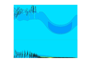
 $\lambda _{v,0}\simeq \lambda _0$ forms. The growth then slows down, and the instability saturates. The distance between the downstream vortices increases. Figure 6 illustrates the instability and the vortex roll-up. The vortex rolls ascend vertically beyond the boundary layer. The vorticity strength reduces with the downstream position. No new instability occurs in bubble two.
Initial instability: growth rate times distance of growth ( $\alpha _i l_0$), distance of growth (
 $l_0/\delta$), wavelength during growth (
 $\lambda _{0}/\delta$), separation length between initial rolls (
 $\lambda _{v,0}/\delta$),
 $Re_{\delta }$,
 $Re_w$ and stratifications 2 and 3 for unstable waves of amplitude
 $a/H=0.30$.

Vertical velocity  $w/c_0$ versus horizontal position, with
 $a/H=0.30$ in Strat.2, where inserts show estimated amplitude of exponential growth (red line): (a)
 $z/H=0.0226$,
 $Re_w=5.9\times 10^4$, run
 $2^*$; (b)
 $z/H=0.00218$,
 $Re_w=5.9\times 10^5$.

Vorticity  $\omega /(c_0/H)$ (colour scale), with
 $a/H=0.30$ in Strat.2: (a)
 $Re_w=5.9\times 10^4$, run
 $2^*$; (b)
 $Re_w=5.9\times 10^5$.

3.5. Bed shear stress
The calculated bed shear stress  $\tau$ is of the form
 $\tau /(\rho c_0^2/2)\simeq A_0\sin [k_{v,0}(x-\hat {x})]$ and oscillates according to the wavenumber
 $k_{v,0}=2{\rm \pi} /\lambda _{v,0}$ of the vortex rolls, where
 $\hat x$ denotes the forward position of the oscillation (figure 7). In the sense of Froude number scaling, the linear long-wave speed is used to scale the stress (e.g. Boegman & Ivey Reference Boegman and Ivey2009; Xu & Stastna Reference Xu and Stastna2020). The stress amplitude is strong in the wave phase and during the vortex roll-up phase, and occurs over a distance of 1–1.5 water depths but is weak otherwise. The maximum strength
 $A_0$ is
 ${\simeq } 1.5\times 10^{-3}$ for the smaller
 $Re_w$, and
 ${\simeq }5\times 10^{-3}$ for the higher
 $Re_w$. The fluctuating stress has a root-mean-square estimate
 $A_0/\sqrt {2}$. The strength and oscillation frequency of the stress both increase when the scale increases. A similar growth of the bed shear stress amplitude with the scale has been found in the case of internal waves of elevation interacting with a weak slope; see Xu & Stastna (Reference Xu and Stastna2020). The
 $Re_w$ value was
 $1.5\unicode{x2013}6\times 10^4$ in their calculations.
Shear stress  $\tau$ (blue line) at the bottom versus horizontal position, with
 $a/H=0.30$, and averaged
 $\tau$ (red line): (a)
 $Re_w=5.9\times 10^4$, Strat.2, run
 $2^*$; (b)
 $Re_w=5.9\times 10^5$, Strat.2; (c)
 $Re_w=6.5\times 10^5$, Strat.3.

3.5.1. Field observations
The bed shear stress has been estimated in field measurements by the Reynolds stress method and the quadratic drag method using acoustic doppler velocimetry. Both methods assume that a log layer exists and extends to the measurement height above the bottom. Measurements on the Australian North West Shelf by Zulberti et al. (Reference Zulberti, Jones and Ivey2020) showed enhanced turbulent shear stress below nonlinear internal solitary waves, and maximum stress 1 Pa. A non-dimensional shear stress becomes 1 Pa/ $(\rho c_0^2/2)\simeq 3 \times 10^{-3}$, where
 $c_0\simeq 0.77$ m s
 $^{-1}$ and
 $Re_w=1.9\times 10^8$ are computed from Zulberti et al. (Reference Zulberti, Jones and Ivey2020). Measurements on the northern shelf of Portugal by Quaresma et al. (Reference Quaresma, Vitorino, Oliveira and da Silva2007) found maximum bed shear stress 0.2 Pa below the strong internal waves. A non-dimensional shear stress becomes 0.2 Pa/
 $(\rho c_0^2/2) \simeq 4 \times 10^{-3}$, where
 $c_0\simeq 0.34$ m s
 $^{-1}$ and
 $Re_w=2\times 10^7$ are calculated from Quaresma et al. (Reference Quaresma, Vitorino, Oliveira and da Silva2007). The strong shear stress measured in the field occurs in the wave phase. The calculated laminar shear stress also occurs below the wave, in the vortex roll-up phase. The relative wave amplitude and pycnocline depth of the field measurements and the model waves are similar (
 $a/H\simeq 0.3$,
 $d/H\simeq 0.2$). The non-dimensional shear stress is also similar.
4. Conclusions
Instability and vortex shedding in the bottom boundary layer beneath internal solitary waves of depression have been calculated by finite-volume code Basilisk in two dimensions. The modelled waves compare very well to exact solutions. The range of the stratification Reynolds number is  $Re_w=c_0H/\nu \sim 1.9\times 10^4\unicode{x2013}6.5\times 10^5$.
Our calculations obtain very accurately the threshold of instability that was measured by Carr et al. (Reference Carr, Davies and Shivaram2008). The very good agreement suggests that the instability in their wave tank experiments was predominantly two-dimensional. The calculated instability is caused spontaneously by the truncation error of the solver. This suggests that small perturbations caused the instability in the wave tank experiments. Note that Sakai et al. (Reference Sakai, Diamessis and Jacobs2020) calculated this kind of instability by large-eddy simulation in three dimensions. They found that the shed vortices were initially two-dimensional.
We have computed the instability threshold and vortex formation for a wider Reynolds number range. The instability is found to depend on the depth of the pycnocline, and has a stronger decay with  $Re_w$ for a deeper pycnocline than for a shallower pycnocline. For example, the threshold amplitude decays according to
 $(Re_w)^{-m_1}$, where
 $m_1=0.23$ when
 $d=0.21H$, and
 $m_1=0.13$ when
 $d=0.16 H$. The instability criterion proposed by Aghsaee et al. (Reference Aghsaee, Boegman, Diamessis and Lamb2012) is re-calculated. Their criterion is not universal and is also very conservative in the sense that only waves of very large amplitude are unstable.
The computations show two separation bubbles. The first is located in the wave phase behind the trough. The second is found well behind the wave phase. The instability emerges as a tiny short-wave disturbance in the back part of bubble one, and moves to the front part when the amplitude increases. Instability and vortex rolls appear in the wave phase behind the trough. No new instability occurs in bubble two.
The vortex formation causes an oscillating bed shear stress. The stress amplitude is strong in the wave phase and during the roll-up phase, and occurs over a distance of 1–1.5 water depths but is weak otherwise. The strong shear stress measured in the field also occurs in the wave phase (Quaresma et al. Reference Quaresma, Vitorino, Oliveira and da Silva2007; Zulberti et al. Reference Zulberti, Jones and Ivey2020). The shear stress computed in the laminar model and measured in the field has similar non-dimensional value (scaled by  $\rho c_0^2/2$) when the non-dimensional amplitude and relative pycnocline depth are similar (
 $a/H\simeq 0.3$,
 $d/H\simeq 0.2$).
Acknowledgements
The critical comments and suggestions by three anonymous referees helped to improve the paper. Professor M.S. Floater is acknowledged for help in improving the language.
Funding
Funding by the Research Council of Norway (Ecopulse, NFR300329) is gratefully acknowledged. The computations were performed on the Norwegian Research and Education Cloud (NREC), using resources provided by the University of Bergen and the University of Oslo (http://www.nrec.no/).
Declaration of interests
The authors report no conflict of interest.


 Open access

