1 Introduction
A frontier goal of laboratory plasma astrophysics is to create the conditions necessary to study the fundamental flow-driven instabilities that give rise to astrophysical dynamos and accretion disk turbulence (Plihon, Bousselin & Palermo Reference Plihon, Bousselin, Palermo, Morales, Bos, Godeferd, Bourgoin, Pinton, Moulin and Aanesland2014; Forest et al. Reference Forest, Flanagan, Brookhart, Clark, Cooper, Desangles, Egedal, Endrizzi, Khalzov and Li2015; Gilmore et al. Reference Gilmore, Lynn, Desjardins, Zhang, Watts, Hsu, Betts, Kelly and Schamiloglu2015; Scime et al. Reference Scime, Keiter, Balkey, Kline, Sun, Keesee, Hardin, Biloiu, Houshmandyar and Chakraborty Thakur2015; Gekelman et al. Reference Gekelman, Pribyl, Lucky, Drandell, Leneman, Maggs, Vincena, Van Compernolle, Tripathi and Morales2016). Generating these instabilities in a laboratory plasma requires sufficient input power and confinement that the resulting plasmas are sufficiently hot to be highly conducting and sufficiently ionised to reduce the role of neutrals in the plasma dynamics (Holland et al. Reference Holland, Yu, James, Nishijima, Shimada, Taheri and Tynan2006; Collins et al. Reference Collins, Katz, Wallace, Jara-Almonte, Reese, Zweibel and Forest2012). These conditions are realised in a large, spherical ring-cusp device referred to as the Big Red Ball (BRB) (Cooper et al. Reference Cooper, Wallace, Brookhart, Clark, Collins, Ding, Flanagan, Khalzov, Li and Milhone2014, Reference Cooper, Weisberg, Khalzov, Milhone, Flanagan, Peterson, Wahl and Forest2016; Weisberg et al. Reference Weisberg, Peterson, Milhone, Endrizzi, Cooper, Désangles, Khalzov, Siller and Forest2017), part of the Wisconsin Plasma Physics Laboratory (WiPPL). This facility has recently demonstrated the ability to produce Helium plasmas with strong neutral depletion in the core.
The depletion of neutrals has been observed in a DC discharge in 1954 by Allen and Thonemann (Allen & Thonemann Reference Allen and Thonemann1954). Many theoretical developments have studied this phenomenon (Fruchtman et al. Reference Fruchtman, Makrinich, Raimbault, Liard, Rax and Chabert2008). However, it has only been measured in inductive discharges. Different techniques such as TALIF (Aanesland et al. Reference Aanesland, Liard, Leray, Jolly and Chabert2007), pressure gages (Gilland, Breun & Hershkowitz Reference Gilland, Breun and Hershkowitz1999) and optical emission spectrometry (OES) (Keesee & Scime Reference Keesee and Scime2006; Boffard et al. Reference Boffard, Jung, Lin and Wendt2009) have been used. This study describes the measurement of neutral helium depletion in DC plasmas using OES. The main diagnostic is a compact, broad-wavelength spectrometer made by OceanOptics. The neutral profiles determined through OES are used in MHD flow simulations to quantify the role of the neutral charge exchange drag forces on the equilibrium ion flow. The obtained velocity profiles are compared with Mach probe measurements.
2 Experimental apparatus
The vacuum vessel is a three metre diameter sphere with 36 axisymmetric rings of permanent magnets forming a multi-dipole ring-cusp for plasma confinement. The magnetic field drops off within 20 cm from the wall resulting in a large unmagnetised bulk (Cooper et al. Reference Cooper, Wallace, Brookhart, Clark, Collins, Ding, Flanagan, Khalzov, Li and Milhone2014). The plasma is produced by an array of 10 lanthanum-hexaboride emissive cathodes inserted into the plasma.
This facility now hosts several plasma experiments which mimic astrophysical phenomena. Two primary goals are to observe the onset of a dynamo effect by an appropriately driven ion flow as well as to study collisionless reconnection. In BRB, the typical achieved velocity is a few kilometres per second. Charge-exchange collisions between ions and neutrals in these plasmas have a non-negligible effect on the flow (Collins et al.
Reference Collins, Katz, Wallace, Jara-Almonte, Reese, Zweibel and Forest2012). Typically, the ion temperature is higher than the neutral gas temperature so after a charge-exchange collision the resulting neutral can leave the plasma at the ion thermal speed, typically within
 $100~\unicode[STIX]{x03BC}\text{s}$
. Although the ion confinement time is approximately 1 ms (Cooper et al.
Reference Cooper, Wallace, Brookhart, Clark, Collins, Ding, Flanagan, Khalzov, Li and Milhone2014, Reference Cooper, Weisberg, Khalzov, Milhone, Flanagan, Peterson, Wahl and Forest2016), the momentum exchange with the neutral gas effectively couples the plasma momentum to the stationary wall (Amnon Fruchtman Reference Amnon2008). The high speeds and shear flow required for creating a dynamo can only be achieved by reducing this neutral drag on the ions.
Each of the ten hot cathodes is powered by a 36 kW power supply. The vessel is equipped with an array of 16 grounded molybdenum anodes fixed in the bulk plasma. The cathodes can be retracted into the cusp in order to apply a torque to the plasma during the discharge (Collins et al.
Reference Collins, Katz, Wallace, Jara-Almonte, Reese, Zweibel and Forest2012; Weisberg et al.
Reference Weisberg, Peterson, Milhone, Endrizzi, Cooper, Désangles, Khalzov, Siller and Forest2017). Gas is injected into the vessel with a piezo-electric puff valve located at the wall of the chamber. The plasma flow is diagnosed by a set of ten Mach probes each equipped with a Langmuir tip to measure the electron temperature. A millimetre-wave interferometer measures the electron density and a Fabry–Pérot interferometer measures the ion temperature. The edge neutral density is measured by two cold cathode gages and a gas residual analyser. A set of two OceanOptics spectrometers are used to analyse the light emitted by the plasma. The spectrometers’ wavelength ranges are 177 to 889 nm and 381 to 512 nm. In this work, we specifically used the smaller range USB4000 spectrometer which provides a measurement of the visible He I emission from
 $n=3\rightarrow 2$
and
 $n=4\rightarrow 2$
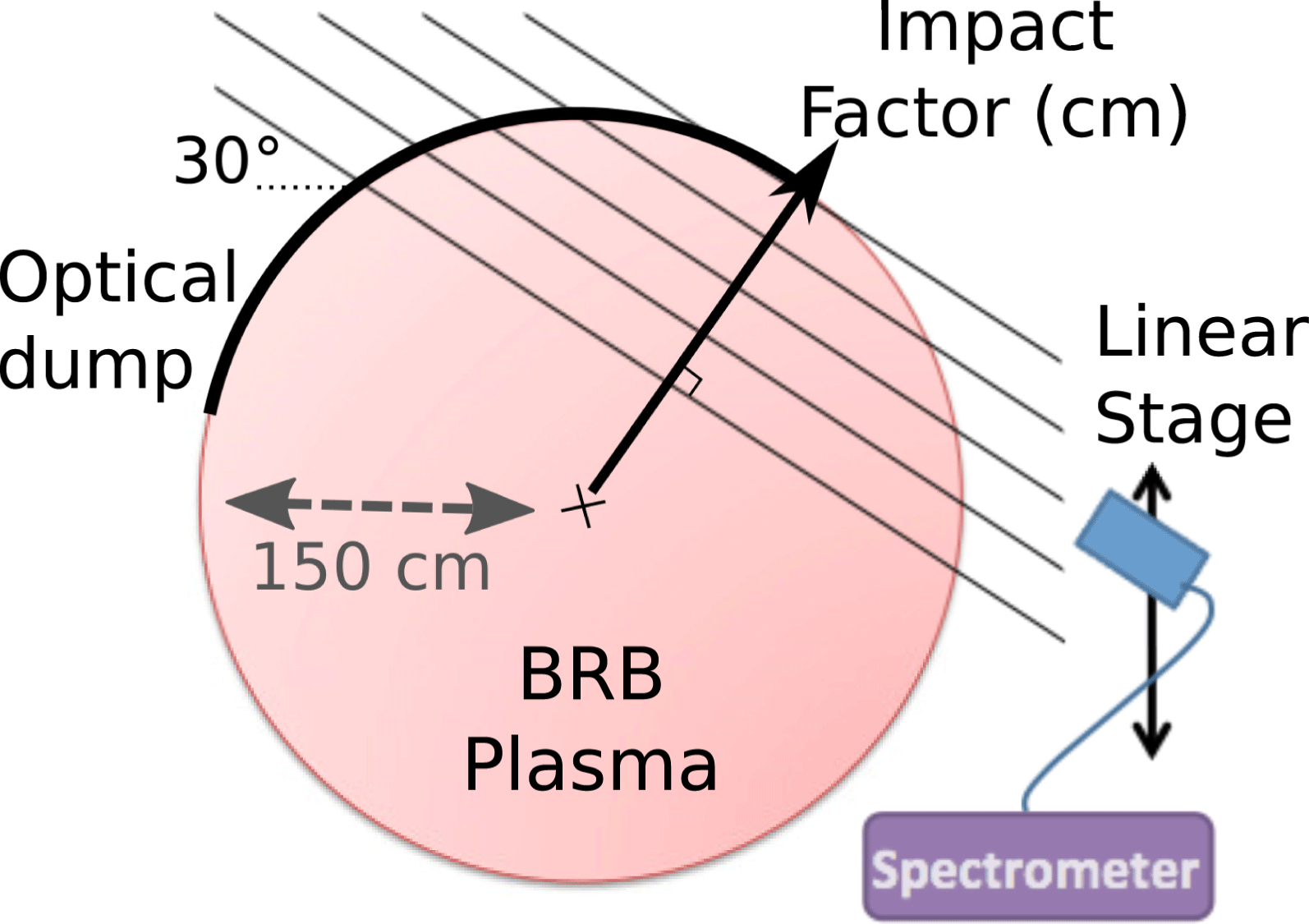
transitions with a typical integration time of 100 ms. A collimator collects the light emitted by the plasma along various chords through the plasma (figure 1). The optical window allows to collect light on chords ranging from 80 cm to 145 cm from the experiment centre. Radiance measurements at various tangency radii are used to infer the emissivity profile for line emission (§ 3). The opposite vessel wall which is in the line of sight of the collimator is equipped with a black optical dump to avoid reflection problems (figure 1).
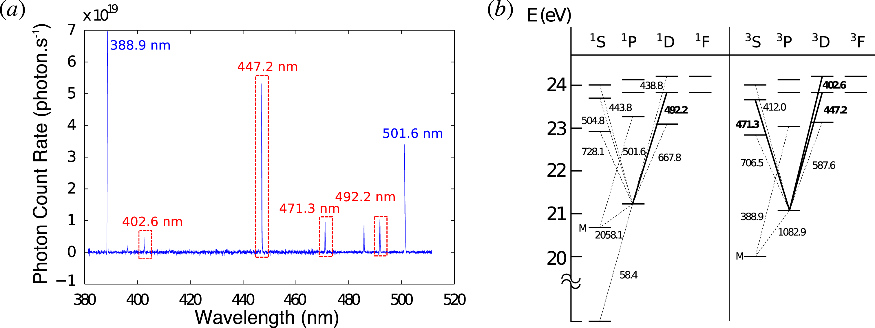
Our analysis focuses on the neutral lines 402.6, 447.2, 471.3 and 492.2 nm which are well resolved by the second spectrometer as seen in figure 2(a) and represented on the Grotrian diagram in figure 2(b).
Schematic of the 1.50 m radius BRB vessel with the spectrometer radiance measurement geometry.

(a) Example measurement of the He I emission spectrum. A radiance calibration is performed to determine the photon flux per spectrometer count rate using a tungsten strip lamp and integrating sphere. (b) Grotrian diagram of neutral helium with the transitions of interest highlighted.

3 Modelling the neutral depletion
3.1 Neutral transport model
The two largest sources of neutrals are gas injection and wall recombination. Relevant processes that act as source and sink terms in the neutral particle continuity equation are direct ionisation by electron-impact collisions, charge-exchange recombination with plasma ions and recombination with free electrons. Neutrals generated by charge-exchange recombination have a long mean free path and are directly lost to the wall.
We assume that the trajectory of neutral particles emanating from the wall are quickly randomised by hard-sphere ion–neutral collisions. Considering the ion–neutral collision frequency (Lieberman & Lichtenberg Reference Lieberman and Lichtenberg2005), effects from both ballistic motion and diffusion are likely important, but we justify this simple diffusion model a posteriori by how well the model fits the measurements (figure 4). Given the source and sink terms discussed above, the neutral continuity equation is
 $$\begin{eqnarray}\displaystyle & \displaystyle \frac{\unicode[STIX]{x2202}N_{n}}{\unicode[STIX]{x2202}t}+\unicode[STIX]{x1D735}\boldsymbol{\cdot }\unicode[STIX]{x1D71E}=S_{\text{recomb}}-S_{\text{ion}}-S_{\text{CX}}, & \displaystyle\end{eqnarray}$$
 $$\begin{eqnarray}\displaystyle & \displaystyle \unicode[STIX]{x1D71E}=-D_{n}\unicode[STIX]{x1D735}N_{n}(r), & \displaystyle\end{eqnarray}$$
 $$\begin{eqnarray}\displaystyle & \displaystyle D_{n}=\frac{V_{th,n}^{2}}{N_{i}\unicode[STIX]{x1D70E}_{HS}V_{th,i}}, & \displaystyle\end{eqnarray}$$
with
 $D_{n}$
the diffusion coefficient of neutrals,
 $\unicode[STIX]{x1D70E}_{HS}$
the cross-section for hard-sphere collisions,
 $V_{th,x}$
the thermal velocity of the species
 $x$
,
 $S_{\text{recomb}}$
the recombination rate per unit of volume,
 $S_{\text{ion}}$
the ionisation rate per unit of volume and
 $S_{\text{CX}}$
is the rate background neutrals are lost to charge-exchange recombination with the ions. These rates can be estimated for typical plasma conditions (Janev et al.
Reference Janev, Langer, Post and Evans1987; Sakabe & Izawa Reference Sakabe and Izawa1991; Huba Reference Huba2013) as
 $$\begin{eqnarray}\displaystyle & \displaystyle S_{\text{recomb}}\approx 10^{12}~\text{cm}^{-3}~\text{s}^{-1} & \displaystyle\end{eqnarray}$$
 $$\begin{eqnarray}\displaystyle & \displaystyle S_{\text{ion}}\approx 10^{15}~\text{cm}^{-3}~\text{s}^{-1} & \displaystyle\end{eqnarray}$$
 $$\begin{eqnarray}\displaystyle & \displaystyle S_{\text{exc}}\approx 10^{15}~\text{cm}^{-3}~\text{s}^{-1}. & \displaystyle\end{eqnarray}$$
These estimates allow us to neglect any volumetric source due to recombination. Note that the charge-exchange collision rate is high and shows the importance of the neutral drag in momentum loss. The ionisation and charge-exchange rates can be written as
 $$\begin{eqnarray}\displaystyle S_{\text{ion}}+S_{\text{CX}}=\langle \unicode[STIX]{x1D70E}v\rangle _{\text{ion}}N_{e}N_{n}+\langle \unicode[STIX]{x1D70E}v\rangle _{\text{CX}}N_{i}N_{n}\approx (\langle \unicode[STIX]{x1D70E}v\rangle _{\text{ion}}+\langle \unicode[STIX]{x1D70E}v\rangle _{\text{CX}})N_{e}N_{n}, & & \displaystyle\end{eqnarray}$$
where we have assumed quasi-neutrality in a single-ion species plasma. Assuming spherical symmetry, the neutrals follow a radial diffusion equation given by:
 $$\begin{eqnarray}\displaystyle r^{2}\left(\frac{\unicode[STIX]{x2202}^{2}N_{n}}{\unicode[STIX]{x2202}r^{2}}-\frac{1}{d^{2}}N_{n}\right)+2r\frac{\unicode[STIX]{x2202}N_{n}}{\unicode[STIX]{x2202}r}=0, & & \displaystyle\end{eqnarray}$$
with
 $d$
the depletion length (Cook et al.
Reference Cook, King, Roberto, Stewart and Yokoyama1984; Yun, Taylor & Tynan Reference Yun, Taylor and Tynan2000; Benilov Reference Benilov2005, Reference Benilov1999),
 $$\begin{eqnarray}\displaystyle d=\sqrt{\frac{D_{n}}{(\langle \unicode[STIX]{x1D70E}v\rangle _{\text{ion}}+\langle \unicode[STIX]{x1D70E}v\rangle _{\text{CX}})N_{e}}}. & & \displaystyle\end{eqnarray}$$
Assuming
 $d$
to be constant in the plasma bulk and the density gradient to be zero in the centre, we have:
 $$\begin{eqnarray}\displaystyle N_{n}(r)=N_{n}(R_{\text{edge}})\times \frac{R_{\text{edge}}}{r}\frac{\sinh \left(\displaystyle \frac{r}{d}\right)}{\sinh \left(\displaystyle \frac{R_{\text{edge}}}{d}\right)}. & & \displaystyle\end{eqnarray}$$
3.2 Neutral particle local emissivity model
The emissivity of a spectral line, defined as the energy emitted by the decay from an excited state
 $i$
to a lower state
 $j$
per unit of volume, per steradian and per second is given by the relation:
 $$\begin{eqnarray}\displaystyle \unicode[STIX]{x1D716}_{ij}=\frac{h\unicode[STIX]{x1D708}_{ij}}{4\unicode[STIX]{x03C0}}N_{i}A_{ij}, & & \displaystyle\end{eqnarray}$$
where
 $h$
is Plank’s constant,
 $\unicode[STIX]{x1D708}_{ij}$
is the frequency of the emitted light,
 $N_{i}$
is the density of the upper state and
 $A_{ij}$
is the Einstein coefficient. Several studies have used a collisional radiative model to measure the electron temperature and electron density of helium plasmas (MacWhirter Reference MacWhirter1965; Sasaki et al.
Reference Sasaki, Takamura, Masuzaki, Watanabe, Kato and Kadota1995; Boivin et al.
Reference Boivin, Loch, Ballance, Branscomb and Pindzola2007; Muñoz Burgos et al.
Reference Muñoz Burgos, Schmitz, Loch and Ballance2012). Commonly used lines include 471.3, 492.2, 504.8, 667.8, 706.5 and 728.1 nm. Their ratio can be written as a function of
 $T_{e}$
and
 $N_{e}$
. Thanks to unmagnetisation, the electron transport is very efficient in the BRB plasma bulk.
 $N_{e}$
and
 $T_{e}$
are constant up to plasma edge where they decrease sharply. Examples of parameters profiles can be seen on Cooper et al. (Reference Cooper, Weisberg, Khalzov, Milhone, Flanagan, Peterson, Wahl and Forest2016) and Weisberg et al. (Reference Weisberg, Peterson, Milhone, Endrizzi, Cooper, Désangles, Khalzov, Siller and Forest2017). As a result, the He line emissivity ratios
 $$\begin{eqnarray}\displaystyle \frac{\unicode[STIX]{x1D716}_{ij}}{\unicode[STIX]{x1D716}_{i^{\prime }j^{\prime }}}=\frac{\unicode[STIX]{x1D708}_{ij}N_{i}A_{ij}}{\unicode[STIX]{x1D708}_{i^{\prime }j^{\prime }}N_{i^{\prime }}A_{i^{\prime }j^{\prime }}}=f(T_{e},N_{e}) & & \displaystyle\end{eqnarray}$$
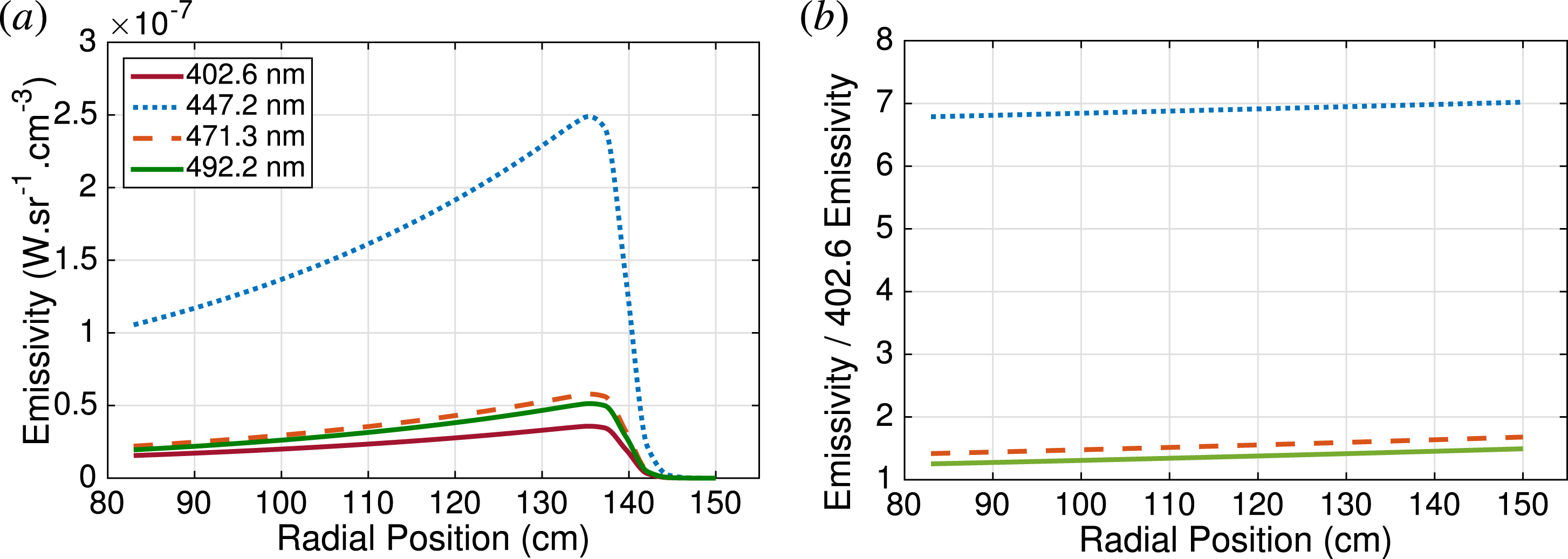
should also be constant. This assumption is verified by measurements shown in figure 3.
(a) Emissivity profiles of each measured line. (b) The emissivity of the lines 447.2, 471.3 and 492.2 is plotted divided by the emissivity of the line 402.6 nm for an 7 eV plasma with a density of
 $7\times 10^{17}~\text{m}^{-3}$
(see run 3 in table 1).

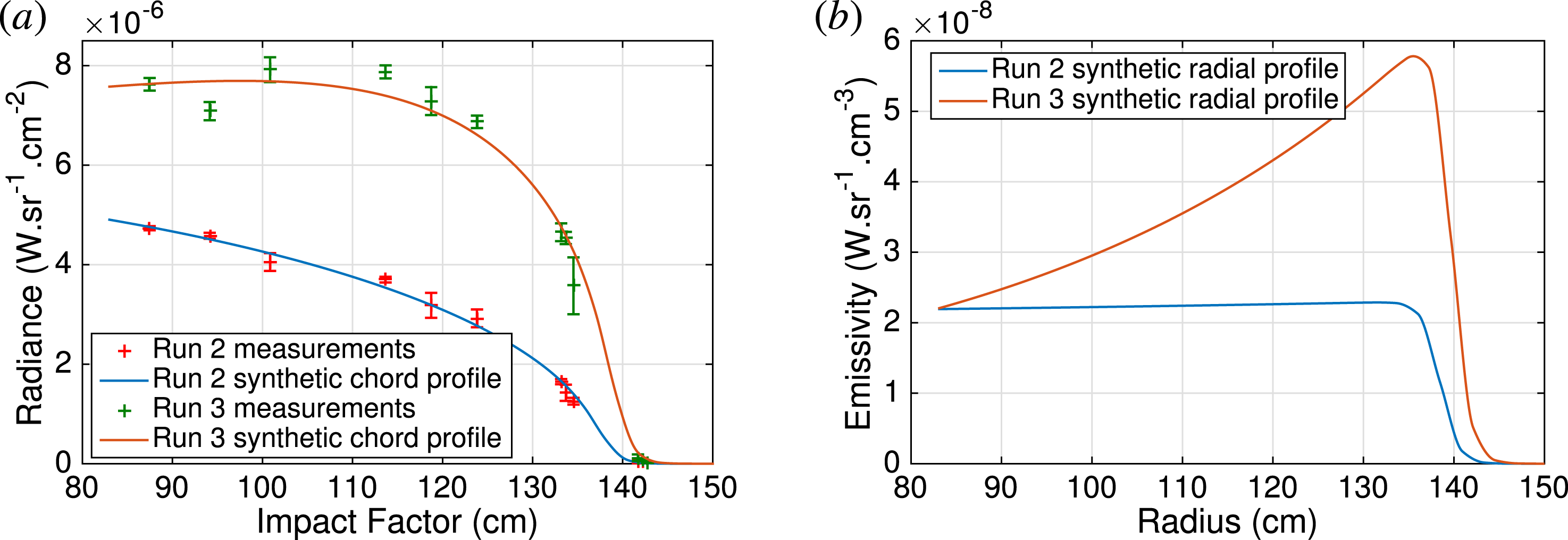
(a) Measurements of the radiance (cross) and fitting routine results in function of the impact factor. (b) Emissivity radial profile corresponding to the inversion of the computed radiant energy profile. Both are for the neutral helium line 471.3 nm, for run 2 and run 3.

Collisional radiative models are used to predict the quasi-steady state populations of the excited states
 $N_{i}$
based on lower state densities
 $N_{k}$
(which include the ground state and metastable states) and plasmas properties such as
 $n_{e}$
and
 $T_{e}$
. The total number density of neutral atoms (
 $N_{n}$
) at a particular location is the sum of the populations of all of the atomic states, but due to the assumption of coronal equilibration this sum is dominated by the sum of the lower states. Therefore,
 $N_{i}\propto \sum _{k}N_{k}\approx N_{n}$
. Equation (3.11) can be rewritten as:
 $$\begin{eqnarray}\displaystyle \unicode[STIX]{x1D716}_{ij}\propto \frac{h\unicode[STIX]{x1D708}_{ij}A_{ij}}{4\unicode[STIX]{x03C0}}N_{n}. & & \displaystyle\end{eqnarray}$$
Combining equations (3.10) and (3.13), the emissivity in the bulk can be expressed as:
 $$\begin{eqnarray}\displaystyle \unicode[STIX]{x1D716}_{ij}(r)\propto \frac{h\unicode[STIX]{x1D708}_{ij}\,A_{ij}}{4\unicode[STIX]{x03C0}}\,N_{n}(R_{\text{edge}})\times \frac{R_{\text{edge}}}{r}\frac{\sinh \left(\displaystyle \frac{r}{d}\right)}{\sinh \left(\displaystyle \frac{R_{\text{edge}}}{d}\right)}. & & \displaystyle\end{eqnarray}$$
The radiant flux from the plasma is collected by a collimating lens which fills a fibre that couples to the spectrometer. Some of the light may be reabsorbed by the plasma due to resonant excitation of the lower states of the observed transitions resulting in a certain amount of dimming of the emission lines. The effect of this reabsorption on the measured radiance is quantified by the optical depth of the plasma
 $\unicode[STIX]{x1D70F}_{ij}$
where the measured radiant flux
 $\unicode[STIX]{x1D6F7}^{\text{meas}}$
is reduced such that
 $\unicode[STIX]{x1D6F7}^{\text{meas}}=\unicode[STIX]{x1D6F7}^{\text{emitted}}\exp (-\unicode[STIX]{x1D70F}_{ij})$
. The optical depth and escape factor can be computed for each transition (MacWhirter Reference MacWhirter1965; Boivin, Kline & Scime Reference Boivin, Kline and Scime2001) and the plasma characteristics.
The obtained mean optical depth is of the order of
 $10^{-7}$
for all observed emission lines and all the light emitted by the plasma comes out of the experiment without being reabsorbed. We will then treat the plasma as optically thin. Measuring the radiance as a function of the impact factor (distance from the line of sight to the centre) we can determine the local emissivity of the plasma by comparing the set of radiance measurements to an Abel transform of our model emission profile as described § 4.1.
4 Measurement of the neutral’s depletion
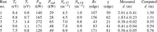
Sections 4.1–4.3 present the results of five OES measurements, the computation of the neutral drag and its effect on the flow in BRB. The plasma parameters corresponding to all these five runs are available in table 1.
Summary of plasma parameters for the different helium OES analysis runs recently made in BRB, the measurement uncertainties are approximately 1 eV on
 $T_{e}$
, 0.15 eV on
 $T_{i}$
,
 $5\times 10^{16}~\text{m}^{-3}$
on
 $N_{e}$
and
 $1\times 10^{17}~\text{m}^{-3}$
on
 $N_{n}$
.
 $N_{e}$
,
 $T_{e}$
and
 $T_{i}$
are measured in the plasma bulk where they are constant.
 $N_{n}$
is measured by pressure gages at the vessel wall. Run 4 has higher uncertainties on the plasma parameters due to a descending trend on
 $N_{e}$
along the run. This trend does not appear on the radiance measurements. Right: summary of the inferred depletion length
 $d$
, given in metres, average on the different lines and its standard deviation for runs recently made in BRB as well as
 $d$
values computed from (3.3) and (3.9) using plasma parameters and tabulated collision rates (Janev et al.
Reference Janev, Langer, Post and Evans1987; Sakabe & Izawa Reference Sakabe and Izawa1991).

4.1 Measurement of the emissivity profiles from the radiant energy
Radiance profiles are measured as a function of the impact parameter by scanning the spectrometer’s collimator on the linear stage. The radiance is a line integrated measurement of the emissivity profile. These experimental measurements are compared to synthetic measurements calculated using a forward model for the emissivity. To compute the synthetic measurements, the edge of the plasma needs to be taken into account. The electron density is empirically modelled by the expression:
 $$\begin{eqnarray}\displaystyle N_{e}(r)=\frac{N_{e0}}{2}[1-\tanh (0.5(r-R_{\text{edge}}))], & & \displaystyle\end{eqnarray}$$
where
 $N_{e0}$
is the electron density measured by the interferometer and
 $R_{\text{edge}}$
is the plasma edge, approximately
 $138~\text{cm}$
. We combine equations (3.14) and (4.1) to include the plasma edge in the expression of the emissivity:
 $$\begin{eqnarray}\displaystyle \unicode[STIX]{x1D716}_{ij}(r)=K[1-\tanh (0.5(r-R_{\text{edge}}))]\frac{\sinh \left(\displaystyle \frac{r}{d}\right)}{\left(\displaystyle \frac{r}{d}\right)}, & & \displaystyle\end{eqnarray}$$
where the amplitude
 $K$
and ionisation length
 $d$
are the fitting parameters of the model. Figure 4 shows the radiant energy measurements and the radiant energy profile computed using equation (4.2) on the top graph and the associated emissivity profile for the neutral helium line 471.3 nm on the bottom one.
4.2 Neutral density profile
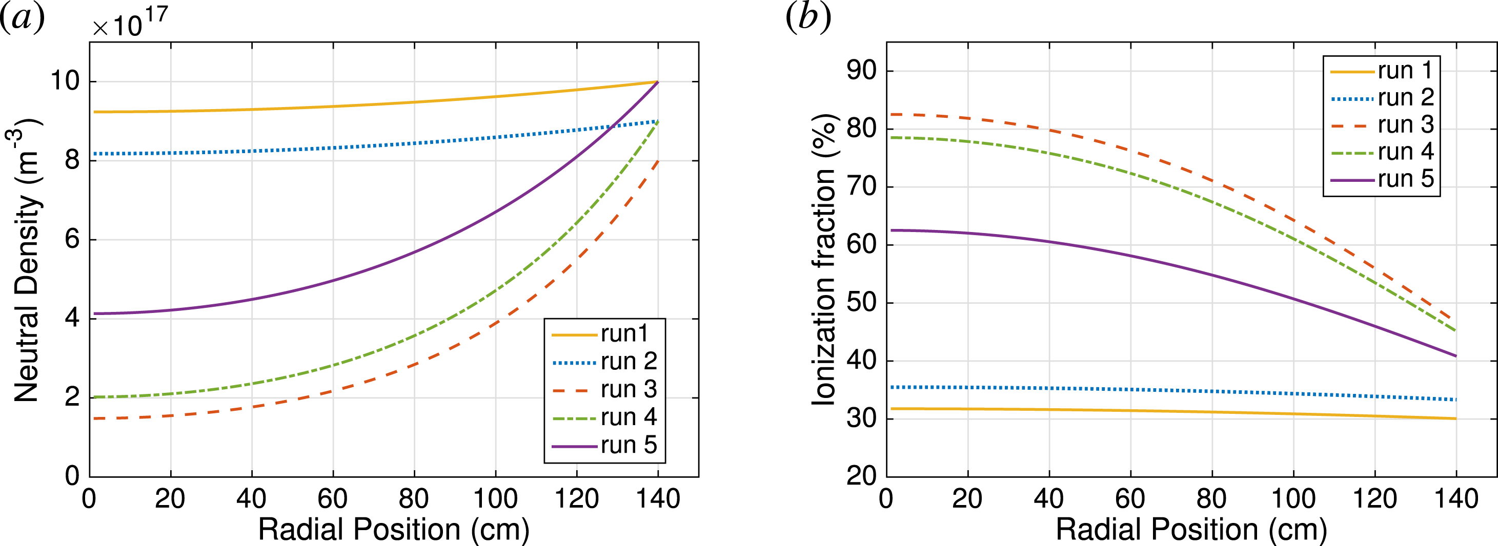
We average the depletion length on the different emission lines in order to obtain one profile of depletion for each run. These results are presented in table 1. The associated emissivity profiles are renormalised to a neutral density profile using the measurements of the pressure at the edge. Neutral density profiles are plotted on figure 5. Different types of density profiles are observed, some with a small depletion in the centre like runs 1 and 2 and others with a bigger depletion of neutrals like runs 3, 4 and 5. The depletion lengths are also computed using (3.3) and (3.9) and tabulated collision rates (Janev et al.
Reference Janev, Langer, Post and Evans1987; Sakabe & Izawa Reference Sakabe and Izawa1991). They are reported in table 1 as well. There is a good agreement between the inferred and the computed depletion lengths, with a maximum of 40 % of relative error between the two values for run 2 and the reproduction of the evolution of
 $d$
for the different runs.
Combining the neutral density profiles with the electron density measurements (table 1), one can compute the ionisation fraction profile (figure 5). The ten lanthanum-hexaboride cathodes and the high confinement time allow high ionisation fraction in the centre of the experiment, up to 80 %.
(a) Inferred neutral density profiles for the different runs. (b) Inferred ionisation fraction profiles for the different runs.

4.3 Evaluation of the neutral drag and flow propagation
In the BRB geometry, the flow is stirred at the edge and propagates inward due to viscosity. The non-flowing neutrals exhibit a drag on the flowing ions via charge exchange. The equation of motion in the plasma can then be written as a classical stationary single fluid Navier–Stokes equation (4.3), where the fluid is the ion population, including a collision term between ions and neutrals which will be called neutral drag.
 $$\begin{eqnarray}\displaystyle Re[(\boldsymbol{v}\boldsymbol{\cdot }\unicode[STIX]{x1D735})\boldsymbol{v}+\unicode[STIX]{x1D735}p]=\unicode[STIX]{x1D6FB}^{2}\boldsymbol{v}-\unicode[STIX]{x1D712}\boldsymbol{v}. & & \displaystyle\end{eqnarray}$$
In this equation,
 $Re$
is the kinetic Reynolds number,
 $\boldsymbol{v}$
is the velocity of the fluid,
 $p$
is the pressure and
 $\unicode[STIX]{x1D712}$
is the neutral drag which can be written as (Huba Reference Huba2013)
 $$\begin{eqnarray}\displaystyle \unicode[STIX]{x1D712}=\frac{L^{2}}{\unicode[STIX]{x1D708}_{\text{visc}}\unicode[STIX]{x1D70F}_{in}}=38.2\frac{(n_{0}n_{i})_{18}Z^{3}L_{m}^{2}}{T_{i,eV}^{2}}. & & \displaystyle\end{eqnarray}$$
Here,
 $\unicode[STIX]{x1D70F}_{in}$
is the ion–neutral collision time and
 $\unicode[STIX]{x1D708}_{\text{visc}}$
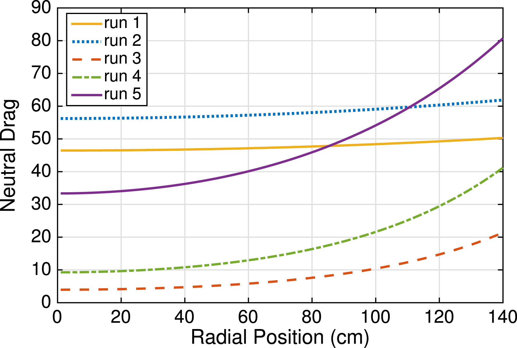
is the Braginskii viscosity. From the neutral density profiles (figure 5), one can compute the neutral drag in function of the radial position using (4.4) (figure 6). It is interesting to notice that even though the neutral density is lower for run 5 than for runs 1 and 2, the neutral drag for these runs is comparable due to the differences in ion temperatures.

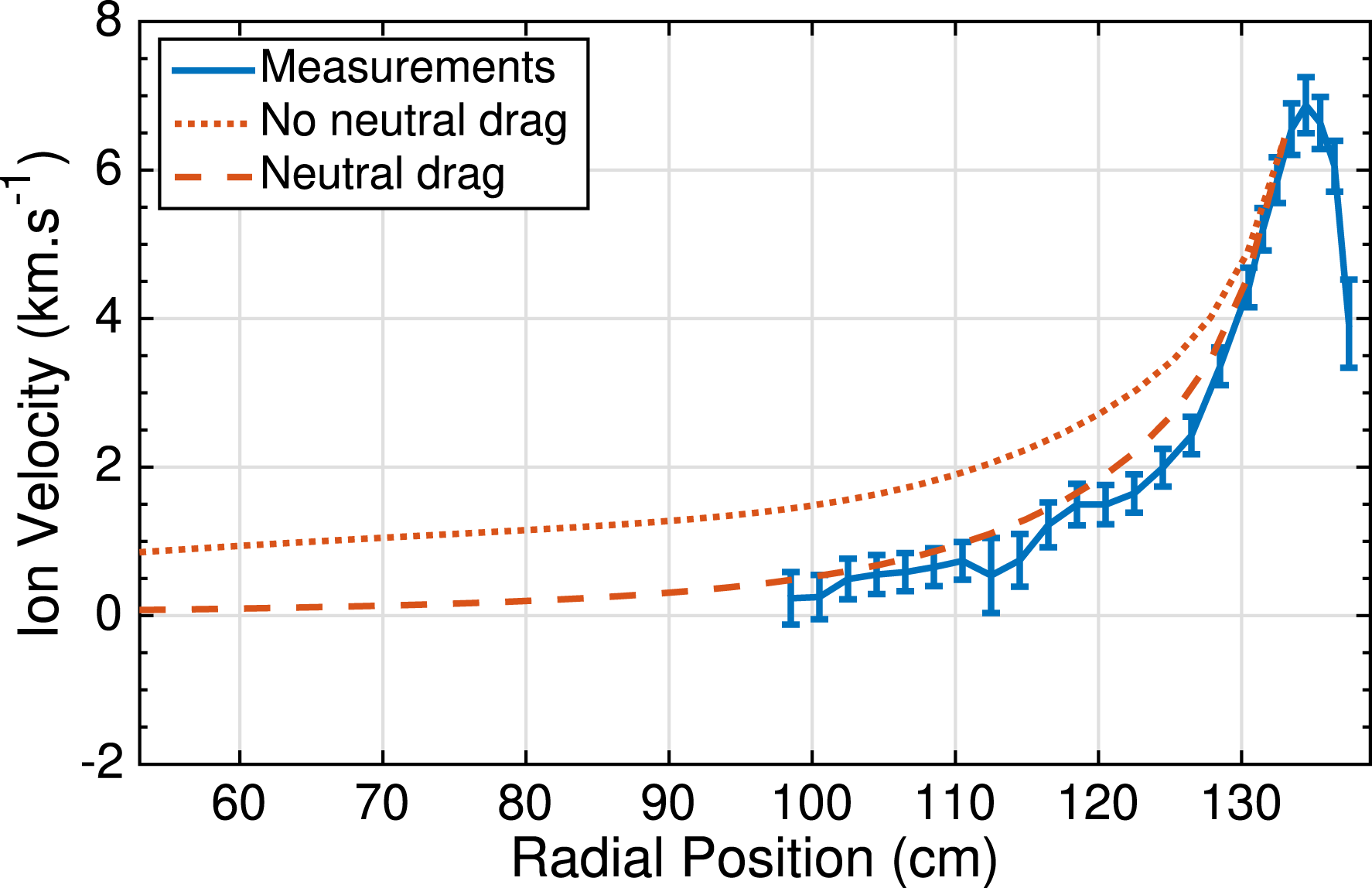
A single fluid simulation code has been previously developed by Khalzov et al. (Reference Khalzov, Brown, Cooper, Weisberg and Forest2012), Khalzov, Cooper & Forest (Reference Khalzov, Cooper and Forest2013) to simulate the flow and the dynamo onset in the BRB vessel. The neutral drag has been implemented into this code to evaluate its influence on the flow. As velocity measurements had not been made for the runs of interest, we used Mach probe velocity measurements of another run to fix the boundary condition and to compare results of the simulation with measured flow. The simulation has been made with a boundary condition of
 $6.5~\text{km}~\text{s}^{-1}$
at 134 cm from the centre, with and without neutral drag, for the values of the neutral drag and Reynolds number of the different runs.
The velocity computed with the neutral drag decreases faster than the velocity computed with no neutral drag and better match the measured velocity profiles. This agreement is verified for every obtained value of the drag. It demonstrates that the neutral drag plays an important role in the ion dynamics. The difference in velocity profiles without any drag is due to the specific Reynolds number of each run. This difference is small compared to the effects of the neutral drag. A low neutral drag significantly helps to viscously couple the edge torque across the plasma.
Khalzov et al. (Reference Khalzov, Brown, Cooper, Weisberg and Forest2012, Reference Khalzov, Cooper and Forest2013) have also studied the impact of the geometry of the flow drive on the onset of an MHD instability in BRB. They have shown that an optimised flow can produce a growing MHD mode for a moderate
 $Re=150$
and Rm ranging between two critical values. Using their drive geometry, one can study the impact of neutral drag on the MHD stability. Without neutral drag, the flow resulting from the applied torques should produce an instability as predicted by Khalzov et al. (Reference Khalzov, Brown, Cooper, Weisberg and Forest2012, Reference Khalzov, Cooper and Forest2013). With a uniform neutral density profile, the resulting charge-exchange drag slows the flow enough to stabilise this MHD instability. Accounting for the hollow neutral profile due to the neutral dynamics, the flow is slightly less damped illustrating the importance of quantifying neutral dynamics in these plasmas.
Typical measured velocity profile and simulated velocity profile of the plasma for run 3 with and without the neutral drag taking into account in the simulations.

5 Conclusion and further work
The use of neutral helium radiance measurements, coupled with a model for the diffusion and the electron-impact excitation of neutral atoms, allows us to measure the depletion of neutrals within plasmas in the BRB. Various profiles of neutral density have been observed from flat to very hollow. The measured neutral density profiles provide a means of quantifying the neutral drag in flowing plasmas. Increasing the neutral depletion lowers the drag and allows a better coupling of torques applied to the edge of the plasma to drive flows throughout the plasma. Modelling the neutral burnout correctly is important to predict the flow geometry and the MHD stability of the plasma. The ion temperature and the ionisation fraction must be increased to decrease the neutral drag. This can be done using Electron Cyclotron Heating (ECH) power, currently under development in BRB. Finally, the derived diffusion model is sufficient to predict the neutral density profile shape, but the current set of measurements is insufficient to adequately test whether other effects are important in characterising the neutral dynamics. Further work on addressing ballistic transport, the presence of other neutral components, and measurements of the neutral temperature are in development.
Acknowledgements
This work was funded in part by NSF award no. PHY 0923258, ARRA MRI, NSF award no. PHY 0821899, Center for Magnetic Self Organization in Laboratory and Astrophysical Plasmas, and DOE award no. DE-SC0008709, Experimental Studies of Plasma Dynamos. C.C. acknowledges support by the ORISE Fusion Energy Sciences Graduate Fellowship. V.D. was supported by CNRS PICS contract PlasmaDynamo and by French National Research Agency under contract ANR-13-JS04-0003-01