1. Introduction
Turbulence in the troposphere is created in shear flows which emanate from meteorologic processes such as vertical thermal convection due to solar heating, wind deflection over large objects, so-called orographic interference, and wind shear at inversion layers. While the first two mechanisms are frequently found in the lowest layer of the atmosphere, i.e. the atmospheric boundary layer reaching altitudes between 1 and 3 km, the latter mechanism may also be found at high altitudes, even above the troposphere (Wyngaard Reference Wyngaard1992). Turbulence in the atmosphere is produced by the formation of large eddies with length scales three to four orders of magnitude larger than the chord length of aircraft (Stull Reference Stull1988). These eddies decay continuously into smaller eddies. Within a certain range of eddy sizes, the inertial subrange, the transfer of turbulent kinetic energy to smaller eddies is described by the power-law behaviour (
 $-5/3$
-law) postulated by Kolmogorov (Reference Kolmogorov1941) (see also Pope Reference Pope2000). Only for very small length scales of the order of millimetres the kinetic energy is eventually dissipated by molecular friction. For aircraft flying through turbulence this implies unsteady oncoming flow of varying direction and magnitude due to the superposition of eddies of different sizes (MacCready Reference MacCready1962). Natural laminar flow (NLF) aerofoils may be particularly affected by such disturbances since their goal of maximising the laminar portion of the wing boundary layer in order to save drag can be corrupted by the enhanced excitation of boundary-layer disturbances through increased small-scale turbulence levels. Compared with calm flight conditions, higher levels of atmospheric turbulence may create stronger boundary-layer disturbances, which subsequently amplify according to the stability properties of the boundary layer and trigger premature transition (Nishioka & Morkovin Reference Nishioka and Morkovin1986; Crouch Reference Crouch1992a
; Kachanov Reference Kachanov2000; Saric, Reed & Kerschen Reference Saric, Reed and Kerschen2002; Herr Reference Herr2003). However, there is little knowledge of whether the smaller scales of atmospheric turbulence resonate efficiently with the natural modes of the boundary layer through the receptivity process. Furthermore, as a consequence of the
 $-5/3$
law, the kinetic energy of turbulence changes proportionally on all flight-relevant length scales for varying atmospheric conditions. Under moderately turbulent conditions the amplitudes inherent to turbulent flow fluctuations with length scales of the order of the chord length can lead to time-dependent and unsteady aerofoil effects (McCroskey Reference McCroskey1982; Bisplinghoff, Holt & Halfman Reference Bisplinghoff, Holt and Halfman1996; Fung Reference Fung2008; Reeh, Weismüller & Tropea Reference Reeh, Weismüller and Tropea2014). Numerous studies have been conducted in order to investigate both effects, receptivity to small-scale turbulence and time-dependent changes of the outer flow, separately in wind tunnels (Schubauer & Skramstad Reference Schubauer and Skramstad1948; Kendall Reference Kendall1984, Reference Kendall1998; Dietz Reference Dietz1999; Mish & Devenport Reference Mish and Devenport2003; Fransson, Matsubara & Alfredsson Reference Fransson, Matsubara and Alfredsson2005; Studer et al.
Reference Studer, Arnal, Houdeville, Seraudie and Govindarajan2006; Kenchi, Matsubara & Toshihiko Reference Kenchi, Matsubara and Toshihiko2008; Matsubara, Takaichi & Kenchi Reference Matsubara, Takaichi and Kenchi2010) or in numerical simulations (Cebeci, Carr & Jang Reference Cebeci, Carr and Jang1989; Herbert, Stuckert & Esfahian Reference Herbert, Stuckert and Esfahian1993; Bertolotti Reference Bertolotti1997, Reference Bertolotti1999; Schrader et al.
Reference Schrader, Brandt, Mavriplis and Henningson2010; Yeo et al.
Reference Yeo, Zhao, Wang and Ng2010). However, due to the specific composition of atmospheric turbulence, all of the effects acting on an aircraft wing cannot be simulated simultaneously, neither in generic experiments nor in elaborate computations.
Previous in-flight studies concentrated either on the characterisation of the free-stream turbulence, e.g. MacCready (Reference MacCready1962) and Riedel & Sitzmann (Reference Riedel and Sitzmann1998), or investigated boundary-layer transition under perfectly calm conditions, e.g. Erb (Reference Erb2002) and Peltzer (Reference Peltzer2008). Runyan & George-Falvy (Reference Runyan and George-Falvy1979) and Horstmann, Quast & Redeker (Reference Horstmann, Quast and Redeker1989) compared transition positions measured in flight experiments and in a low-turbulence wind tunnel with
 $N$
-factor curves obtained with linear stability analysis. Seitz & Horstmann (Reference Seitz, Horstmann, Meier and Sreenivasan2006) investigated the frequency content and spanwise extent of Tollmien–Schlichting (TS) wavepackets on a wing boundary layer in flight under calm atmospheric conditions. Zanin (Reference Zanin1985, Reference Zanin1989, Reference Zanin2008) reported some comparisons between free-stream turbulence and boundary-layer instabilities. In this work the participation of TS wavepackets in the transition process was observed for all oncoming flow conditions, even when flying through clouds with significantly elevated turbulence intensities. However, this investigation was limited by the available instrumentation and by inevitable inviscid aerofoil effects, i.e. variations of the pressure gradient due to the time-varying oncoming flow, which were not considered. Carpenter, Saric & Reed (Reference Carpenter, Saric, Reed, Schlatter and Henningson2010) and Saric, Carpenter & Reed (Reference Saric, Carpenter and Reed2011) conducted in-flight receptivity studies for swept wings but their results cannot be transferred to the case of two-dimensional boundary layers. A comprehensive measuring platform for the investigation of the effect of atmospheric turbulence on a straight wing airplane has been developed by Weismüller (Reference Weismüller2011). His results concentrated on gliding flights through turbulence at high angles of attack. Reeh et al. (Reference Reeh, Weismüller and Tropea2014) presented in-flight results for low angles of attack in moderately turbulent conditions obtained with the same research aircraft, including a detailed transition investigation with wall-microphones on the lower side of a NLF aerofoil. The appearance of TS wavepacket without pronounced discrete frequencies was confirmed in flight experiments under moderately turbulent conditions. Transition fluctuations were related to angle-of-attack variations.
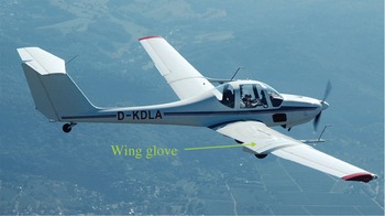
The G109b research aircraft.

The present work is devoted to the investigation of the influence of atmospheric turbulence on the flight performance at low lift coefficients with the ambition of considering all important aerodynamic effects occurring on a two-dimensional NLF wing section in cruising flight. In order to assess the problem, flights through turbulent atmospheric conditions are compared with reference flights through calm conditions. The importance of the time dependence of viscous airfoil effects in the presence of typical turbulence levels is addressed, emphasising the boundary-layer development on a NLF aerofoil. In particular, the question whether there is any sign of bypass transition and the role of TS waves in the presence of typical atmospheric turbulence conditions are investigated.
2. Experimental set-up
A comprehensive description of the research aircraft is provided in previous studies by Weismüller (Reference Weismüller2011) and Reeh, Weismüller & Tropea (Reference Reeh, Weismüller and Tropea2013a ). Only a short summary of the existing system will be given here. Since certain measurement equipment has been substantially modified, these new subsystems will be described in more detail.
2.1. Test aircraft and NLF wing glove
The test aircraft shown in figure 1 is a Grob G109b motorised glider sufficiently powered to achieve viable climb rates for the experiments while carrying fuel, the measurement equipment and a crew of two, the pilot and the flight test engineer. The testbed for the actual aerodynamic experiments is a wing glove mantling the original wing in the section between the airbrake and the aileron of the right-hand wing. The wing glove is rectangular in cross-section, yielding approximately two-dimensional flow in its centre section, which has been verified by CFD computations (maximum cross-flow components below 2 % for angles of attack below
 $6^{\circ }$
). It is based on a NLF aerofoil typical for sailplane applications. The profile has been modified by Weismüller (Reference Weismüller2011) to compensate for the asymmetric aircraft configuration and to offer an advantageous pressure distribution for the transition investigations. Characteristic aerofoil geometry data for the wing glove and the aircraft wing can be found in table 1.
Aerofoil geometry parameters normalised by the chord length.

2.2. Measuring instrumentation, data acquisition and system synchronisation
The reference data is obtained from an air data system consisting of sensors for the static (Setra 270) and the dynamic pressure (Setra 239HP), the temperature (PT 1000) and the relative humidity (Hygrosens CON-Hytemod-I2C). Furthermore, a wind vane captures the reference angle of attack and the side-slip angle with an accuracy of
 $0.1^{\circ }$
. The air data system for the reference values is unchanged compared with the investigations of Weismüller (Reference Weismüller2011) and Reeh, Weismüller & Tropea (Reference Reeh, Weismüller and Tropea2013b
). A systematic estimation of the experimental uncertainty yields a maximum error for the true airspeed of 0.9 % and 1.5 % for the determination of the chord Reynolds number
 $\mathit{Re}$
.
For the present research objectives the existing instrumentation has been successively changed, improved and extended beyond the set-ups reported by Erb (Reference Erb2002), Weismüller (Reference Weismüller2011) and Reeh et al. (Reference Reeh, Weismüller and Tropea2013a ). The most important components of the system and their relevance for the investigation are described in the following.
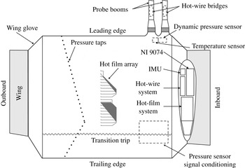
Sketch of the lower side of the wing glove.

The high-frequency content of the oncoming flow is important for the excitation of boundary-layer instabilities, i.e. the initial amplitudes of the oncoming flow disturbances may determine the course of boundary-layer transition. In order to gain insight into the spectral composition of atmospheric turbulence, frequencies of several kilohertz need to be resolved with high sensitivity. Furthermore, a valuable contribution to atmospheric research can be achieved by resolving the dissipative range of the kinetic energy density spectrum of the turbulence. Therefore, the free-stream turbulence is measured with two X-hotwire probes, enabling the measurement of velocity fluctuations in all three spatial directions and the two flow angles. The investigation of the energy density spectrum of atmospheric turbulence requires ultra-low noise anemometers, a sophisticated signal conditioning and high sampling frequencies. Thus, a hotwire diameter of only
 $2.5~{\rm\mu}\text{m}$
is used in order to reduce the thermal inertia of the sensors. The entire system has been specifically configured and designed for such probes. A custom four-channel constant temperature anemometer (CTA) system is used. The measuring bridge circuits and the feedback controllers are installed directly in the two booms pointing into the free stream, reducing probe cable length to a minimum (
 ${<}0.8~\text{m}$
). The signal conditioning unit is installed in the storage pod attached to the wing glove. The anemometers are battery supplied to avoid high-frequency disturbances from DC/DC-converters. Signals are conditioned in two parts, a DC and an AC coupling. While the DC part with a pass bandwidth of 3 kHz (sampling frequency 16 kHz) allows correlations of the oncoming flow quantities with other flow quantities and the motion of the wing glove, the AC part is coupled with a band-pass filter (edge frequencies 50 Hz and 8 kHz) and a low noise amplifier (amplification between 200 and 1000) to detect the dissipation range in the atmospheric turbulence spectra. A Delta-Sigma A/D-converter (logging data rate 25 kHz) is used to avoid aliasing of the well-known self-induced electronic anemometer noise at high frequencies (Freymuth & Fingerson Reference Freymuth and Fingerson1997). The X-wires are calibrated before each flight with effective angle scheme from Bradshaw (Reference Bradshaw1971), which is also described by Reeh et al. (Reference Reeh, Weismüller and Tropea2014).
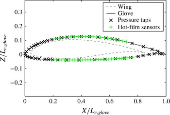
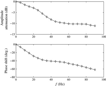
The instantaneous pressure distribution on the wing section is important for the evaluation of aerofoil lift and the investigation of unsteady flow phenomena. Furthermore, it is a prerequisite for boundary-layer transition investigations to measure the pressure distribution accurately to provide smooth boundary conditions for the accompanying numerical computations. The pressure distribution is recorded with 48 Sensortechnics HCL-12X5P miniature pressure transducers installed beneath the surface of the wing glove (static accuracy better than 3.2 Pa). The distribution of the sensors on the wing section is shown in figures 2 and 3. Due to the short tubes (lengths less than 0.1 m) connecting the pressure taps to the transducers, fast pressure changes resulting from turbulent gusts can be detected. However, even the short pressure lines affect the frequency response considerably, as can be seen in figure 5. In order to measure accurately with a bandwidth of at least 45 Hz, a dynamic in situ calibration (Perls, Miles & Wilner Reference Perls, Miles and Wilner1960; Damion Reference Damion1994; ISA 2002) was carried out and the pressure measurements are corrected in a forward–backward Fourier transformation in the postprocessing of the experimental data yielding a dynamic error of less than 3 % for a 90 Hz bandwidth. Therefore, a device generating sinusoidal pressure signals in steps of 5 Hz was connected to each pressure tap (opening diameter 0.3 mm) up to frequencies of 90 Hz. The same signal was also applied to a calibration tap feeding a Kulite XCQ-93 reference sensor. The reference sensor has a high accuracy, very flat frequency response far beyond the targeted frequency and it was directly connected to a calibration reference tap without a pressure line, i.e. with minimum dead volume. The obtained amplitude and phase difference between each sensor of the wing glove pressure system and the reference sensor is used to correct the pressure measurements. The frequency response function
 $H_{rs}$
(Mish & Devenport Reference Mish and Devenport2003; Bendat & Piersol Reference Bendat and Piersol2010) is determined by the dimensionless ratio between the cross-spectral density
 $G_{s,r}(f)$
of the sensor (subscript
 $s$
) and the reference sensor (subscript
 $r$
) and the auto-spectral density
 $G_{r,r}(f)$
of the reference sensor
 $$\begin{eqnarray}H_{s,r}(f)=\frac{G_{s,r}(f)}{G_{r,r}(f)}=\frac{E\left[P_{s}(f)\cdot P_{r}^{\ast }(f)\right]}{E\left[P_{r}(f)\cdot P_{r}^{\ast }(f)\right]},\end{eqnarray}$$
where
 $f$
is the frequency,
 $P_{s}$
is the complex Fourier coefficient of the sensor signal and
 $P_{r}$
is the coefficient of the reference sensor. Here
 $E[\,]$
is the expectation and the asterisk denotes the complex conjugate. The pressure signal
 $p_{cor}$
is corrected by multiplying the Fourier transform of the measured signal
 $P_{m}$
with the reciprocal of the transfer function
 $H_{s,r}$
and applying the inverse Fourier transform
 ${\mathcal{F}}^{-1}$
:
 $$\begin{eqnarray}\displaystyle p_{cor}(t) & = & \displaystyle {\mathcal{F}}^{-1}\{P_{cor}(f)\}\nonumber\\ \displaystyle & = & \displaystyle {\mathcal{F}}^{-1}\left\{P_{m}(f)\frac{1}{H_{s,r}(f)}\right\}\nonumber\\ \displaystyle & = & \displaystyle {\mathcal{F}}^{-1}\left\{\frac{|P_{m}(f)|}{|H_{s,r}(f)|}\exp [-\text{i}\arg (H_{s,r}(f))]\right\}.\end{eqnarray}$$
Sensor distribution on the wing section.

The question whether the aerodynamic forces directly translate into motions of the aerofoil and whether the elasticity of the wing plays an important role in the process can be partially answered by the integration of two inertial measurement units (IMUs) into the research aircraft. A SBG Systems I500A attitude and heading reference systems (AHRS) is included in the wing glove structure and an IG-500N inertial navigation system (INS) is installed in the fuselage of the aircraft in proximity to its center of gravity. Both systems include three accelerometers (accuracy 0.5 mg) and three gyros (accuracy
 $0.5^{\circ }$
at
 $300^{\circ }~\text{s}^{-1}$
), providing information on the actual accelerations and angular velocities of the aerofoil and the fuselage at an output rate of 100 Hz. Of particular interest is the minimum magnitude of oncoming flow disturbances that leads to a motion of the wing section and at larger oncoming flow disturbance levels, the response of the airframe to unsteady aerodynamic behaviour. The integration of the difference in acceleration and angular velocities yields the relative motion between the two IMUs.
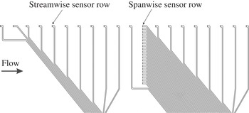
The hot-film sensor array.

Boundary-layer transition is investigated with a 64-channel constant temperature hot-film system. This very compact device has been specifically configured and custom designed for in-flight experiments. It fits in the small storage pod attached to the wing glove, resulting in very short cable lengths to the sensors (
 ${\approx}1.3~\text{m}$
only). Several other features have been included to obtain high signal-to-noise ratios. Using FPGA technology, the hot-film system operates with an internal sampling frequency of 400 kHz per channel. A real-time moving average enables a 25-fold oversampling of the signals and provides an output data rate of 16 kHz for logging. Depending on the measurement task a DC- or an AC-coupling of the amplified signal can be acquired. For boundary-layer instability studies the utilisation of the full measurement range in the AC-mode is especially convenient. Customised arrays of Senflex hot films are used for the experiments. The arrays are manufactured such that the hot-film sensors and the leads shown in figure 4 are deposited on a polyimide substrate, leading to a maximum thickness of
 $8~{\rm\mu}\text{m}$
, which is below the relevant level for vortex receptivity in the present case, estimated with the equations and results provided by Dietz (Reference Dietz1999). The array sheets bonded onto the wing section have a thickness of
 $51~{\rm\mu}\text{m}$
. Filler has been carefully applied at the upstream edges to provide a smooth and flush ramp to the array. Seitz (Reference Seitz2007) shows that such a slight change of the aerofoil contour is insignificant for the pressure distribution; hence, also for the boundary-layer development. An array comprises a hot-film sensor row in the streamwise direction (sensors equidistantly distributed every 28 mm) and a spanwise sensor row consisting of 21 elements in an equidistance of 5 mm. While the streamwise row captures the instability amplification, the streamwise changes in the transition process and the breakdown to the turbulent boundary layer, the spanwise row detects the spanwise bandwidth of the TS wavepackets, i.e. the spanwise distribution of the waves. On the upper side of the wing glove a mirrored version of the array on the lower side is positioned such that the spanwise row lies within the growth region of TS wavepackets for the investigated flight cases. The dynamic sensor response is matched by tripping the boundary layer close to the leading edge in a calibration flight. The resulting turbulent boundary layer disturbance spectrum best resembles a white noise source for an in situ matching of the whole array. However, the slight weakening of the fluctuation intensity in the streamwise direction in a fully turbulent boundary layer is not accounted for. It will be seen in § 3.2 that this effect is insignificant for the interpretation of the results of the present investigation.
Typical Bode diagram for a pressure sensor connected to the pressure tap by a 0.15 m long pressure line.

All measuring system components are triggered with the edges of TTL signals provided by a National Instruments cRIO 9074 system.
3. Results
3.1. Flight test programme
The flight test programme consisted of 11 days of flying in September and October 2013 in which the complete experimental set-up described in § 2.1 was available. A flight comprised one or two straight glides from a pressure altitude of almost 3300 m to approximately 650 m in which data was collected over up to 14 intervals of 20 s. The engine was shut off to avoid unwanted interferences with the flow and the measurement instrumentation. Before and after each flight a photo of the leading edge of the wing glove was taken in order to exclude any experimental data where bug strikes may have affected the transition results. For the definition of the flow on the wing glove, the angle-of-attack and the side-slip-angle information from a wind vane instrument was low-pass filtered and indicated to the pilot in a special command display to enable a predefined flight condition to be maintained. Atmospheric turbulence inevitably demands control inputs of the pilot in order to maintain a specific flight condition. However, pilots naturally only respond to larger excursions caused by the oncoming flow disturbances; hence the pilot acts as a high-pass filter. In the present experiments the flow angles were displayed to the pilot employing a low-pass filter in order to avoid unnatural control inputs. While long-wave deviations from the targeted flow angles could be compensated, the effect of inevitable and uncontrollable small gusts was intentionally present. The procedure best resembled a cruising flight situation with emphasis on the particular flow state on the wing glove.
Atmospheric turbulence was mainly encountered due to thermal convection, but orographic wind interference from a mountain ridge close to the airfield was also a possible and predictable source of turbulence. Although the experiments took place in the late season of the year and thermals were not as intense as in summer, considerable turbulence was still encountered. However, this work only investigates the influences of moderate turbulence on the NLF wing section. Moderately turbulent conditions are found throughout most of the year and they occur frequently in between local zones of strong turbulence, e.g. in strong thermals. These conditions are therefore of primary interest for aerofoil designers regarding efficiency improvements.
3.2. Transition development for calm atmospheric conditions
Approximately half of the flight measurements stated above were conducted to verify the steady flow behaviour. The observations of Reeh et al. (Reference Reeh, Weismüller and Tropea2014) made with a low-cost wall microphone transition detection system on the same wing glove served as a reference to determine whether the hot-film array foil had an influence on boundary-layer receptivity and transition. For the transition investigation 60 hot films were used on both sides of the wing section: 40 hot films were distributed on the lower side of the aerofoil, using 20 sensors in a streamwise row and 21 in a spanwise sensor row including one overlapping sensor element as depicted in figure 4. The remaining 20 sensors were aligned in a streamwise row on the upper side for simultaneous transition investigations. Calm atmospheric conditions, as can be found early in the morning and in high altitudes, allow for very precise flying with an angle of attack variation below
 $0.1^{\circ }$
. The velocity may vary slightly (
 ${<}2\,\%$
) due to the phugoid motion of the aircraft and the air properties change slowly while descending. Nevertheless, the changes with altitude are insignificant over the measurement interval of 20 s. The Reynolds number variation remains within less than 2 %. Therefore, time-averaged transition data can be obtained with high precision, but the exact reproducibility of the Reynolds number is complicated due to the meteorologic variations from flight to flight and weight differences of the aircraft, depending on the fuel level.
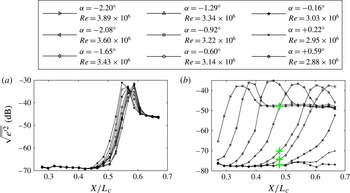
In order to understand the behaviour of NLF aerofoils in flight through atmospheric turbulence, it is necessary to examine the steady angle-of-attack dependency of transition experimentally. The angle of attack determines the pressure distribution and thereby the steady-state development of the boundary layer on the wing glove. Figure 6 demonstrates the transition process on both sides of the wing section by means of the root-mean-square (RMS) voltage fluctuations
 $\sqrt{\overline{e^{\prime 2}}}$
in the streamwise direction obtained by the constant-temperature hot-film system. Hot-film signals can be related to the wall-shear stress fluctuations by a specific cooling law, see Seitz (Reference Seitz2007), but for the present investigation of the transition behaviour the voltage RMS values are sufficient. It should be noted that the nonlinear sensor characteristic of surface hot films does not allow for direct comparisons between the obtained voltage values and theoretical disturbance amplitudes. Nevertheless, the unambiguous qualitative shape of the RMS curves offers sufficient information for the present investigation. The logarithmic presentation in decibels highlights calibration differences between the sensors and reflects the signal-to-noise ratio. In general, very good matching of the sensors can be inferred from the smooth evolution of the curves.
Transition development on both sides of the wing glove under calm flight conditions. The larger
 $+$
marker symbols on the lower side will be referred to in § 3.2.2: (a) upper side; (b) lower side.

All of the information shown in figure 6 were obtained in a single gliding flight and are typical for measurements under calm conditions. On the upper side of the wing section (figure 6
a) the RMS evolution looks remarkably similar for all flight cases. As the present experiments focus on cruising flight at low lift coefficients (
 $0.35<C_{l}<0.8$
), transition on the upper side of the wing section is fixed in the region
 $0.54<X/L_{c}<0.58$
. This behaviour can be attributed to two counteracting mechanisms. When the angle of attack
 ${\it\alpha}$
increases, transition generally moves towards the leading edge. In gliding flight, however, the angle of attack and the chord Reynolds number
 $\mathit{Re}$
are coupled such that the Reynolds number decreases for increasing angle of attack and vice versa. While a higher Reynolds number generally promotes transition, a lower Reynolds number delays transition. In flight through turbulence, gust-induced angle-of-attack variations are inevitable but the fluctuations in the incidence flow angle are not necessarily coupled to the Reynolds number as demonstrated by Reeh et al. (Reference Reeh, Weismüller and Tropea2014). Whether the fixation of transition on the upper side of the aerofoil at low mean angles of attack can persist in flights through moderate levels of atmospheric turbulence will be investigated in § 3.4.
In contrast to the upper side, transition on the lower side (figure 6
b) exhibits a very strong dependence on the angle of attack. For low angles of attack the RMS maximum is found in the leading edge part of the hot-film array and it gradually moves downstream for increasing angle of attack. A fluctuation maximum can no longer be observed for angles of attack larger than
 $0.22^{\circ }$
. With higher lift coefficients, i.e. higher incidence angles, the flow on the lower side remains completely laminar until encountering the transition trip strip at
 $X/L_{c}=0.77$
. Note that the angle-of-attack span between the first and the last peak detection is only
 $2.8^{\circ }$
. Common for a typical state-of-the-art sailplane aerofoil design, this makes the lower side severely susceptible to angle-of-attack fluctuations in cruising flight (low mean angles of attack,
 $-3^{\circ }\leqslant {\it\alpha}\leqslant +1^{\circ }$
). Downward directed vertical gusts can lead to increased boundary-layer instability causing temporary transition that is not foreseen by considering only the mean oncoming flow. In steady gliding flight, however, the coupling between
 ${\it\alpha}$
and
 $\mathit{Re}$
emphasises the effect since a lower
 ${\it\alpha}$
corresponds to a higher
 $\mathit{Re}$
.
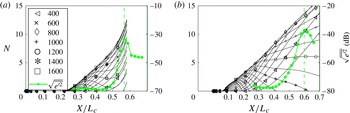
The
 $N$
-factor computations for two-dimensional TS modes (
 $k_{z}=0$
) and transition measurements on the upper and the lower side of the aerofoil,
 ${\it\alpha}=-0.60^{\circ }$
,
 $\mathit{Re}=3.142\times 10^{6}$
. Legend numbers denote frequencies
 $f$
in Hertz. (a) Upper side; (b) lower side.

In order to verify the boundary-layer stability characteristics on both sides of the wing glove, the transition measurements are complemented with results from linear stability theory (LST). For low lift coefficients the measured pressure distributions in flight correspond well (Reeh et al.
Reference Reeh, Weismüller and Tropea2014) with the results obtained with the two-dimensional aerofoil analysis program Xfoil (Drela Reference Drela and Mueller1989). The boundary conditions for the boundary-layer computations are determined with a combined experimental and numerical procedure. To increase accuracy, a fit of the computational Xfoil results to the measured pressure distribution is used in the region of high-pressure gradients close to the stagnation point region
 $X/L_{c}<0.1$
, where the limited number of pressure sensors does not provide a sufficiently resolved curve. Downstream, where the changes in the streamwise gradient are gradual, the measured pressure data are approximated by fifth-order polynomial fits. Bernoulli’s equation is used to determine the velocity distribution, which serves as the boundary condition for the boundary-layer calculations. The boundary-layer method is based on a Keller–Box discretisation (Keller Reference Keller1978; Cebeci & Cousteix Reference Cebeci and Cousteix2005; Köhler Reference Köhler2011). Local linear stability analysis (parallel flow assumption) is conducted by employing a spectral collocation method. The spanwise wavenumber
 $k_{z}$
, the angular frequency
 ${\it\omega}$
and the local Reynolds number
 $\mathit{Re}$
are prescribed as real quantities at each streamwise station. The solution of the underlying eigenvalue problem yields the modal properties of the TS wave modes. In the following the complex wavenumber
 $k_{x}=k_{x,r}+\text{i}k_{x,i}$
, the wave propagation angle
 ${\it\Psi}$
, the phase speed
 $c$
and the logarithmic amplification ratio
 $N$
(
 $N$
-factor) of the partial wave modes will be used to compare the experimental data to the predictions of LST. More details about the underlying theory and the numerical methods are given by Reeh (Reference Reeh2009, Reference Reeh2014).
Moderate deceleration or acceleration of the boundary layer has tremendous effects on boundary-layer transition. This becomes particularly clear in the two
 $N$
-factor plots in figure 7 when comparing the shape of the
 $N$
-factor curves on the upper and the lower side of the aerofoil. While the
 $N$
-factor curves on the upper side are all progressive, the frequency selective growth and attenuation of TS waves for different streamwise positions are observed for the
 $N$
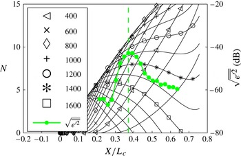
-factor curves on the lower side. The theoretical results are compared with the corresponding experimental RMS-curve from figure 6. Due to the nonlinear sensor characteristic of the array-matched surface hot films, quantitative comparison with theoretical modal amplification is not possible but the qualitative shape of the experimental curves underlines the following considerations of the influence of the streamwise pressure gradient.
Clearly, the disturbance evolution inside the boundary layer of a two-dimensional, subsonic aerofoil is highly dependent on the pressure gradient. On the upper side, after the initial acceleration of the boundary layer, the pressure recovery starts at
 $X/L_{c}\approx 0.35$
. The recovery progressively decelerates the laminar boundary layer providing grounds for strong TS wave growth in a narrow streamwise region (
 $0.45<X/L_{c}<0.65$
), which is typical when approaching the laminar separation limit (Horstmann et al.
Reference Horstmann, Quast and Redeker1989). Over a short streamwise distance nonlinear processes promote a rapid breakdown into turbulent spots (van Hest Reference van Hest1996), which is indicated by the sharp rise of fluctuation intensity shortly upstream of the maximum in the experimental RMS distributions.
In strong adverse pressure gradient flow, as it is found in the transition region on the upper side, exponential instability of TS modes dominates within localised wavepackets of small initial amplitudes until closely upstream of breakdown (van Hest Reference van Hest1996; Bech, Henningson & Henkes Reference Bech, Henningson and Henkes1998). Two-dimensional waves experience strong linear growth. In secondary instability investigations and direct numeric simulations for self-similar boundary layers and controlled disturbance input Kloker (Reference Kloker1993, Reference Kloker1995) noted that a strong adverse pressure gradient can lead to a higher efficiency of fundamental resonance (K-type, Klebanoff, Tidstrom & Sargent Reference Klebanoff, Tidstrom and Sargent1962; Kachanov Reference Kachanov1994) compared with subharmonic resonance (N-type or H-type, Kachanov & Levchenko Reference Kachanov and Levchenko1984; Herbert Reference Herbert1988), which is more efficient at low TS wave amplitudes in mildly decelerated boundary layers with a certain level of background disturbances.
For the lower side there is only a mild negative pressure gradient for the depicted flow conditions, which is slowly varying over the entire streamwise distance. TS waves thus evolve over a considerable streamwise distance. Disturbances with different spectral properties amplify at different stages, the higher-frequency
 $N$
-factor curves being the first to rise and to be damped out before reaching critical levels. This gradual growth of different spectral components promotes weakly nonlinear wave interactions (Würz et al.
Reference Würz, Sartourius, Kloker, Borodulin, Kachanov and Smorodsky2012).
In general, it is observed in figure 7 that the theoretical, two-dimensional
 $N$
-factor curves start to grow upstream of the experimentally observed amplification of the hot-film RMS signals. Owing to their limited sensitivity, the hot-films are only able to capture disturbances above a certain amplification threshold. The peak values in the RMS distributions correspond to remarkably high two-dimensional
 $N$
-factors at the position of their occurrence, which is common in flight experiments (Horstmann et al.
Reference Horstmann, Quast and Redeker1989; Reeh et al.
Reference Reeh, Weismüller and Tropea2014). The values for the upper side (
 $N\approx 11$
) and for the lower side (
 $N\approx 13$
) are not equal for the present case.
3.2.1. Determination of the disturbance propagation velocity
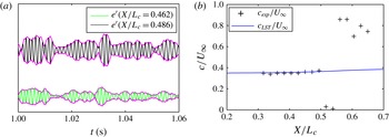
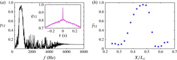
To support the statement that transition is initiated by a superposition of TS waves of different frequencies, the propagation velocity of the disturbances is determined and compared with LST. The concept of a wavepacket is understood as a localised disturbance consisting of partial waves of different frequencies, propagation angles and phase velocities. An example for a typical signal is shown in figure 8(a). The phase velocity
 $c$
of a constituent wave mode can be obtained in principle from the measurements of two closely distributed sensors. As the wavelength of some of the TS waves in the present study was less than the streamwise hot-film sensor distance of
 ${\rm\Delta}x=28~\text{mm}$
, fourth-order Butterworth filters were applied to limit the signal bandwidth to a narrow frequency band around the investigated TS mode (Kenchi et al.
Reference Kenchi, Matsubara and Toshihiko2008). The time difference between two prefiltered sensors signals was then deduced from the cross-correlation
 ${\it\varrho}_{12}$
. Figure 8(b) compares one of the most amplified two-dimensional TS modes at a frequency of
 $700~\text{Hz}$
with the results obtained from the hot-film signals using a pass band of
 $680~\text{Hz}\leqslant f\leqslant 720~\text{Hz}$
. Despite the limited temporal and spatial resolution, the theoretical and experimental phase velocities agree very well in the streamwise region
 $0.32\leqslant X/L_{c}\leqslant 0.5$
.
Procedure for determining the phase and group velocity of the TS wavepackets (lower side,
 $\bar{{\it\alpha}}=-0.92^{\circ }$
,
 $\mathit{Re}=3.215\times 10^{6}$
). (a) Hot-film signals of two consecutive sensors and their envelope on the lower side of the wing glove. (b) Streamwise distribution of the phase velocity determined from the cross-correlation of band-pass filtered signals and comparison with LST.

In a process without dissipation, the group velocity describes the velocity of the energy transport of a wavepacket in space (Boiko et al.
Reference Boiko, Grek, Dovgal and Kozlov2002). It is defined as the partial derivative of the angular frequency
 ${\it\omega}$
with respect to the modulus of the wavenumber
 $|\boldsymbol{k}|=k$
:
 $$\begin{eqnarray}c_{g}=\frac{\partial {\it\omega}}{\partial k}=c+k\frac{\partial c}{\partial k}.\end{eqnarray}$$
The sensor distance in the present case is sufficient to detect the propagation velocity of the disturbances, as dispersion needs larger distances in the aerofoil boundary layer to become significant. Yet, the typical shape of the TS wavepacket needs to be known to enable a spatiotemporal correlation of the type
 ${\it\varrho}_{12}$
. This shape is obtained by applying a discrete Fourier transform to the digitally band-pass filtered (300–2000 Hz, fourth-order Butterworth) sensor signals. Following Gaster & Grant (Reference Gaster and Grant1975), the envelope of a deterministic wavepacket can be obtained by using the real and the imaginary part of an inverse Fourier transform of the previously obtained discrete Fourier coefficients
 ${\hat{S}}$
. As the imaginary part describes a similar wavepacket shifted by
 $90^{\circ }$
in phase, the envelope is defined as the absolute value
 $$\begin{eqnarray}\tilde{s}(t)=\sqrt{\text{Re}\left(\mathop{\sum }_{n=0}^{N/2}{\hat{S}}_{n}\text{e}^{\text{i}(2{\rm\pi}f_{n}t)}\right)^{2}+\text{Im}\left(\mathop{\sum }_{n=0}^{N/2}{\hat{S}}_{n}\text{e}^{\text{i}(2{\rm\pi}f_{n}t)}\right)^{2}}.\end{eqnarray}$$
Figure 8(a) illustrates a result of the procedure for two consecutive sensor positions. Although growing in space and being displaced in time, the general shape of the envelope of the signals is retained and a good correlation between the two envelopes can be expected. In contrast to most laboratory experiments, e.g. Gaster & Grant (Reference Gaster and Grant1975), Cohen, Breuer & Haritonidis (Reference Cohen, Breuer and Haritonidis1991) or Medeiros & Gaster (Reference Medeiros and Gaster1999), the wavepackets observed in flight are not isolated but one wavepacket gradually transitions into another. To retrieve the time difference between two consecutive signals, the cross-correlation
 ${\it\varrho}_{12}$
is computed. If the envelope shapes of the investigated disturbances are similar, the correlation shows a distinct peak. The displacement of the peak from the abscissa yields the time difference
 ${\it\tau}$
necessary to compute the propagation velocity with the known sensor distance
 ${\rm\Delta}x$
. An example for an investigated flight case is included in figure 9(a). For deterministic TS waves the proposed procedure is underlined by considering the coherence between the two signals
 $$\begin{eqnarray}{\it\gamma}_{12}=\frac{|G_{12}|^{2}}{G_{11}G_{22}},\end{eqnarray}$$
where
 $G_{12}$
,
 $G_{11}$
and
 $G_{22}$
are the auto-spectral and the cross-spectral densities of two signals, i.e. the Fourier transforms of the corresponding cross and auto-correlations. As the wavepackets disperse only gradually, a strong coherence is found for the frequency band of the TS wave hump.
Procedure for determining the group velocity of the TS wavepackets (lower side,
 $\bar{{\it\alpha}}=-0.92^{\circ }$
,
 $\mathit{Re}=3.215\times 10^{6}$
). (a) Coherence
 ${\it\gamma}_{12}$
between the signals and the cross-correlation coefficient
 ${\it\varrho}_{12}$
of the two signal envelopes; (b) coherence averaged for
 $300\leqslant f\leqslant 1000~\text{Hz}$
.

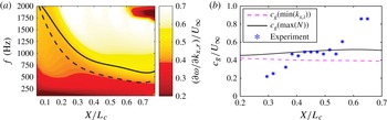
The comparison of the experimentally obtained disturbance velocity with LST is not straightforward. A ‘steepest descent’ approach would be formally correct (Schmid & Henningson Reference Schmid and Henningson2001), however, a simpler approach is chosen here for convenience. To determine the partial derivative
 $\partial {\it\omega}/\partial k$
in (3.1), the two-dimensional TS eigenvalues (
 $k_{x}=k_{x,r}+\text{i}k_{x,i}$
,
 $k_{z}=0$
) are computed for frequencies ranging from 100 to 2000 Hz in steps of 50 Hz. Hence, only the propagation in the streamwise direction is considered. The frequency distribution enables a rather smooth determination of the derivative
 $\partial {\it\omega}/\partial k_{x,r}$
for all streamwise positions, which is depicted in a contour plot in figure 10(a). Yet the desired group velocity of the TS wavepackets is given by only one value for each streamwise position. Therefore, it is assumed that the bulk of the kinetic energy is transported with the frequency producing the maximum
 $N$
-factor at each streamwise position. These positions are marked with a solid curve in the position–frequency plane in figure 10(a). Another characteristic position corresponds to the maximum disturbance growth rate
 $k_{x,i}$
, which is represented by the dashed line.
Comparison of the disturbance propagation velocity with LST results (lower side,
 ${\it\alpha}=-0.92^{\circ }$
,
 $\mathit{Re}=3.215\times 10^{6}$
). Solid line:
 $c_{g}(\max (N))$
. Dashed line:
 $c_{g}(\min (k_{x,i}))$
. (a) LST results; (b) disturbance propagation velocity.

To compare the LST results with the experimental findings, the procedure described above is used to compute the propagation velocity along the entire streamwise hot-film row on the lower side of the aerofoil. Figure 9(b) depicts the streamwise evolution of the mean coherence, which has been averaged in the frequency band 700–1000 Hz. Only in the region
 $0.38\leqslant X/L_{c}\leqslant 0.52$
is a significant coherence of
 $\bar{{\it\gamma}}_{12}>0.5$
observed. This is exactly the region where the TS hump protrudes in the spectra after overcoming the sensor noise. The coherence in figure 9(b) declines downstream when the flow randomises in the breakdown process of the boundary layer. Moreover, the comparison of the experimentally determined propagation velocities and the LST results show very good agreement in figure 10(b). The solid line corresponding to the
 $\max (N)$
criterion is closely approached by the experimental values within the coherent region. The curve corresponding to maximum modal growth describes slightly lower velocities. The characteristic propagation velocity on the lower side of the aerofoil is found at
 $c_{g}/U_{\infty }\approx 0.47$
for the non-self-similar boundary layer.
Under calm conditions, the coincidence of the frequency range of unstable modes as well as the good agreement of the propagation velocity compared with LST substantiate the assumption that transition on the wing glove is initiated by the TS type of instability.
3.2.2. Three-dimensional and nonlinear aspects of the transition process
The question of which TS-wave frequencies and propagation angles are involved in the transition process under calm conditions can be assessed by using the experimentally obtained frequency–wavenumber spectra. The hot-film data from the spanwise sensor row
 ${e^{\prime }}_{mn}=e^{\prime }(t_{m},z_{n})$
can be represented in the spectral domain by applying the discrete Fourier transform twice, first in the spanwise direction
 $z$
and then in the time domain
 $t$
. The transformation results in a two-dimensional matrix of Fourier coefficients in the discrete frequency–wavenumber domain. The resolution of the spatial wavenumber detection is limited. The maximum detectable wavenumber is determined by the Nyquist–Shannon theorem to
 $k_{z}=2{\rm\pi}/(2{\rm\Delta}z)=628.3~\text{m}^{-1}$
, where
 ${\rm\Delta}z=5~\text{mm}$
is the spanwise sensor distance. The minimum detectable wavenumber
 $k_{z}=62.8~\text{m}^{-1}$
, i.e. the largest wavelength, is determined by the length of the spanwise sensor row with 21 equidistantly distributed sensors.
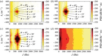
The spanwise sensor row is locally fixed and different boundary-layer states can thus only be observed by carefully changing the angle of attack. Slight changes in the angle of attack result in a deceleration or an acceleration of the lower side boundary layer and lead to the streamwise displacement of the transition process observed in figure 6. Figure 11 shows frequency–wavenumber spectra measured in flight for four different angles of attack. While the frequency axis in the contour plots scales the temporal periodicity of the signals, the spanwise wavenumber accounts for the spanwise periodicity contained in the boundary-layer disturbances. The displayed results correspond to the four different angles of attack highlighted with plus markers in figure 6(b). The superimposed lines of constant wave angles
 ${\it\Psi}$
in the first three plots were calculated using the boundary-layer method and the linear stability method described above.
Frequency–wavenumber spectra obtained with the spanwise hot-film row on the lower side: (a)
 $X/L_{c}=0.482$
,
 ${\it\alpha}=-0.16^{\circ }$
,
 $\mathit{Re}=3.032\times 10^{6}$
; (b)
 $X/L_{c}=0.482$
,
 ${\it\alpha}=-0.60^{\circ }$
,
 $\mathit{Re}=3.142\times 10^{6}$
; (c)
 $X/L_{c}=0.482$
,
 ${\it\alpha}=-0.92^{\circ }$
,
 $\mathit{Re}=3.215\times 10^{6}$
; (d)
 $X/L_{c}=0.482$
,
 ${\it\alpha}=-1.29^{\circ }$
,
 $\mathit{Re}=3.325\times 10^{6}$
.

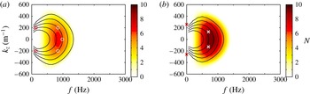
Frequency–wavenumber spectra obtained with LST. Solid lines represent contours of equal phase speed
 $c$
. From the inner to the outer curve:
 $c/U_{e}=0.31,0.33,0.35,0.37,0.39$
. Here
 $\circ$
-markers depict exemplary modal combinations for the generation of difference modes and
 $\times$
-markers depict exemplary modal combinations for streak generation: (a)
 $X/L_{c}=0.482$
,
 ${\it\alpha}=-0.60^{\circ }$
,
 $\mathit{Re}=3.142\times 10^{6}$
; (b)
 $X/L_{c}=0.482$
,
 ${\it\alpha}=-0.92^{\circ }$
,
 $\mathit{Re}=3.215\times 10^{6}$
.

For the highest angle of attack,
 ${\it\alpha}=-0.16^{\circ }$
in figure 11(a), a concentrated region of high amplitude appears for frequencies between
 $500~\text{Hz}<f<900~\text{Hz}$
and spanwise wavenumbers of
 $|k_{z}|<200~\text{m}^{-1}$
. The deviation of the maximum from the zero propagation angle is due to a slight side-slip angle of the wing glove that is consistently present, but is insignificant for the transition development. The picture of TS wavepackets with a predominant two-dimensional propagation direction is typical for a natural transition scenario in a low-disturbance environment, as can be seen in the frequency–wavenumber spectra previously obtained by Peltzer & Nitsche (Reference Peltzer and Nitsche2004) and Seitz (Reference Seitz2007) in similar flight test configurations. The corresponding wave propagation angles remain below
 $20^{\circ }$
at this early transition stage. Nevertheless, the presence of slightly oblique TS waves with different frequencies is the reason for the appearance of the localised wavepackets and the three-dimensional character of laminar–turbulent transition in the later stages. In the second case,
 ${\it\alpha}=-0.60^{\circ }$
in figure 11(b), the disturbance amplification is increased due to the increased instability of the boundary layer. Growing disturbances have spread toward higher spanwise wavenumbers, signifying an increased amplification of oblique TS waves. For
 ${\it\alpha}=-0.92^{\circ }$
in figure 11(c) the boundary layer has become even more unstable, especially toward three-dimensional modes. Besides the amplification of highly oblique TS waves at the fundamental frequencies, fluctuation energy at very low frequencies can be observed to magnify symmetrically for wavenumbers around
 $\pm 200~\text{m}^{-1}$
. Furthermore, a region of higher-harmonic waves can be seen to evolve from the background noise in the frequency band between 1300 and 1700 Hz. This indicates that the nonlinear transition stage has started. In between
 $-0.92^{\circ }\geqslant {\it\alpha}\geqslant -1.29^{\circ }$
the disturbance energy grows steeply. The spectrum fills up with fluctuation energy in-between the fundamental wave combinations and the growing low-frequency disturbances with a rich spanwise wavenumber content. For the lowest angle of attack (
 ${\it\alpha}=-1.29^{\circ }$
, figure 11
d), the low-frequency content for all spanwise wavenumbers has vastly grown. The flow is highly transitional and the disturbances are randomised. Therefore, no wave angles based on LST are included in the figure.
From these observations it can be concluded that a certain portion of three-dimensional receptivity must be involved in generating the three-dimensional modes (Kachanov Reference Kachanov2000). Furthermore, no significant nonlinear activity at the exact subharmonic wave band was detected in figure 11. At a certain amplification level of the fundamental TS waves, the power spectra fill up with fluctuation energy from the low frequency end. Furthermore, a high amplification of oblique disturbances at
 $|k_{z}|\approx 200~\text{m}^{-1}$
can be identified in the initial nonlinear transition stage. Except for a significantly weaker maximum at the first overtones of the fundamental waves, there are no other wave interactions visible in figure 11(c). The same qualitative appearance of the frequency wavenumber spectra can also be found in an article of Peltzer (Reference Peltzer2004), although the authors do not discuss this issue.
LST is employed to yield the disturbance growth rates
 $k_{x,i}$
and the phase velocity
 $c$
of all modes in the frequency–wavenumber plane (
 ${\it\omega}$
,
 $k_{z}$
) for each streamwise position. The growth rates of the three-dimensional TS modes are integrated in the streamwise direction to obtain an
 $N$
-factor distribution. In figure 12 the N-factor maximum corresponds fairly well to the experimentally observed TS wave hump in figure 11(b,c). However, disturbance growth is experimentally found even at higher spanwise wavenumbers
 $k_{z}$
. This may be explained by the fact that LST based on the parallel flow assumption underpredicts the growth of oblique wave modes, as was shown by Bertolotti (Reference Bertolotti1991).
Three-dimensional disturbances are essential for transition to turbulence in a two-dimensional boundary layer under controlled and natural forcing conditions. In the absence of visible signs of H-type or K-type wave interaction (Herbert Reference Herbert1988; Kachanov Reference Kachanov1994), the question arises: which nonlinear mechanism eventually leads to transition of the aerofoil boundary layer in a low-disturbance flight environment?
In a flat-plate experiment under different weak levels of free-stream turbulence Matsubara et al. (Reference Matsubara, Takaichi and Kenchi2010) reported two different natural transition mechanisms. For slightly higher turbulence levels they observed the expected transformation of wavepackets into
 ${\rm\Lambda}$
-shaped structures and their subsequent breakdown. For lower free-stream turbulence localised wavepackets were distorted by a short streak before rapidly breaking down. The latter scenario appears to be related to the observations of Breuer, Cohen & Haritonidis (Reference Breuer, Cohen and Haritonidis1997) in late transition stages of an isolated wavepacket in a controlled flat-plate experiment. They describe that substantial subharmonic resonance in the wavepacket is succeeded by a stage of the short but rapid streak generation. This stage was connected to the ‘oblique transition’ mechanism (Henningson, Lundbladh & Johansson Reference Henningson, Lundbladh and Johansson1993). The mechanism requires a nonlinear interaction of oblique waves to transfer energy into streamwise vortices which subsequently generate streaks through the lift-up effect (Schmid & Henningson Reference Schmid and Henningson2001). If non-modal streak growth (a linear mechanism) is sufficient, streaks become susceptible to secondary instability causing breakdown to turbulence. The first set nonlinear interaction between two oblique waves creates the modes
 $(f,k_{z})=(0,0)$
,
 $(2f_{0},0)$
,
 $(2f_{0},\pm 2k_{z,0})$
and
 $(0,\pm 2k_{z,0})$
. In the experiments of Elofsson & Alfredsson (Reference Elofsson and Alfredsson2000) and King & Breuer (Reference King and Breuer2001) the dominant energy was found for the streaks created by the stationary vortices
 $(f,k_{z})=(0,2k_{z,0})$
. However, the initial oblique waves need a certain amplitude for the nonlinear initiation of the process (Elofsson & Alfredsson Reference Elofsson and Alfredsson1998). In flight tests under low environmental disturbances such low-frequency disturbances can in principle be self-generated by non-resonant interactions of the observed broad band of TS waves and wavenumbers. One such exemplary modal combination is included in figure 12(b). Indeed, the low-frequency part of the spectrum in figure 11(c) exhibits a certain similarity to spectral representation of streaks given by Westin et al. (Reference Westin, Bakchinov, Kozlov and Alfredsson1998).
Another explanation is given by de Paula et al. (Reference de Paula, Würz, Krämer, Borodulin and Kachanov2013) who conducted a transition investigation on an aerofoil in a low-turbulence wind tunnel using a disturbance source generating fully controlled broadband frequency–wavenumber spectra. The investigation was limited to two weakly nonlinear stages of transition, i.e. no feedback influence on the fundamental TS waves, omitting explicitly the fully nonlinear state. The first stage is the generation of low-frequency waves from a simple (non-resonant) quadratic combination interaction of fundamental TS waves. Between a two-dimensional
 $(f_{1},0)$
and an oblique mode
 $(f_{2},k_{z,2})$
the first interaction set creates the modes
 $(f,k_{z})=(|f_{1}-f_{2}|,\pm k_{z,2})$
and
 $(f_{1}+f_{2},\pm k_{z,2})$
. It was shown that oblique ‘difference modes’ of the type
 $(f,k_{z})=(|f_{1}-f_{2}|,\pm k_{z,2})$
were most efficiently generated, especially when they had a phase velocity close to the one of the fundamental waves (Wu, Steward & Cowley Reference Wu, Steward and Cowley2007). Again, such a generation is plausible from the present results when comparing the amplified frequency–wavenumber content in figure 11(b,c) with figure 12(a,b), where the phase velocity
 $c$
is included by solid lines. The subsequent rapid growth of the difference modes in the non-self-similar boundary layer is described by the second stage of frequency-detuned subharmonic resonance with the fundamental waves (Würz et al.
Reference Würz, Sartourius, Kloker, Borodulin, Kachanov and Smorodsky2012). An initial broadband TS wave spectrum enables a favourable selection of the most efficient combination and a frequency cascade of this mechanism can explain the observed filling of the spectra.
Both mechanisms described above rely on a first (weakly) nonlinear stage, in which ‘seeds’ (stationary vortices or oblique low-frequency TS waves) are generated from the fundamental TS waves leading either to the subsequent creation and non-modal growth of streaks or to resonant, frequency-detuned subharmonic wave interactions. An inherent prerequisite of the first interaction mechanism is sufficient growth of the fundamental waves to generate low-frequency disturbances of significant amplitude. In figure 12 remarkably high
 $N$
-factors are reached for the parameters where the first signs of nonlinearity are observed experimentally. Hence, in a low-disturbance flight environment self-generated disturbances from the fundamental TS wave hump can assume significantly larger amplitudes than low-frequency background disturbances created directly by the receptivity of the aerofoil boundary layer. The only obvious source for the appearance of low-frequency modes is thus the self-generation by broadband interactions of the fundamental TS waves. The measurement setup in these highly challenging in-flight experiments did not have the necessary resolution to clarify completely which of the described mechanisms eventually triggers breakdown to turbulence. It can be conjectured that both mechanisms, in which combination modes of TS waves are crucial, are possible and may become important at different later stages of the transition process.
3.3. Correlation of the oncoming flow disturbances with aerofoil quantities and flight dynamics
In § 1 it was pointed out that the energy contained in atmospheric turbulence can change the flow field such that unsteady loads act on the aircraft. When investigating the effects of the oncoming flow disturbances on boundary-layer transition in-flight testing, the random nature of the turbulence complicates the investigation. The general aerofoil response is significantly different to most generic wind tunnel experiments since the boundary conditions change continuously and randomly. Correlations between flow quantities and flight dynamic quantities are therefore an indispensable prerequisite to understand the relevant processes. The need for a flawless system integration, high data acquisition rates and synchronisation of all components demonstrates the complexity of such flight experiments.
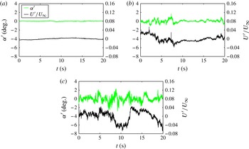
Three particular flight cases are studied which encompass most of the observed effects and serve as exemplary cases. Figure 13 shows the oncoming flow conditions for the three different categories of flight conditions. For calm conditions in figure 13(a) there are almost no fluctuations visible in the angle of attack and the velocity, which were both obtained with an X-wire probe. For the lightly turbulent conditions angle-of-attack fluctuations are smaller than
 $1^{\circ }$
. These conditions are very common in flight within the atmospheric boundary layer and can be present for the entire flight time. Clearly, variations in the chordwise velocity signal of less than 3 % and an increased fluctuation intensity on smaller scales is also apparent compared with the calm case. Reeh et al. (Reference Reeh, Weismüller and Tropea2014) show that atmospheric turbulence can be assumed isotropic for the scales relevant in aircraft flight. The third category of moderate turbulence in figure 13(c) is also frequently found in flights during daytime and it comprises angle-of-attack fluctuations smaller than
 $3^{\circ }$
. The different appearance of the angle-of-attack signal is due to the fact that it was obtained by a wind vane on the left wing of the aircraft. At the time of the measurement campaign the X-wire probes were unfortunately not available. Despite the shortcomings of the visible eigenfrequency (
 $f\approx 10~\text{Hz}$
) and the spatial distance to the wing glove this case will be particularly convenient for the depiction of boundary-layer effects in § 3.4. A fourth category, relevant to the aerodynamic performance, but less often encountered, of stronger turbulent forcing, was investigated by Weismüller (Reference Weismüller2011) in flights directly through thermals.
Different oncoming flow conditions. (a) Calm:
 ${\it\alpha}=-0.94^{\circ }$
,
 $\mathit{Re}=3.294\times 10^{6}$
. (b) Lightly turbulent:
 ${\it\alpha}=-0.95^{\circ }$
,
 $\mathit{Re}=3.520\times 10^{6}$
. (c) Moderately turbulent:
 ${\it\alpha}=-0.63^{\circ }$
,
 $\mathit{Re}=3.359\times 10^{6}$
.

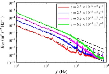
In order to enable a statistical view on the described flight cases, characteristic turbulence quantities have been derived for the three flight cases from the hotwire signals and they are presented in table 2. The turbulence intensity is based on the RMS of the band-pass filtered velocity fluctuations (second-order Butterworth transfer function, 20 Hz–2 kHz) in order to avoid any influence of the aircraft motion. This should be kept in mind when comparing the values with wind tunnel data. The energy dissipation rate is obtained by using a curve fit (power law,
 $-5/3$
) within the inertial subrange of the measured turbulence spectrum. The Kolmogorov length scale is calculated by employing the Sutherland formula for the viscosity. Details of the procedure are described by Reeh et al. (Reference Reeh, Weismüller and Tropea2014).
Comparison of characteristic turbulence quantities for different oncoming flow conditions.

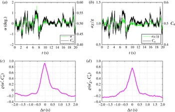
Before concentrating on the peculiarities of the transition process on the NLF aerofoil, the oncoming flow state is correlated with quantities describing the aerodynamic and flight dynamic response to the turbulent forcing. The lightly turbulent case in figure 13(b) will serve as an example since the angle-of-attack information is obtained from the boom mounted X-wire probe on the wing glove. Figure 14(a) compares the temporal evolution of the angle-of-attack fluctuations
 ${\it\alpha}^{\prime }$
with the two-dimensional normal force coefficient
 $C_{n}$
of the wing glove for the exemplary flight case. The normal force coefficient is obtained from the integral of the product between the measured pressure distribution and the normal vector along the aerofoil surface, yielding the acting pressure force vector per width which is then normalised by the dynamic head. For the non-dimensional chord-normal force component the integral can be written as the difference between the pressure coefficient
 $C_{p}=2(p-p_{\infty })/({\it\varrho}U_{\infty }^{2})$
on the lower (
 $C_{p,l}$
) and on the upper surface (
 $C_{p,u}$
) of the aerofoil:
 $$\begin{eqnarray}C_{n}=\int _{0}^{c}(C_{p,l}-C_{p,u})\,\text{d}(X/L_{c}).\end{eqnarray}$$
Cross-correlations for lightly turbulent conditions,
 $\bar{{\it\alpha}}=-0.95^{\circ }$
,
 $\bar{U}_{\infty }=41.38~\text{m}~\text{s}^{-1}$
,
 $\mathit{Tu}=0.12\,\%$
,
 ${\it\epsilon}=3.9\times 10^{-4}~\text{m}^{2}~\text{s}^{-3}$
. (a) Comparison of
 ${\it\alpha}$
and
 $C_{n}$
. (b) Comparison of
 $a_{Z}/g$
and
 $C_{n}$
. (c) Cross-correlation of
 ${\it\alpha}^{\prime }$
and
 $C_{n}^{\prime }$
. (d) Cross-correlation of
 $a_{z}^{\prime }/g$
and
 $C_{n}^{\prime }$
.

The experimental uncertainty due to the limited number of pressure taps has been evaluated with the program Xfoil (Drela Reference Drela and Mueller1989) by distributing the panel nodes according to the pressure tap positions and comparing the results with a solution obtained with a multiple number of panels. A systematic error of
 ${\rm\Delta}C_{n}=0.014$
results. Together with the integrated instrument uncertainty of the pressure sensors, a maximum measurement error of
 ${\rm\Delta}C_{n}=0.016$
is obtained.
A good correlation between the angle-of-attack fluctuations and the normal force coefficient can be expected from the time traces. In order to determine the phase lag between the signals, a cross-correlation of the two quantities is shown in figure 14(c). The cross-correlation coefficient
 ${\it\varrho}$
is normalised such that the autocorrelations of the signals are identically unity (Bendat & Piersol Reference Bendat and Piersol2010). The peak value
 ${\it\varrho}_{{\it\alpha},C_{n}}\approx 0.9$
is slightly displaced to the left from the ordinate, representing a phase lag of 29 ms. Thus, the X-wire probe 0.9 m ahead of the leading edge senses gusts earlier than the pressure distribution of the wing glove. A simple estimate using the mean free-stream velocity (
 $41.38~\text{m}~\text{s}^{-1}$
) of the present case and the quarter chord of the aerofoil (
 $c/4=0.34~\text{m}$
) leads to convection time of 30 ms, which is in good agreement with the present measurements.
In order to demonstrate the accuracy of the sensor synchronisation, figure 14(b,d) show a cross-correlation between the normal force coefficient and the dimensionless chord-normal acceleration, which was obtained by the AHRS inside the wing glove described in § 2.2. Again a high correlation coefficient results and this time the phase lag is essentially zero, as it is smaller than the sampling period of the AHRS which obtains the accelerometer data at a rate of 100 Hz.
The correlations clearly demonstrate that the loads on the aerofoil result from the oncoming flow disturbances and are not pilot induced. In addition, the time scales of the transient disturbances are too small to allow intuitive pilot reactions. The gusts in the oncoming flow field create rapid changes of the aerofoil pressure distribution which determine the dominating force component normal to the chord. It will be shown in the following section how the boundary layer responds to these variations of the boundary conditions.
3.4. Investigation of time-dependent boundary-layer transition
In order to obtain a general view of the temporal transition development, the signal of each streamwise hot-film sensor is divided into overlapping segments (50 %) of 0.1 s, resulting in 1600 samples for statistical averaging and yielding a statistical value for every 0.05 s. By this procedure time-varying RMS values of the hot-film signals for each time window of the 20 s measurement sequence are obtained. It generates the graphics in figure 15, which are easy to interpret. The three-dimensional contour plots illustrate the spatiotemporal evolution of the disturbance amplification inside the boundary layer. The nonlinearity of the hot-film response may influence the growth quantitatively but not qualitatively. The transition process is always marked by a steep increase of the hot-film RMS values. Both sides of the aerofoil are depicted for the moderately turbulent oncoming flow conditions in figure 13(c). The time-dependent RMS values reveal remarkable differences between the upper and the lower side of the aerofoil.
Spatiotemporal transition development on both sides of the wing glove under moderately turbulent conditions, mean flow quantities:
 ${\it\alpha}=-0.63^{\circ }$
,
 $\mathit{Re}=3.359\times 10^{6}$
. (a) Upper side; (b) lower side.

On the upper side, variations of the amplification onset are limited in their streamwise extent to
 ${\rm\Delta}X/L_{c}\leqslant 0.1$
. Although peak-to-peak fluctuations of the angle of attack of almost
 $3^{\circ }$
are observed in figure 13(c), transition on the upper side of the particular aerofoil is clearly fixed in this narrow streamwise region. The reason is the evolution of the pressure gradient, which for all instantaneous flow states only becomes strongly adverse in the region
 $0.4\leqslant X/L_{c}\leqslant 0.6$
. There it leads to a strong deceleration of the boundary layer, which causes high disturbance amplification. Only for mean angles of attack
 ${\it\alpha}>3^{\circ }$
does this situation change, as the deceleration of the boundary layer moves significantly upstream. However, these cases are beyond the scope of the present investigation. Furthermore, it can be construed from this observation that no obvious sign of bypass transition was found for the investigated mean angles. Bypass transition due to direct entrainment of free-stream turbulence would not depend as strongly on the adverse pressure gradient (Boiko et al.
Reference Boiko, Grek, Dovgal and Kozlov2002). Thus, disturbance amplification is clearly confined to the region
 $0.4\leqslant X/L_{c}\leqslant 0.6$
, where TS modes experience the highest growth rates according to LST, as it was observed in figure 7(a).
Figure 15(b) for the lower side appears remarkably different. At several time instances very rapid changes in the streamwise position of the disturbance amplification occur. Upstream and downstream excursions of the transition front of
 ${\rm\Delta}X/L_{c}>0.2$
result on very short time scales
 ${\rm\Delta}t<0.5~\text{s}$
. It should be recalled from the quasi-steady considerations in § 3.2 that for negative angles of attack the lower side boundary layer decelerates, promoting the growth of TS waves, but for increasing angles of attack the TS waves are more and more damped.
3.4.1. The role of the instantaneous pressure gradient
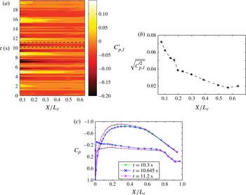
To check the validity of the above considerations, the role of the pressure gradient on the lower side is investigated in detail. Figure 16(a) shows the temporal fluctuations of the pressure coefficient
 $C_{p}^{\prime }$
obtained with the miniature pressure sensors on the lower side of the wing glove in the streamwise region between
 $0.07\leqslant X/L_{c}\leqslant 0.64$
. Fluctuations of
 $\pm 0.15$
are observed for short time periods and changes in the sign of the pressure coefficient become apparent. The variations are intensified in the leading-edge region which is underlined by the RMS values of the pressure fluctuations included in figure 16(b). Whereas positive deflections generally lead to a stabilisation of the boundary layer, negative deflections have a destabilising effect on the lower side of the wing section. It can be observed that the upstream fluctuations of boundary-layer disturbance growth in figure 15(b) correspond to negative deflections of the pressure coefficient
 $C_{p,l}$
in figure 16(a) at approximately the same time. Note that these results qualitatively correlate with the quasi-steady expectations in figure 6.
Fluctuations of the pressure coefficient on the lower side: (a) temporal fluctuations; (b) RMS of
 $C_{p}^{\prime }$
on the lower side; (c) instantaneous pressure distributions due to a downward directed gust.

Thus, to some extent the fluctuating transition position in figure 15 can be explained by the quasi-steady considerations in § 3.2. Yet, the characteristic time scales of some of the observed transition excursions are of the order of
 $0.2~\text{s}\leqslant {\rm\Delta}t\leqslant 1~\text{s}$
in the present experiments, which will be further verified in § 3.4.1. Within such periods the aerofoil travels only a distance corresponding to 6–30 chord lengths. For such dimensionless distances the time derivatives assume an important role in the conservation equations (Bisplinghoff et al.
Reference Bisplinghoff, Holt and Halfman1996). The relevance of unsteady inviscid aerofoil effects as well as unsteady boundary-layer effects can be assessed more clearly when considering these time periods as half-cycles of an oscillation and by determining the characteristic frequency of a corresponding harmonic excitation. Table 3 provides an estimation of these relations, including the reduced frequency
 ${\it\kappa}$
(McCroskey Reference McCroskey1982) and the boundary-layer frequency parameter
 ${\it\kappa}_{{\it\delta}}$
(Lighthill Reference Lighthill1954; Hill & Stenning Reference Hill and Stenning1960; Patel Reference Patel1975). Both dimensionless numbers express ratios between the fluid convection time scale and the time scale of a harmonic excitation caused by the oncoming flow or the outer flow of the boundary layer, respectively. According to Leishman, Rycroft & Shyy (Reference Leishman, Rycroft and Shyy2006) unsteady inviscid effects become significant for
 ${\it\kappa}>0.05$
and they consider
 ${\it\kappa}>0.2$
highly unsteady. Note that unsteady distortions of the boundary-layer profiles compared with the quasi-steady case increase with the boundary-layer length (
 ${\it\kappa}_{{\it\delta}}\propto x$
), which is significant for the investigated aerofoil (Patel Reference Patel1975; Reeh Reference Reeh2014).
Estimation of dimensionless time and frequency scales to characterise the unsteadiness of the aerofoil flow (
 $U_{\infty }$
,
 $L_{c}=1.35$
,
 $x\approx X$
).

For an unsteady outer flow, the boundary condition for the boundary-layer development, i.e. the unsteady edge velocity, cannot solely be determined from the surface pressure since Bernoulli’s equation contains the time derivative of the velocity potential. It was already inferred from figure 15 that the variation of the pressure gradient plays an outstanding role for the boundary-layer development and affects transition. In order to demonstrate typical amplitudes observed in these transient events, characteristic instantaneous pressure distributions for one such event at
 $10.3~\text{s}\leqslant t\leqslant 11.2~\text{s}$
are depicted in figure 16(c). A strong deviation of
 ${\rm\Delta}C_{p}$
is observed at
 $t=10.645~\text{s}$
, especially in the leading edge part. The deflection corresponds to the aerofoil response to a downward directed gust. On the lower side of the aerofoil
 ${\rm\Delta}C_{p,l}\geqslant 0.2$
and the pressure gradient at this particular time instant is completely adverse, promoting a significant deceleration of the boundary layer. The distributions for
 $t=10.3~\text{s}$
and
 $11.2~\text{s}$
almost coincide. In the following it will be shown that the duration of the bulk of the deflection occurs in less than
 $0.4~\text{s}$
.
3.4.2. Investigation of the streamwise excursions of the transition front
The striking rapidness of some of the upstream transition fluctuations with durations of less than 0.3 s in figure 15(a) calls for a more profound investigation in order to determine their nature. Considering the increased level of small-scale turbulence in the oncoming flow (cf. figure 13 c and table 2), the spectral composition of these transition excursions is of particular interest. Studer et al. (Reference Studer, Arnal, Houdeville, Seraudie and Govindarajan2006) showed in a low-disturbance wind tunnel that the unsteady boundary-layer development on an aerofoil can significantly affect the transition mechanism. Their results show the rapid appearance of turbulent bursts which are preceded by nonlinear instabilities. The mechanism was first described by Obremski & Fejer (Reference Obremski and Fejer1967) in an experimental study of an oscillating flat-plate boundary layer. Tani (Reference Tani1969) and Loehrke, Morkovin & Fejer (Reference Loehrke, Morkovin and Fejer1975) explain the occurrence of such transition by the rapid quasi-steady growth of linear instability waves travelling through unsteadily distorted, highly unstable boundary-layer profiles.
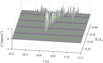
Figure 17 shows the temporal variations of the AC part of the hot-film raw signals for such a transition excursion (
 $10.2~\text{s}<t<11.2~\text{s}$
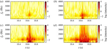
, from the first to the eighth sensor of the streamwise hot-film row). This time span is marked with dashed lines in figure 15(b). The voltage signals of the considered time sequence have been normalised with the maximum value observed in the considered time sequence. The highly nonlinear transition stage appears as sudden bursts of high amplitudes, which marks the course of the transition excursion. Starting the consideration of the plot at
 $t\approx 10.4~\text{s}$
,
 $X/L_{c}=0.42$
and proceeding in time, transition moves upstream until reaching a minimum streamwise position at
 $t\approx 10.64~\text{s}$
. Continuing along the timeline from this upstream position, the transition front moves downstream again and reaches the last depicted sensor in less than 0.1 s. Before and after the excursion of the transition front, localised waveforms are visible at the downstream positions indicating that the transition front spends more time in this region. Yet, only strong low-frequency, nonlinear modulations can be observed in the depicted time interval. According to figure 7(b), amplified TS waves are expected at significantly higher frequencies (700–1500 Hz). Completed breakdown and homogenised turbulence can only be observed downstream of the sensor position
 $X/L_{c}=0.353$
within the time interval of the transition excursion.
Surface plot of the spatiotemporal disturbance evolution of a transition excursion. Lines depict the normalised hot-film signals. Positions for the wavelet analysis are marked with thick lines.

The time period over which the transition excursion appears corresponds to the
 $C_{p,l}$
fluctuations shown in figure 16, which reach a minimum at approximately the same time when the transition front reaches its most upstream position. A minimum in
 $C_{p,l}$
leads to a deceleration of the boundary layer in the present flight case. It can be inferred from these considerations that boundary-layer transition is mainly driven by the pressure gradient under these disturbed flow conditions. It is important to note that the coherence between the movement of the transition front and the excursions in the pressure gradient excludes the possibility of a pure bypass transition from a convective disturbance generated by free-stream turbulence.
3.4.3. Wavelet analysis of the temporal transition fluctuations
The high nonlinearity at streamwise positions far upstream of the mean transition region calls for deeper insight into the spectral properties of the process to determine whether it starts linearly or whether it is intrinsically nonlinearly. The appearance of the transition front excursion is highly localised in space and time. Conventional Fourier analysis, which is conceptually delocalised in time, may not shed sufficient light into all of the details involved in the time–frequency domain. Therefore, wavelet analysis is employed to investigate the transient process. The use of this method is inspired by the works of Hudgins, Friehe & Mayer (Reference Hudgins, Friehe and Mayer1993), Studer et al. (Reference Studer, Arnal, Houdeville, Seraudie and Govindarajan2006) and Bernardini et al. (Reference Bernardini, Benton, Chen and Bons2013), who also applied wavelet analysis in transient boundary-layer flows. Since the important basics of wavelets are presented in each of these studies and further information can be found in the review of Farge (Reference Farge1992), only a brief summary of the most important aspects of the continuous wavelet transform applied in the present case is given. The transform can be interpreted as an inner product between an analysing function, i.e. the wavelet, and the signal to be analysed. It is defined by the integral
 $$\begin{eqnarray}{\hat{W}}(a,{\it\tau})=\frac{1}{\sqrt{a}}\int _{-\infty }^{\infty }e^{\prime }(t){\it\psi}^{\ast }\left(\frac{t-{\it\tau}}{a}\right)\,\text{d}t.\end{eqnarray}$$
The function
 ${\it\psi}^{\ast }$
denotes the complex conjugate of the wavelet which is intrinsically localised in time. It can be compressed or stretched by the scale parameter
 $a$
and shifted in time by the parameter
 ${\it\tau}$
to approximate locally the function
 $e^{\prime }(t)$
to be analysed. In order to be admissible for the transform, the analysing function
 ${\it\psi}$
needs to fulfill certain mathematical requirements (Farge Reference Farge1992). The strength of wavelet analysis is that a great variety of analysing functions exists and a suitable one can be chosen depending on the particular physical process. Here, a Morlet wavelet is used for its good representation of sine-like signal parts as they are expected due to determinism involved in boundary-layer transition:
 $$\begin{eqnarray}{\it\psi}(t)=\sqrt{{\rm\pi}b}\exp \!\left(\text{i}2{\rm\pi}f_{c}t\right)\exp \!\left(-\frac{t^{2}}{b}\right).\end{eqnarray}$$
The wavelet function constitutes a plane wave modulated by a Gaussian envelope. The scales used in wavelet analysis cannot directly be connected to frequencies in the Fourier sense. The maximisation of a given wavelet with a sine wave yields the centre frequency
 $f_{c}$
. In (3.5) the scale parameter
 $a$
is connected to the centre frequency
 $f_{c}$
of the Morlet wavelet by the relation
 $f_{p}=f_{c}/a$
, where
 $f_{p}$
is the so-called pseudo-frequency. In the present application of the Morlet wavelet the pseudo-frequency is a good approximation of the real frequency. The scales
 $a$
are prescribed as
 $1/\log (a)$
in order to obtain a favorable distribution of pseudo-frequencies between 1 Hz and 8 kHz important for the present investigation. The resulting wavelet coefficients
 ${\hat{W}}$
from (3.5) yield the energy spectrum
 ${\hat{W}}\hat{W^{\ast }}=|{\hat{W}}^{2}|$
, which represents the energy content of the signal in the time-scale domain or the time-pseudo-frequency in the present case.
In figure 18 the result of the wavelet analysis is demonstrated for the four different streamwise positions marked in figure 17, corresponding to the second, fourth, sixth and the eighth streamwise sensor. Maybe the most important insight into the transition mechanism can be inferred from the contour plot in figure 18(a) at the first streamwise station. Only a small portion of the time–frequency domain contains energy. At
 $t\approx 10.6~\text{s}$
and within the frequency band of 500–1800 Hz disturbances are amplified. The concentration in a particular frequency band suggests that transition is indeed initiated by a linear amplification process of TS waves before the start of the nonlinear evolution. For the second station at
 $X/L_{c}=0.287$
short-time nonlinear processes can already be observed by the broader frequency distribution approximately at the same time when the transition front reaches the most upstream position. Yet, the energy transfer occurs on a very short time scale. At earlier and later time instants, amplification of the linear fundamental frequencies is observed. Further downstream, the nonlinear stage at
 $X/L_{c}=0.331$
and
 $X/L_{c}=0.375$
covers longer time periods. The last streamwise station in figure 18(d) includes the homogenisation of turbulence at
 $t\approx 10.65~\text{s}$
and another nonlinear amplification can be observed at
 $t\approx 10.95~\text{s}$
. The nonlinear stage in figure 18(b–d) is preceded and followed by amplification in the TS wave band.
Contours in logarithmic scale of the normalised wavelet coefficient depicting the disturbance energy in the time–frequency domain at four streamwise positions: (a)
 $X/L_{c}=0.242$
; (b)
 $X/L_{c}=0.287$
; (c)
 $X/L_{c}=0.331$
; (d)
 $X/L_{c}=0.375$
.

Comparison of transition measurements with quasi-steady N-factor computations, which are based on the instantaneous pressure distribution at
 $t=10.65~\text{s}$
in figure 16(c). Legend numbers denote frequencies
 $f$
in Hz.

From these results it can be concluded that the transient appearance of the ‘transition flashes’ is associated with the transient development of the laminar boundary layer which is driven by rapid changes of the flow field along the boundary-layer edge. These changes are mainly caused by vertical gusts and the resulting aerofoil motion in flight through moderate atmospheric turbulence, as demonstrated in the study of Reeh et al. (Reference Reeh, Weismüller and Tropea2014). A pure bypass transition attributed to an entrainment of free-stream turbulence can be excluded from the present results. Nevertheless, a combined effect of unsteady boundary-layer development and higher small-scale free-stream turbulence forcing on transition cannot be excluded. In their generic wind-tunnel experiments, Studer et al. (Reference Studer, Arnal, Houdeville, Seraudie and Govindarajan2006) investigated two frequencies of periodic pressure gradient changes in an aerofoil boundary layer. Their ‘low-frequency’ case exhibits strong similarities to the present results. In their ‘high-frequency’ case, the unsteady boundary-layer effects were strong enough to cause transition by the convection of a turbulent front after formation of an initial turbulent spot. This type of transition, first discovered by Obremski & Fejer (Reference Obremski and Fejer1967), is not observed in the present flight cases.
Quasi-steady
 $N$
-factor calculations are conducted for this event to demonstrate differences in the obtained transition
 $N$
-factors with calm flight conditions. The computations are based on the instantaneous pressure distribution. Note that the most amplified frequencies correspond to the observations of the wavelet spectra in figure 18. For the depicted time instant
 $t=10.65~\text{s}$
the hot-film RMS curve is based on 1600 samples corresponding to an averaging interval of
 ${\rm\Delta}t=0.1~\text{s}$
. The
 $N$
-factor corresponding to the peak RMS distribution is found to be
 $N\approx 10.5$
. In comparison with the findings under calm conditions in figure 7(b) a reduction of
 ${\rm\Delta}N\approx 3$
is observed. Despite the observed reduction, the comparably high
 $N$
-factor of
 $N=10.5$
still substantiates a dominant role of TS waves in the transition process.
Two systematic errors are introduced by employing quasi-steady boundary-layer computations based on the instantaneous pressure distribution. First, the contribution of the time derivative in the Bernoulli equation to the velocity distribution necessary for the boundary-layer computation cannot be accounted for (Reeh Reference Reeh2014). Second, the role of unsteady distortions of the boundary-layer profiles is neglected as the time history of the boundary-layer development is completely omitted by the quasi-steady procedure (Hill & Stenning Reference Hill and Stenning1960; Patel Reference Patel1975). The impact of both effects on the present results needs to be assessed in future numerical investigations using unsteady computation methods. The quasi-steady application of linear stability methods for transition prediction is still justified since the frequencies of the observed TS waves are about two orders of magnitudes higher than the frequencies associated with the unsteady aerofoil response, a reasoning which is also pointed out by Obremski & Morkovin (Reference Obremski and Morkovin1969).
3.4.4. Some remarks on the effects of small-scale turbulence
The presence of TS waves in all investigated cases, which is also observed by Zanin (Reference Zanin1985) in flights at even higher turbulence intensities, is explained by the relatively weak vortex receptivity processes found on a typical laminar wing section. Considering the elevated turbulence intensity levels in flight through moderately turbulent conditions (
 $\mathit{Tu}\leqslant 0.4\,\%$
), the question whether this forcing is able to create stronger TS waves in the receptivity process is of importance. When drawing comparisons with wind-tunnel experiments, it should be recalled that the turbulence encountered in the in-flight experiments is intrinsically different to wind-tunnel turbulence of nominally similar turbulence intensity levels. For the considered aerofoil boundary layer, the waveband relevant for TS waves amplification is
 $300~\text{Hz}\leqslant f\leqslant 2~\text{kHz}$
. Figure 20 shows flight-measured kinetic energy spectra for low turbulence intensities. The dashed lines represent the one-dimensional form Kolmogorov’s power law for the inertial subrange used in conjunction with Taylor’s hypothesis
 $$\begin{eqnarray}E_{XX}(f)=\frac{U_{\infty }}{2{\rm\pi}}C_{T,X}\,{\it\epsilon}\,f^{-5/3},\end{eqnarray}$$
where
 $C_{T,X}=0.66$
is a universal turbulence constant for the one-dimensional energy spectrum (Sheih, Tennekes & Lumley Reference Sheih, Tennekes and Lumley1971). The energy containing eddies of atmospheric turbulence, i.e. those motions involved in the turbulence generation, are generally produced on length scales of the order of a hundred metres. Therefore, the bulk of the kinetic energy of the turbulence is contained at length scales which are irrelevant for boundary-layer receptivity. In the cascade process of atmospheric turbulence, kinetic energy decays over at least two decades before reaching the TS wave frequencies. Most of the directional information is lost and the statistics of the motion becomes universal. This is a major difference to most wind-tunnel investigations, where a certain degree of anisotropy is inevitable (Westin et al.
Reference Westin, Boiko, Klingmann, Kozlov and Alfredsson1994) and may influence the type of boundary-layer disturbances (Kendall Reference Kendall1998). Furthermore, the wind-tunnel turbulence spectrum may be entirely different (Zanin Reference Zanin1985; Weismüller Reference Weismüller2011). In the TS waveband ordinary wind tunnels may create stronger fluctuations. It is therefore deemed plausible that the TS wave dominated transition scenario can persist at higher nominal
 $\mathit{Tu}$
values in flight than under common wind-tunnel conditions. Note further that most comparable wind-tunnel studies are conducted for lower flow speeds, where the instability of the boundary layer is also found at lower frequencies. Nevertheless, the comparison in figure 20 shows that the energy density available for the generation of boundary-layer disturbances differs over all relevant frequencies for different turbulence conditions.
Comparison of one-dimensional turbulence spectra measured by means of hotwire anemometry in gliding flight at low turbulence levels.

Along the boundary layer, the inherently three-dimensional and localised disturbances imposed by free-stream turbulence can continuously feed energy for the generation of TS wavepackets (Kachanov Reference Kachanov2000). However, the convection velocity of free-stream turbulence components is higher than the phase velocity of the TS modes and at given TS frequencies a wavelength reduction is necessary to transfer energy. An energy transfer can be promoted by interactions of external vorticity with localised or distributed surface roughness creating disturbances matching TS waves in their vital aspects, i.e. amplitude, wavenumbers and frequency (Crouch Reference Crouch1992a ,Reference Crouch b ; Dietz Reference Dietz1999; Saric et al. Reference Saric, Reed and Kerschen2002). On a polished wing surface, however, such receptivity sites are largely avoided and Bertolotti (Reference Bertolotti1997) shows that free-stream turbulence components corresponding to the TS wave band do not penetrate efficiently into lower part of the boundary layer, where TS waves exhibit an amplitude maximum. Furthermore, any TS waves created by a leading edge receptivity mechanism are dampened significantly before reaching the point of neutral stability. The previous results and considerations infer a relatively weak influence of atmospheric turbulence on TS wave amplitudes.
Bertolotti (Reference Bertolotti1999) considers a direct coupling of lower-frequency turbulence components to streaky disturbance structures very efficient. The evolution of these Klebanoff modes is directly connected to the transient growth mechanism (Matsubara & Alfredsson Reference Matsubara and Alfredsson2001; Schmid & Henningson Reference Schmid and Henningson2001) and various experiments (Kendall Reference Kendall1985; Boiko et al. Reference Boiko, Westin, Klingmann, Kozlov and Alfredsson1994; Westin et al. Reference Westin, Boiko, Klingmann, Kozlov and Alfredsson1994; Matsubara & Alfredsson Reference Matsubara and Alfredsson2001; Fransson et al. Reference Fransson, Matsubara and Alfredsson2005; Kenchi et al. Reference Kenchi, Matsubara and Toshihiko2008) have shown that this coupling mechanism has a crucial importance for higher turbulence levels than those encountered in this investigation. The present experimental set-up did not allow a detailed investigation into the possible generation of low-frequency Klebanoff modes. Nevertheless, the typical features of a TS wave initiated transition scenario have been demonstrated under all investigated flight conditions. As explained in §§ 3.4.1 and 3.4.3, no indication of bypass transition was found. On both sides of the aerofoil, streamwise excursions of the transition front were triggered by fluctuations of the pressure gradient. Disturbance amplification is clearly confined to the region, where TS modes experience the highest growth rates according to LST. Hence the boundary-layer response to the natural disturbances supports the dominant role of TS waves in the transition process. The question whether streaky disturbance structures are also present and modify the transition process in gliding flight through atmospheric turbulence needs to be assessed in future studies.
4. Conclusions
In the present work a comprehensive measuring system for the investigation of the effects of atmospheric turbulence on a NLF wing section has been presented. Based on the experience of previous in-flight studies, the system has been enhanced considerably in order to gain deeper insights into the flight physics, especially the boundary-layer transition process. Under calm flight conditions, the influence of the angle of attack on transition was examined on the upper and the lower side of the NLF aerofoil. A characteristic quasi-steady behaviour of each side was deduced for the boundary conditions prevailing in flight through atmospheric turbulence. Furthermore, the consideration of spanwise frequency–wavenumber spectra enabled an interpretation of the linear transition development under real, calm flight conditions. The relevance of the spanwise distribution of boundary-layer disturbances for the weakly nonlinear transition stage on a NLF aerofoil was considered in detail. Similarities of the observed transition process with the wind-tunnel experiments of Matsubara et al. (Reference Matsubara, Takaichi and Kenchi2010) and de Paula et al. (Reference de Paula, Würz, Krämer, Borodulin and Kachanov2013) were described and the importance of self-generated disturbances was highlighted.
In flights through atmospheric turbulence it was shown that the forcing has sufficient energy to influence significantly the loads and the flight dynamics of the aircraft. Cross-correlations between the oncoming flow and the aerofoil response showed that the effects were created by velocity fluctuations in the free stream. Pilot-induced variations could be excluded due to the very rapid changes in the flow quantities with durations of less than 0.2 s. Whereas laminar–turbulent transition on the upper side of the wing section fluctuated by
 ${\rm\Delta}X/L_{c}\approx 0.1$
, the transition process on the lower side was found to be highly dependent on the time-varying boundary conditions induced by the turbulent oncoming flow. It created unsteady boundary-layer characteristics that influenced the disturbance growth and lead to upstream fluctuations of transition of more than
 ${\rm\Delta}X/L_{c}=0.2$
. Wavelet analysis was used to obtain insights into the mechanism of the rapid upstream shifts of transition on the lower side of the aerofoil. From the results it could be inferred that the observed short-time upstream excursions of the transition front result mainly from temporal variations of the boundary-layer profiles. As in the lower-frequency case of the investigations of Studer et al. (Reference Studer, Arnal, Houdeville, Seraudie and Govindarajan2006), these short-time variations can promote very strong instability growth but the transition process was shown to start with linear, modal amplification of TS waves at first. Considerations on the importance of small-scale turbulence components were presented.
Acknowledgements
The authors express their thanks to their students M.Sc. T. Hartmann, M.Sc. T. W. Martins, B.Sc. M. Bonnert, B.Sc. F. Tenzer, O. Ikonnikova and T. Hofmann. Without their ongoing unweary help the comprehensive and challenging flight experiments would not have been possible. The authors are particularly indebted to Dipl.-Ing. A. Güttler and Dipl.-Ing. D. Wolfram for their continuous support. This work was supported by the Deutsche Forschungsgemeinschaft (DFG) under the grant TR 194/48-2.