Nomenclature
-
 $A({x_r})$
-
Membership function for input variable
${x_r}$
-
$a_{z}$
-
vertical accelerations, g
- b
-
wing span, m
-
$C_{x}$
, C
z
, C
m
-
longitudinal aerodynamic force and moment coefficients
-
$C_{y}$
, C
l
, C
n
-
lateral-directional aerodynamic force and moment coefficients
-
$\bar c$
-
mean aerodynamic chord, m
- h
-
altitude, m
-
$I_{xx}, I_{yy}, I_{zz}$
-
moments of inertia about x-, y-, and z-axes, respectively, kg·m2
-
$I_{xy}, I_{xz}, I_{yz}$
-
products of inertia, kg·m2
-
$k_{\textit{1}}$
,
$k_{\textit{2}}$
-
longitudinal and lateral-directional reduced frequencies, respectively
- L, M, N
-
moments acting about the (x, y, z)-body axes of aircraft, respectively, N · m
- M
-
Mach number
- m
-
aircraft mass, kg
- p, q, r
-
body-axis roll rate, pitch rate, and yaw rate, deg./s.
- PMic
-
pitching moment due to inertia coupling
- RMic
-
rolling moment due to inertia coupling
- YMic
-
yawing moment due to inertia coupling
-
$\bar q$
-
dynamic pressure, kpa
- R 2
-
square of multiple correlation coefficients
- S
-
wing reference area, m2
-
$T_{x}$
-
thrust term along the x-body axis of the aircraft, N
-
$T_{m}$
-
thrust term in the pitching equation of motion, N
- t
-
time, sec
- T, W
-
thrust and aircraft weight in flight, N, respectively
- X, Y, Z
-
forces acting on the aircraft body-fixed axes along x-, y-, and z-axes, N, respectively
-
$\alpha, \dot \alpha $
-
angle-of-attack, deg. and time rate of change of angle-of-attack, deg./sec., respectively
-
$ \beta, \dot{\beta} $
-
sideslip angle, deg. and time rate of change of sideslip angle, deg./sec., respectively
-
$\delta_{a}, \delta_{e}, \delta{r} $
-
control deflection angles of aileron, elevator and rudder, respectively, deg.
-
$\phi,\theta,\psi $
-
Euler angles in roll, pitch, and yaw, respectively, deg.


1.0 Introduction
Clear-air turbulence with hard-to-detect characteristics has been an important factor to endanger flight safety. The transport aircraft in flight is subjected severe clear-air turbulence resulting with the abrupt change in attitude and gravitational acceleration (i.e. the normal load factor). These varying characteristics not only pose threats to flight safety, but also may cause structural damages and reduce fatigue life [Reference Chang, Ye, Lan and Guan1]. Since the sudden plunging motion frequently causes injuries to passengers and crew members, it is important to provide training program of control strategy for loss-of-control prevention for the pilots in the airlines. These effects of varying response characteristics are quite difficult to be simulated by wind-tunnel tests or conventional flight simulators.
According to the statistics of the International Civil Aviation Organisation (ICAO), the causes of accidents due to weather factors were about 30%, but it accounted for more than $65.8 million USD/year lost to airlines of turbulence-related injuries to cabin crew ([2]. An intersecting zone of tropical and frigid air currents causes large-scale air movements due to the different densities of hot and cold air. It is easy to form clear-air turbulence at high atmospheric altitude in the case of uneven convection [Reference Hamilton and Proctor3]. Many clear-air turbulence related occurrences of transport aircraft happen in North-east Asia, especially on en-route turbulence over the ocean near Japan during cruise flight.
The hazardous levels of turbulence involving the plunging motion of the transport aircraft were determined to sense the severity of turbulence in references of Sheu and Lan 2011 [Reference Sheu and Lan4] and Chang 2013 [Reference Chang5]. The turbulence hazard index in terms of the damping value of plunging mode and the integrated turbulence-induced downwash was discussed in references of Sheu and Lan 2011 [Reference Sheu and Lan4]. To prevent flight injuries, the turbulence hazard intensity in terms of the damping value of plunging mode would be more reliable. However, to have a proper correlation between RMS normal load and flying quality intensity, more cases are needed.
The evaluations of stability characteristics for transport aircraft in severe clear-air turbulence based on aerodynamic derivatives extracted from fuzzy-logic aerodynamic models were demonstrated in reference to flying qualities for a twin-jet transport in severe atmospheric turbulence [Reference Chang, Ye, Lan and Guan1]. Although the fuzzy-logic aerodynamic models have robustness and nonlinear interpolation capability in predicting the degradation in stability and control characteristics, it can’t provide neither the flight control strategy in avoidance of injuries nor the training program in loss-of-control prevention for the airlines. To examine the possible mitigation concepts of accident prevention, the application of nonlinear dynamical inversion and a new study of flight control strategy are undertaken. This paper employs flight data mining and the fuzzy-logic modeling (an artificial intelligence technique), to establish nonlinear flight controllability models based on post flight data. This transport aircraft encountered severe clear-air turbulence twice during the descending phase [Reference Chang5]. The flight control strategy can be obtained from nonlinear and unsteady flight controllability models through flight simulations of dynamic inversion process. Then, the hazardous mitigation can be determined based on the influences of longitudinal in lateral-directional attitudes. The necessary and appropriate applications to improve the flight controls of rudder, aileron and elevator during severe clear-air turbulence will be demonstrated.
2.0 Flight data mining technology
The input data for fuzzy-logic modeling is extracted from post-flight data. There are many flight parameters recorded by FDR (flight data recorder), but some of them are not related to the current study, such as light signs, landing gear retracting and so on. The steps are to collect and organise a large amount of data and obtain the required information from them for specific analysis and applications; this process is so called flight data mining [Reference Han, Kamber and Pei6]. The flight data mining process is divided into three parts: the developments of a non-linear unsteady aerodynamic database, platform development of root cause summary in loss of control (including aerodynamic-model setup) and platform development of flight control strategy in loss of control prevention (including flight dynamic-model setup).
2.1 Development of nonlinear and unsteady aerodynamic database
This section describes the development process of data manipulation, compatibility check, input information of aircraft main geometry and moment of inertia data, equations of motion, and unsteady thrust model. The flowchart for development of a non-linear and unsteady aerodynamic database is shown in Fig. 1.
Flowchart for development of a non-linear unsteady aerodynamic database.

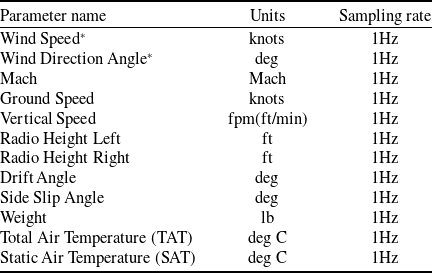
Raw data of flight status (I)

*Required dataset.
Raw data of flight status (II)

*Required dataset.
2.1.1 Data manipulation
Before developing a non-linear and unsteady aerodynamic database, one must ensure that the selected parameters and corresponding data are the required data for study. The parameters and corresponding data required for current study include the following items:
-
1) To select the required flight status, flight control surface, and engine raw data extract from a specific flight number of actual flight QAR or FDR data. The required parameter names, reference units, and reference sampling rates are shown in Tables of 1–4.
-
2) The thrust performance of the entire aircraft is non-public data and must be obtained from the Flight Planning and Performance Manual (Boeing Series) or Flight Crew Operation Manual (Airbus Series).
Supplementary note:
-
(1) The parameters marked with an asterisk in Tables 1–4 are necessary parameters. If lacking, it will make the development of the database difficult.
-
(2) The parameters marked with # in the table above are necessary parameters that can be replaced with each other. At least one of them must exist. If all of them are absent, the development of the data warehouse will be difficult.
-
(3) If the data of the same name is divided into CAPT and F/O, CAPT is the main factor; if it is divided into CMD and ACTUAL, the ACTUAL will prevail.
The frequency of each parameter sensor is different from 1Hz to 8Hz due to the properties and characteristics of the parameters. For example, attitude angles such as roll, pitch and heading angles are 4Hz in Table 1; aileron and elevator angles are 2Hz in Table 3; the vertical acceleration sampling rate is 8Hz in Table 1. To preserve the properties and characteristics of each parameter, it is necessary to avoid high frequency data loss, so the frequency of all original data sampling is uniformly arranged to 8Hz.
Raw data of flight control surface

Raw data of engine

The data frequency increase and data make up of this research is developed based on the method of monotone cubic spline interpolation [Reference Wolberg and Alfy7]. This curve fitting method is commonly used in aircraft flight test analysis to provide a smooth curve. Data upscaling and data completion of blanks are important steps for aerodynamic database to have high accuracy and reliability in applications to operational efficiency enhancement of transport aircraft.
2.1.2 Compatibility check
Typically, the longitudinal, lateral and vertical accelerations (
 $a_{x}$
,
 $a_{y}$
,
 $a_{z}$
) along the (x, y, z)-body axes of aircraft, angle-of-attack
 $\alpha$
, Euler angles (
 $\phi$
,
 $ \theta$
, and
 $\psi$
), aileron deflection (
 $ \delta_{\textrm{a}}$
), elevator (
 $ \delta_{\textrm{e}}$
), rudder (
 $ \delta_{\textrm{r}}$
), stabiliser (
 $ \delta_{\textrm{s}}$
) and so on are available and recorded in the QAR of all transport aircraft. Since the recorded flight data may contain errors (or called biases), compatibility checks are performed to remove them by satisfying the following kinematic equations [Reference Lan, Wu and Yu8, Reference Dadios9]:
 \begin{equation}\dot \phi = p + q\sin \phi \tan \theta + r\cos \phi \tan \theta \end{equation}
 \begin{equation}\dot \theta = q\cos \phi - r\sin \phi \end{equation}
 \begin{equation}\dot \psi = \left( {q\sin \phi + r\cos \phi } \right)\!\sec \theta \end{equation}
 \begin{equation}\dot V = \left({a_x} - g\sin \theta \right)\!\cos \alpha \cos \beta + \left( {{a_y} + g\sin \phi \cos \theta } \right)\!\sin \beta + \left( {{a_z} + g\cos \phi \cos \theta } \right)\!\sin \alpha \sin \beta \end{equation}
 \begin{equation}\dot \alpha = \frac{{\left[ {\left( {{a_z} + g\cos \theta \cos \phi } \right)\!\cos \alpha - \left( {{a_x} - g\sin \theta } \right)\!\sin \alpha } \right]}}{{(V\cos \beta )}} + q - \tan \beta \!\left( {p\cos \alpha + r\sin \alpha } \right)\end{equation}
 \begin{align}\dot \beta = & \frac{{\cos \beta \!\left( {{a_y} + g\cos \theta \sin \phi } \right)}}{V} + p\sin \alpha - r\cos \alpha\nonumber\\[5pt]& - \sin \beta \!\left[ {({a_z} + g\cos \theta \cos \phi } \right)\!\sin \alpha - ({a_x} - g\sin \theta )\!\cos \alpha ]/V\end{align}
where g is the gravitational acceleration and V is the flight speed. Let the errors be denoted by
 ${b_{{a_x}}},{b_{{a_y}}},{b_{{a_z}}},{b_p},{b_q},{b_r},{b_V},{b_\alpha },{b_\beta },{b_\theta },{b_\varphi },{b_\psi }$
, respectively for
 $a_{x}$
,
 $a_{y}$
,
 $a_{z}$
, etc. These errors are estimated by minimising the squared sum of the differences between the two sides of Equations 2.1–2.6.
These equations in vector form can be written as:
 \begin{equation}\dot{{\mathop z\limits^{\rightharpoonup}}} = {\mathop f\limits^{\rightharpoonup}} \!\left( {\mathop x\limits^{\rightharpoonup}} \right) = {\mathop f\limits^{\rightharpoonup}} \big( {{{\mathop x\limits^{\rightharpoonup}} }_m} - \Delta {\mathop x\limits^{\rightharpoonup}} \big)\end{equation}
where
 \begin{equation}{\mathop z\limits^{\rightharpoonup}} = {\left( {V,\bar \alpha ,\bar \beta ,\theta ,\phi ,\psi } \right)^T}\end{equation}
 \begin{equation}{{\mathop x\limits^{\rightharpoonup}} _m} = {\left( {{{\bar a}_x},{{\bar a}_y},{{\bar a}_z},\bar p,\bar q,\bar r,V,\bar \alpha ,\bar \beta ,\theta ,\phi ,\psi } \right)^T}\end{equation}
 \begin{equation}\Delta {\mathop x\limits^{\rightharpoonup}} = {\left( {{b_{{a_x}}},{b_{{a_y}}},{b_{{a_z}}},{b_p},{b_q},{b_r},{b_V},{b_\alpha },{b_\beta },{b_\theta },{b_\phi },{b_\psi }} \right)^T}\end{equation}
where overbar “-” stands for the mean value and the subscript “m” indicates the measured or recorded values. The cost function is defined as:
 \begin{equation}J = \frac{1}{2}{\Big( {\dot{\mathop z\limits^{\rightharpoonup}} - {\mathop f\limits^{\rightharpoonup}} } \Big)^T}Q\Big( {\dot{\mathop z\limits^{\rightharpoonup}} - {\mathop f\limits^{\rightharpoonup}} } \Big)\end{equation}
where Q is a weighting diagonal matrix with elements being 1.0 and
 $\dot {\mathop z\limits^{\rightharpoonup}} $
is calculated with a central difference scheme with
 ${{\mathop z\limits^{\rightharpoonup}} _m}$
, which is the measured value of
 ${\mathop z\limits^{\rightharpoonup}} $
. The steepest descent optimisation method is adopted to minimise the cost function. Some variables and errors in Equations (2.9) and (2.10) are unavailable in the QAR/FDR can be estimated through compatibility checks.
The above-mentioned unavailable variables and errors in the QAR, need initial values as a basis for correction, where the angular rates, such as p, q and r are obtained from derivatives of
 $\varphi $
,
 $\theta $
and
 $\Psi $
with time by using the method of monotonic cubic interpolation. This interpolation method is used to connect the flight data into a continuous curve to obtain the slope of the curve. The value of
 $\beta$
cannot be obtained from the derivative. The initial value of
 $\beta$
is assumed to be 0 at the time of estimation, and it is calculated when the Equation 2.6 is satisfied.
2.1.3 Aircraft main geometry and moment of inertia data
The force and moment coefficients in equations of motion for the transport aircraft under the study require to input the information of aircraft main geometry and moment of inertia data. The transport aircraft under the study is a twin-jet (underwing engines) transport aircraft. The data of main geometry and moments of inertia for this transport aircraft are presented in Table 5. Those are public data of aircraft manufacturers and can be obtained via the Internet or flight operation manual.
Main geometry and moment of inertia data for the twin-jet (underwing engines) transport aircraft

2.1.4 Equations of motion
The actual physical phenomenon of an aircraft flying in the atmosphere is the movement along the flight trajectory over time. Since all flight variables recorded are based on the body axes, it is more convenient to estimate the force and moment coefficients for aircraft on the same axes system. The following equations of motion are derived based on the textbook of Roskam 2018 [Reference Roskam10]:
-
(1) force coefficients acting on the body axes of the aircraft
(2.12)
\begin{equation}m{a_x} = {C_x}\bar qS + {T_x}\end{equation}
(2.13)
\begin{equation}m{a_y} = {C_y}\bar qS + {T_y}\end{equation}
(2.14)
\begin{equation}m{a_z} = {C_z}\bar qS + {T_z}\end{equation}
-
(2) moment coefficients about the body axes of the aircraft
(2.15)
\begin{equation}{C_l}\bar qSb = {I_{xx}}\;\dot p - {I_{xz}}\dot r + qr\!\left( {{I_{zz}} - {I_{yy}}} \right) - {I_{xz}}pq\end{equation}
(2.16)
\begin{equation}{C_m}\bar qS\bar c = {I_{yy}}\dot q + rp\!\left( {{I_{xx}} - {I_{zz}}} \right) + {I_{xz}}\!\left( {{p^2} - {r^2}} \right) - {T_m}\end{equation}
(2.17)
\begin{equation}{C_n}\bar qSb = - {I_{xz}}\;\dot p + {I_{zz}}\dot r + pq\!\left( {{I_{yy}} - {I_{xx}}} \right) + {I_{xz}}qr\end{equation}


where m is the aircraft mass;
 $\bar q$
is the dynamic pressure; S is the wing reference area; b is the wing span;
 $\bar c\;$
is the mean aerodynamic chord;
 $C_{x}$
,
 $C_{z}$
and
 $C_{m}$
are the longitudinal aerodynamic force and moment coefficients;
 $C_{y}$
,
 $C_{l}$
and
 $C_{n}$
are the lateral-directional aerodynamic force and moment coefficients; and
 $I_{xx}$
,
 $I_{yy}$
, and
 $I_{zz}$
are the moments of inertia about x-, y-, and z-axes, respectively. The products of inertia,
 $I_{xy}$
,
 $I_{xz}$
and
 $I_{yz}$
, are assumed zero in the present case; but are included in the equations because non-zero values may be available in other applications. The terms,
 $T_{x}$
,
 $T_{y}$
,
 $T_{z}$
and
 $T_{m}$
, represent the thrust contributions to the force in the direction of x-, y-, z-axes, and to the pitching moment, respectively.
 $T_{m}$
is a thrust-moment term about y-axis due to underwing engines, giving a nose-up moment, so the sign convention is negative in Equation (2.16).
In Equations (2.15)–(2.17), pq, qr and pr are the product terms of two dependent variables or
 ${p^2},{r^2}$
are the square terms of a variable; those are non-linear terms in mathematics. The squared terms of a variable, along with nonlinearity in the aerodynamics, are the dominant non-linear terms in the differential equations of motion. Therefore, Equations (2.15) to (2.17) belong to the nonlinear differential equation system. Non-linear differential equations are very difficult to solve mathematically, and the physical phenomena of motion are more complicated [Reference Sugar-Gabor11]. In the physical sense, the product term of the two dependent variables is related to each other, which is the coupling effect of nonlinear motion. To compute the aerodynamic coefficients — given the motion variables which can be obtained from the QAR/FDR. The development process of non-linear unsteady aerodynamic database has four steps. The data manipulation is the first step; it includes the demand data selection, data frequency upscaling and data make up. Thrust data prediction is the second step; a numerical model ties up the recorded engine performance parameters in Table 4 and flight operation manual to develop the thrust model by using the fuzzy-logic algorithm. Compatibility check is the third step; it performs to remove biases of recorded flight data and to estimate
 $\beta$
, p, q and r by satisfying the kinematic equations. Input required information is the fourth step, it includes the data of main geometry and moments of inertia for the study transport aircraft.
The terms on the left side of Equations (2.15)–(2.17) are rolling, pitching and yawing moments, respectively. The moments due to inertia coupling on the right side in Equations (2.15)–(2.17) will be produced due to the abrupt change in the flight attitude before and during the severe clear-air turbulence encounters.
The third term on the right side of Equation (2.15) is the rolling moment (RMic) due to inertia coupling as follows:
 \begin{equation}\textrm{R}{\textrm{M}_{\textrm{ic}}} = \textrm{qr}\!\left( {{\textrm{I}_{\textrm{zz}}}-{\textrm{I}_{\textrm{yy}}}} \right)\end{equation}
The product of qr in Equation (2.18) represents pitch rate coupling with yaw rate, so as, the pitching moment (PMic) and yawing moment (YMic) due to inertia coupling are also presented as follows:
 \begin{equation}\textrm{P}{\textrm{M}_{\textrm{ic}}} = \textrm{rp}\!\left( {{\textrm{I}_{\textrm{zz}}}-{\textrm{I}_{\textrm{xx}}}} \right)\end{equation}
 \begin{equation}\textrm{YMic} = \textrm{pq} (\textrm{Iyy}-\textrm{Ixx}) \end{equation}
2.1.5 Unsteady thrust model
 ${T_x}$
,
 ${T_y}$
,
 ${T_z}$
,
 ${T_m}$
are the axial thrusts along body x-, y-, z-coordinate and pitching moment about y-axis, respectively, in Equations (2.12)–(2.14), and (2.16). It can be known from the various thrusts that the force and moment acting on the aircraft will be affected by the engines. Both thrust and aerodynamic forces are generated together, and the two effects cannot be accurately separated only from the flight record data during analysis. To accurately estimate the aerodynamic coefficient, it is necessary to obtain an accurate thrust value to separate the thrust effects, and then the accurate aerodynamic coefficients can be obtained [Reference Lan, Wu and Yu8].
Since the values of thrust for aircraft in flight cannot be directly measured in the current state of the art, they are neither recorded in the QAR nor FDR. The actual thrust in operation is obtained by using the recorded variables from Table 4 and engine’s thrust change curves are adopted from flight manual. The engine’s thrust change curves tabularised in numerical datasets to associate with the recorded variables in Table 4 are the input data files for numerical thrust model establishment. Therefore, the present thrust model is an unsteady state.
In the present study, the fuel flow rate (
 ${\dot m_f}$
) at various altitude (h), weight (W), Mach number (M), calibrated airspeed (CAS), engine pressure ratio (EPR) in cruise flight adopted from the flight manual are utilised. The flight operation manual has the required lists and graphs of engine efficiency changes with altitude and speed, these data can be used to complete the engine’s thrust change curves.
For the Pratt & Whitney turbofan engines, thrust (T) is defined by EPR, so that the thrust model is set up as:
 \begin{equation}T = f\!\left( {h,W,M,CAS,EPR, {{\dot m}_f}} \right)\end{equation}
For General Electrical (GE) or CFM International (CFM) turbofan engines, the rpm of the low-pressure compressor (
 $N_{\textit{1}}$
) is used to set the level of thrust, so that the thrust model is set up as:
 \begin{equation}T = f\!\left( {h,W,M,CAS,{N_1},{{\dot m}_f}} \right)\end{equation}
A twin-jet with GE turbofan engines in the present paper will be illustrated.
Theoretically, clear-air turbulence (i.e. random change in u, w (or
 $\alpha$
) and v (or
 $\beta$
) affect the engine performance through its effects on static and dynamic distortions at the engine face. However, its effects are not known and cannot be estimated, and therefore ignored in the present application.
Once the thrust model is generated as a function of h, W, M, CAS, EPR and with the flight conditions of climbing, cruise and descent, one can obtain the accurate aerodynamic coefficients after breaking away the thrust effects.
2.2 Platform development of root cause summary in loss of control
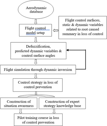
This section describes the development of root caused analysis in loss of control, as shown in Fig. 2. The flowchart of Fig. 2 is based on the data of the non-linear unsteady aerodynamic database. The fuzzy logic modeling technique is used to set up aerodynamic models. The non-linear unsteady aerodynamic model can provide the stability and controllability derivatives to be used for the event analyses. The derivative indices can help to pinpoint the major cause more efficiently while proceeding event or accident investigation, to judge about how difficult it was for the pilot or the autopilot system to control the aircraft in severe clear-air turbulence.
Flowchart for platform development of root cause summary in loss of control.

2.2.1 Non-Linear unsteady aerodynamic models
When studying the non-linear unsteady aerodynamic characteristics of motion, it can be found that the non-linear unsteady aerodynamics with hysteresis [Reference Chang5, Reference Lan, Wu and Yu8] are affected by many parameters of motion state. The aerodynamic models developed by the fuzzy-logic modeling method is suitable for aerodynamic research of coupling motion and can be used to enhance the operational efficiency of transport aircraft.
Modeling means to establish the numerical relationship among certain variables of interest. In the fuzzy-logic model, more complete necessary influencing flight variables can be included to capture all possible effects on aircraft response to structure deformations. The longitudinal main aerodynamics is assumed to depend on the following ten flight variables [Reference Lan, Wu and Yu8]:
 \begin{equation}{C_x},{C_z},{C_m} = f\!\left( {\alpha ,\dot \alpha ,q,{k_1},\beta ,{\delta _e},M,p,{\delta _s},\bar q} \right)\end{equation}
The coefficients on the left-hand side of Equation (2.23) represent the coefficients of axial force (
 $C_{x}$
), vertical force (
 $C_{z}$
), and pitching moment (
 $C_{m}$
), respectively. The variables on the righthand side of Equation (2.23) denote the angle-of-attack (
 $\alpha$
), time rate of angle-of-attack (d
 $\alpha$
/dt, or
 $\dot \alpha $
), pitch rate (q), longitudinal reduced frequency (
 $k_{\textit{1}}$
), sideslip angle (
 $\beta$
), control deflection angle of elevator (
 $ \delta_{e} $
), Mach number (M), roll rate (p), stabiliser angle (
 $\delta_{s}$
) and dynamic pressure (
 $\bar q$
). These variables are called the influencing variables. The roll rate is included here because it is known that an aircraft encountering hazardous weather tend to develop rolling which may affect longitudinal stability. The variable of dynamic pressure is for estimation of the significance in structural deformation effects. The qualitative evaluations of flight dynamic characteristics are based on the first derivatives of longitudinal stability and control effectiveness, and the second derivatives is utilised to examine the static aeroelastic effects.
For the lateral-directional aerodynamics [Reference Lan, Wu and Yu8],
 \begin{equation}{C_y},{C_l},{C_n} = f\!\left( {\alpha ,,\beta ,\phi ,p,r,{k_2},{\delta _a},{\delta _r},M,\dot \alpha ,\dot \beta } \right)\end{equation}
The coefficients on the left-hand side of Equation (2.24) represent the coefficients of side force (
 $C_{y}$
), rolling moment (
 $C_{l}$
) and yawing moment (
 $C_{n}$
), respectively. The variables on the right side of Equation (2.24) denote the angle-of-attack (
 $\alpha$
), sideslip angle (
 $\beta$
), roll angle (
 $\phi$
), roll rate (p), yaw rate (r), lateral-directional reduced frequency (
 $k_{\textit{2}}$
), control deflection angle of aileron (
 $\delta_{a}$
), control deflection angle of rudder (
 $\delta_{r}$
), Mach number (M), the time rate of angle-of-attack (
 $\dot \alpha $
) and the time rate of sideslip angle (
 $\dot \beta $
).
2.2.2 Aerodynamic and damping derivatives
The most representative of numerical differentiation theory is the difference method. This paper uses the central difference method to take the derivative. The central difference method to obtain the derivative is to take the differential point as the centre point, and respectively select a value close to 0 from the left and right of the differential point to compare, and obtain the derivative of the certain point.
Assuming a function f(x), if one wants to find the derivative at the point x, take x as the centre point and select the value of the distance between the left and right sides close to 0, namely f(x+) and f(x–), and then find the Taylor expansion and the principle of the central difference method are as follows:
Taylor expansion to find f(x +
 $\Delta x$
):
 \begin{equation}f(x + \Delta x) = f(x) + f^\prime (x)\Delta x + \frac{{{f^{(2)}}(x)}}{2}\Delta {x^2} + \ldots ..\end{equation}
Taylor expansion to find f(x –
 $\Delta x$
):
 \begin{equation}f\!\left( {x + \Delta x} \right) = f(x) + f^\prime (x)\Delta x + \frac{{{f^{(2)}}(x)}}{2}\Delta {x^2} + \cdots \end{equation}
Taylor expansion to find f(x –
 $\Delta x$
):
 \begin{equation}f\!\left( {x - \Delta x} \right) = f(x) + f^\prime (x)\left( { - \Delta x} \right) + \frac{{{f^{(2)}}(x)}}{2}{({-} \Delta x)^2} + \cdots \end{equation}
Then,
 \begin{equation}f\!\left( {x - \Delta x} \right) = f(x) - f^\prime (x)\Delta x + \frac{{{f^{(2)}}(x)}}{2}\Delta {x^2} + \cdots \end{equation}
Subtracting (2.26) from (2.28), one gets
 \begin{equation*}f\!\left( {x + \Delta x} \right) - f\!\left( {x - \Delta x} \right) = 2f^\prime (x)\Delta x\end{equation*}
 \begin{equation}\textrm{Therefore},\ f^\prime (x) = \frac{{f\!\left( {x + \Delta x} \right) - f\!\left( {x - \Delta x} \right)}}{{2\Delta x}}\end{equation}
Although the above-mentioned numerical differentiation method is used to obtain the derivative of a certain point of the function curve, in fact, it can also be applied to the derivative analysis of flight data. However, some flight data are scattered and have discontinuous points, the least square method is applied to connect the points into a continuous smooth curve. The predicted results of fuzzy-logic models can generate smooth coefficient curves with the required independent variables to provide reasonable local aerodynamic derivatives [Reference Chang5].
The tangent slope of a point on the curve is the derivative value of this point. Add and subtract a small same value to the abscissa value of this point, respectively, corresponding to the slope of the line connecting two points on the curve, which is calculated by the finite difference method. Fuzzy-logic modeling is extremely important in the aerodynamic performance analysis of actual flight data. Here are two examples of applying the fuzzy-logic modeling model to take derivatives:
The longitudinal stability derivative (
 $C_{m\alpha}$
) comes from the model of
 $C_{m}$
. The aerodynamic derivative of the unsteady aerodynamic model can be calculated using the central interpolation method. The formula of the central difference method is as follows:
 \begin{equation}{C_m}_{\alpha} = [{C_m}({\alpha} + \Delta{\alpha}, \hbox{- - -} ) - {C_m}({\alpha} - \Delta {\alpha}, \hbox{- - -} )]/2\Delta {\alpha}\end{equation}
 $\Delta\alpha = 0.1$
degrees mean that
 $\alpha$
changes up and down by 0.1 degrees, while all other variables remain unchanged.
The damping derivative
 $(\textrm{C}_{\textrm{lp}})$
is proposed from the model Cl. The formula of the central interpolation method is as follows:
 \begin{equation}{\textrm{C}_{\textrm{lp}}} = [{\textrm{C}_{\textrm{l}}}( \hbox{- - -} ,\textrm{p}\Delta \, + \,\textrm{p}, \hbox{- - -} ) - {\textrm{C}_{\textrm{l}}}( \hbox{- - -} ,\textrm{p} - \Delta \textrm{p}, \hbox{- - -} )]/2\Delta \textrm{p}\end{equation}
Where Δp is in unit of deg/sec.
The calculations of all other aerodynamic derivatives are derived from the same method in this paper.
The effectiveness criteria for derivative values of stability, damping and controllability are shown in Table 6. The root cause analysis for aircraft accident due to the pilots in loss of control are based on assessment of stability, damping and controllability in flight dynamics. The magnitude values of these three derivatives are the judgement criteria for effectiveness.
The effectiveness criteria for derivative values of stability, damping, and controllability

Remarks: The effectiveness is judged based on the positive or negative of derivative value.
2.3 Platform development of flight control strategy in loss of control prevention
The purpose of this section is to obtain the flight control strategy through appropriate flight simulation by using the flight control main models of the elevator, aileron and rudder with the nonlinear dynamic inverse function. The platform development of flight control strategy in loss of control prevention is also based on the data of the non-linear unsteady aerodynamic database, as shown in Fig. 3. The fuzzy logic modeling technique is used to set up flight control models.
Flowchart for platform development of flight control strategy in loss of control prevention.

The non-linear unsteady flight control model can provide the predicted deflected angles of flight control surfaces, static and dynamic variables related to root cause summary in loss of control. Dynamic inversion in this section plays the role of flight simulation in loss of control prevention as a tool to support the decision making of flight control strategy. The constructions of situation awareness and expert strategy knowledge bases require more study cases; these parts will be the future tasks in our research team.
2.3.1 Non-linear unsteady flight controllability model
A preprocessor is needed to rearrange the flight variables in the datasets of FDR and interpolate the variables if it is necessary by a monotone cubic spline [Reference Wolberg and Alfy7]. The FDR data can provide the necessary data to develop models for aviation accident analysis [Reference Chang, Ye, Lan and Guan1, Reference Chang5] and pilot training [Reference Lan, Wu and Yu8]. If flight test data are used, no further interpolation is necessary in most cases [Reference Brandon, Lan, Li and Wang12].
The following numerical models based on the FDR data in flight operation with clear-air turbulence encountering may be generated:
 \begin{equation}{\delta _a} = {f_1}\!\left( {\alpha ,\theta ,\phi ,\dot \phi ,\dot \psi ,\dot \theta ,{V_{cas}},{a_z},{a_y},{V_{crw}},{V_{tlw}},RMic} \right)\end{equation}
 \begin{equation}{\delta _r} = {f_1}\!\left( {\alpha ,\theta ,\phi ,\dot \phi ,\dot \psi ,\dot \theta ,{V_{cas}},{a_z},{a_y},{V_{crw}},{V_{tlw}},YMic} \right)\end{equation}
 \begin{equation}{\delta _e} = {f_1}\!\left( {\alpha ,\theta ,\phi ,\dot \phi ,\dot \psi ,\dot \theta ,{V_{cas}},{a_z},{a_y},{V_{crw}},{V_{tlw}},PMic} \right)\end{equation}
where the parameter on left side of Equations (2.32) – (2.34) represents the aileron angle (
 $\delta_{a}$
), rudder angle (
 $\delta_{r}$
) and elevator angles (
 ${\delta _e}$
). The flight variables on the right side represent angle-of-attack (
 $\alpha$
), pitch angle (
 $\theta $
), roll angle (
 $\phi $
), time rate of roll angle (
 $\dot \varphi $
), time rate of heading angle (
 $\dot \psi $
), time rate of pitch angle (
 $\dot \theta $
), calibrated airspeed (
 ${V_{cas}}$
), vertical accelerations (
 $a_{z}$
), lateral acceleration (
 $a_{y}$
), crosswind speed (V
crw
), tailwind speed (V
tlw
), rolling moment due to inertial coupling (RMic), yawing moment due to inertial coupling (YMic) and pitching moment due to inertial coupling (PMic). Since the accident event doesn’t have abrupt change in longitudinal acceleration, so the above influencing flight variables of flight control model development exclude a
x
.
To develop flight controllability models, one or more dynamic variables (on the right sides of the above expressions) are chosen as the enabling variables to achieve the desired dynamics. Traditionally, the flight controls are usually developed based on the rates on the rotating axes (i.e. “p”, “q” and “r”). In the present case, the time rates of roll angle, yaw angle and pitch angle (
 $\dot \varphi $
,
 $\dot \theta $
and
 $\dot \psi $
) are used, because it will provide damping directly to the Euler angle-motion. This is particularly important when
 $\phi$
,
 $\dot \varphi $
and
 $\dot \psi $
have large amplitudes in roll oscillation. In the sudden plunging motion,
 $\dot \theta $
is the enabling variable because it is the response directly related to elevator. However, associated with the specified change in
 $\alpha$
, the lateral acceleration (
 $a_{y}$
) and vertical accelerations (
 $a_{z}$
) should be changed as well. Therefore, the following sub-models are needed associated with Equation (2.34):
 \begin{equation}\alpha = {f_{11}}\!\left( {\theta ,\phi ,\dot \phi ,\dot \psi ,\dot \theta ,{V_{cas}},{a_y},{V_{crw}},{V_{tlw}},PMic} \right)\end{equation}
 \begin{equation}{a_y} = {f_{12}}\!\left( {\alpha ,\theta ,\phi ,\dot \phi ,\dot \psi ,\dot \theta ,{V_{cas}},{a_z},{V_{crw}},{V_{tlw}},PMic} \right)\end{equation}
 \begin{equation}{a_z} = {f_{13}}\!\left( {\alpha ,\theta ,\phi ,\dot \phi ,\dot \psi ,\dot \theta ,{V_{cas}},{a_y},{V_{crw}},{V_{tlw}},PMic} \right)\end{equation}
The above influencing flight variables in sub-model development do not have a x either due to no abrupt change in longitudinal acceleration for study.
2.3.2 Flight simulation in loss of control prevention
The nonlinear dynamic inversion relates to the control instruction algorithm formed by the adjustment for the important variables of the nonlinear dynamical control, which is used to describe the function relationship between the values of controlled variables and input variables. The technique of nonlinear dynamic inversion has been very successful in the tracking control of nonlinear dynamical systems, such as a continuation design framework for nonlinear flight control problems [Reference Richardson and Lowenberg13], quadrotor with complementary fuzzy logic compensator [Reference Rodić and Stojković14] and automatic longitudinal flight controller [Reference Alam and Celikovsky15].
In the present paper, the objective of the nonlinear dynamic inversion is to provide good damping in Euler angle-motion, and then to improve flight control deflections. The three variables are described as follows [Reference Lan and Chang16]:
 \begin{equation}\mathop \sum \limits_{x + \dot x} \!\left[ {b + \left( {x - b} \right){f_c}} \right] \to {\delta _x}\end{equation}
where the summation means to combine the changes in the enabling variable (x), such as roll angle (
 $\phi$
), and its associated time rate of change; b is the specified minimum value of “x” and f
c
is the fraction to keep “x” above the minimum. The arrow sign implies dynamic inversion to determine the required control. The reason for doing this is to make the variation smooth so that the control is also smooth to avoid early control saturation.
The purpose of this study is to obtain the flight control strategy through appropriate flight simulation by using the numerical main models of the elevator, aileron and rudder with the nonlinear dynamic inverse function. The adjustment of the input b values to obtain control strategy in flight operations is important in the flight simulation. The input b value can be roll angle, time rate of roll angle, pitch angle, or time rate of pitch angle. The prediction procedures of flight simulation are described as follows:
-
1) The first, using aileron control as an example, objective: to reduce the roll angle (
$\phi$
) and improve the roll damping by selecting b = 2.0 and f
c
= 0.1. In other words, the amount of
$\phi$
above 2.0 deg is multiplied by 0.1. For
$\dot \varphi $
, the amount above 2.0 deg/sec is also multiplied by 0.1. Since rolling is always accompanied by yawing, so that
$\dot \psi $
is treated in the same way as
$\dot \varphi $
. -
2) The aileron control needed to achieve the objective in 1) is calculated through the flight control model representing Equation (2.32).
-
3) If there are sub-models, then to estimate the values of these sub-models due to the change in 1).
-
4) Check whether the control exceeds the positive and negative limits. If true, revise the factors “b” and “
$f_{c}$
”. -
5) The prediction procedures of rudder and elevator in flight simulation are the same as the procedures of 1) – 4).


The application of nonlinear dynamical inversion can mitigate the abrupt change in attitude and provide flight control strategy in loss of control prevention.
2.4 Fuzzy-logic modeling algorithm
Since the aerodynamic and flight control models are established by using flight data, modeling technique is important and need to be carefully considered. Factors that affect the modeling procedures include the mathematical tool to set up system model and the method to identify parameters of model structure. Modeling procedures start from separating the input data into many groups, and nonlinear relations are set up between each input-output data space. To obtain continuous variations of predicted results, the present method is based on the internal functions, instead of fuzzy sets [Reference Karasan, Ilbahar, Cebi and Kahraman17], to generate the output of the model.
The fuzzy-logic algorithm can take advantage of correlating multiple parameters without assuming explicit functional relations among them [Reference Dang, Vermeiren, Dequidt and Dambrine18, Reference Shi, Wang, Yang, Jian and Bi19]. The algorithm employs many internal functions to represent the contributions of fuzzy cells (to be defined later) to the over-all prediction. The internal functions are assumed to be linear functions of input parameters as follows [Reference Lan and Chang16]:
 \begin{equation}{P^i} = {y_i}\!\left( {{x_1},{x_2}, \cdots ,{x_r}, \cdots {x_k}} \right) = P_0^i + P_1^i{x_1} + \cdots + P_r^i{x_r} + \cdots P_k^i{x_k}\end{equation}
Where
 $p_r^i$
, r = 0, 1, 2,…, k, are the coefficients of internal functions
 ${y_i}$
, and k is number of input variables. In Equations (2.39),
 ${y_i}$
is the estimated aerodynamic coefficient of force or moment, and
 ${x_r}$
are the variables of the input data. The numbers of the internal functions (i.e. cell numbers) are quantified by the membership functions.
With the internal function chosen in a linear form, the fuzzy-logic model resembles the multiple linear regression method. In Equation (2.39),
 ${y_i}$
is the estimated aerodynamic coefficient of force or moment, and
 ${x_r}$
are the variables of the input data. The parameters of the input data in internal functions are extracted from aerodynamic database, so the internal functions can be linear functions of input parameters. The final predicted results of fuzzy-logic aerodynamic models are numerical data. Therefore, the governing Equations (2.12) – (2.17) can be solved through the process of fuzzy-logic modeling.
The fuzzy-logic model is a form of fuzzy cell structure composed of linear equations to make it unique. In other words, there are different numbers of cells corresponding to each input parameter. The values of each fuzzy variable, such as the angle-of-attack, are divided into several ranges, each of which represents a membership function [Reference Lan and Chang16] withas its membership grade, like a weighting factor. A fuzzy cell is formed by taking one membership function from each variable. The total number of cells is the number of possible combinations by taking one membership function from each input variable. For every cell, it has a fuzzy rule to guide the input and output relations. The rule of the i-th cell [Reference Alam and Celikovsky15] is stated as:
if x
1 is
 $A_1^i({x_i})$
, and x
2 is
 $A_2^i({x_i})$
, and … , and x
k
is
 $A_k^i({x_k})$
, then the cell output can be stated as Equation. (2.39).
where i = 1, 2, …, n the index of the cells, n is the total number of cells of the model; P
i
(x
1, x
2, …, x
r
, . . ., x
k
) is the internal function with parameters
 $p_0^i,p_1^i, \ldots ,p_r^i, \ldots ,p_k^i$
to be determined, and
 $A_k^i({x_k})$
denotes the membership function for x
k
. Each function covers a certain range of input variables.
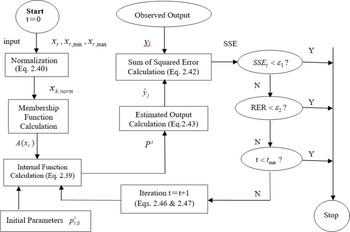
Flowchart of refining process for fuzzy-logic modeling is presented in Fig. 4. This flowchart includes input, normalisation, membership function calculation, internal function calculation and so on. Modeling refinement is used to refine the model by having all data records employed in the optimisation. The model is optimised to have high correlation coefficient.
Flowchart of refining process for fuzzy-logic modeling.

For a given system with input variables
 ${x_1},\;{x_2},\; \ldots {x_r},\;{x_k}$
of one data point, the recorded values of each input variables are normalised by using
 \begin{equation}{x_{r,norm}} = \frac{{{x_r} - {x_{r,min}}}}{{{x_{r,max}} - {x_{r,min}}}}\;, = 1,2, \cdots ,k\end{equation}
Hereafter
 ${x_{r,norm}}\;$
is denoted by x
r
for simplicity in description. The membership grading ranges are transformed into the domain [0, 1]; “0” meaning no effect from the corresponding internal function, and “1” meaning full effect. Generally, overlapped triangles are frequently the shapes used to represent the grades. A fuzzy cell is formed by taking one membership function from each variable. The output of the fuzzy-logic model is the weighted average of all cell outputs.
In each fuzzy cell, the contribution to the outcome (i.e. the cell output) is based on the internal function, Equation (2.39). The final prediction of the outcome is the weighted average of all cell outputs after the process of reasoning algorithm. The output is estimated by the centre of gravity method. For the j th input (
 $x_{1,j},x_{2,j},\ldots,x_{r,j},\ldots,x_{k,j}$
), the output is as follows:
 \begin{equation}\hat y = {\frac{\mathop \sum \nolimits_{i = 1}^n op\!\left[ {{A^i}\!\left( {{x_{1,j}}} \right), \cdots ,{A^i}\!\left( {{x_{r,j}}} \right), \cdots ,{A^i}\!\left( {{x_{k,j}}} \right)} \right]{P^i}}{\mathop \sum \nolimits_{i = 1}^n op\!\left[ {{A^i}\!\left( {{x_{1,j}}} \right), \cdots ,{A^i}\!\left( {{x_{r,j}}} \right), \cdots ,{A^i}\!\left( {{x_{k,j}}} \right)} \right]}}\;j = 1,2, \cdots ,m\end{equation}
In Equation (2.41),
 $\;op\!\left[ {A_1^i\!\left( {{x_{1,j}}} \right), \cdots ,A_k^i\!\left( {{x_{k,j}}} \right)} \right]$
is the weighted factor of the i th cell; and the index j of the data set, where j = 1, 2, …, m, and m is the total number of the data records. The symbol “op” stands for product operator of its elements in the present paper.
 \begin{equation*}op\!\left[ {A_1^i\!\left( {{x_{1,j}}} \right), \cdots ,A_k^i\!\left( {{x_{k,j}}} \right)} \right]\end{equation*}
There are two main tasks involved in the fuzzy-logic modeling process. One is the determination of coefficients of the linear internal functions. The other is to identify the best structure of fuzzy cells of the model, i.e. to determine the best number of membership functions for each fuzzy variable. The coefficients are calculated with the gradient-descent method by minimising the sum of squared errors (SSE) [Reference Lan and Chang16]:
 \begin{equation}SSE = \mathop \sum \limits_{j = 1}^m {\left( {{{\hat y}_j} - {y_j}} \right)^2}\end{equation}
where
 ${\hat y_j}$
is the output of the fuzzy-logic model, y
j
is the measured data,
 $\bar y$
is the average value of extracted dataset, and m is the total number of data points.
On the other hand, the structure of fuzzy cells is optimised by maximising the multiple correlation coefficients (R 2 ):
 \begin{equation}{R^2} = 1 - \frac{{\left\{ {\mathop \sum \nolimits_{j = 1}^m\! {{\left( {{{\hat y}_j} - {y_j}} \right)}^2}} \right\}}}{{\left\{ {\mathop \sum \nolimits_{j = 1}^m\! {{\left( {\bar y - {y_j}} \right)}^2}} \right\}}}\end{equation}
The aerodynamic or flight control model is defined by the values of pri –coefficients. These coefficients are determined by minimising SSE (Equation 2.42) with respect to these coefficients. Minimisation is achieved by the gradient-descent method with an iteration formula defined by:
 \begin{equation}P_{r,t + 1}^i = P_{r,t}^i - {\alpha _r}\frac{{\partial\! \left( {SSE} \right)}}{{\partial P_r^i}}\end{equation}
where
 ${\alpha _r}$
is convergence factor or step size in the gradient method; subscript index t denotes the iterative sequence.
After simplification, Equation (2.44) becomes
 \begin{equation}{\frac{\partial\! \left( {SSE} \right)}{\partial P_r^i}} = 2\mathop \sum \limits_{j = 1}^m \!\left( {{{\hat y}_j} - {y_j}} \right){\frac{\partial {{\hat y}_j}\left( {{x_{1,j}}, \cdots ,{x_{k,j}},P_r^1, \cdots ,P_k^n} \right)}{\partial P_r^i}}\end{equation}
Since the computed gradient tends to be small with Equation 2.45 and involves matrix iteration so that the convergence is slow and time intensive. To accelerate the convergence, the iterative formulas are modified by using the local squared errors to give:
For r = 0,
 \begin{equation}P_{0,t + 1}^i = P_{0,t}^i - 2{\alpha _0}\!\left( {{{\hat y}_j} - {y_j}} \right){\frac{op\!\left[ {A_1^i\!\left( {{x_{1,j}}} \right), \cdots ,A_k^i\!\left( {{x_{k,j}}} \right)} \right]}{\mathop \sum \nolimits_{s = 1}^n op\!\left[ {A_1^s\!\left( {{x_{1,j}}} \right), \cdots ,A_k^s\!\left( {{x_{k,j}}} \right)} \right]}}\end{equation}
and for r = 1, …, k,
 \begin{equation}P_{r,t + 1}^i = P_{r,t}^i - 2{\alpha _r}\!\left( {{{\hat y}_j} - {y_j}} \right){\frac{op\!\left[ {A_1^i\!\left( {{x_{1,j}}} \right), \cdots ,A_k^i\!\left( {{x_{k,j}}} \right)} \right]{x_{r,j}}}{\mathop \sum \nolimits_{s = 1}^n op\!\left[ {A_1^s\!\left( {{x_{1,j}}} \right), \cdots ,A_k^s\!\left( {{x_{k,j}}} \right)} \right]}}\end{equation}
Equations (2.46) and (2.47) are based on a point-iteration in parameter identification algorithm. The iteration during the search sequence stops, when one of the following three criteria [Reference Alam and Celikovsky15] is satisfied:
-
1) Cost =
$SSE_{t}$
= minimised -
2)
$RER = \dfrac{{SS{E_t} - SS{E_{t - 1}}}}{{SS{E_t}}} \lt {\varepsilon _2}$
-
3) t = tmax


In the above criteria, SSE t is the sum of squared errors (SSE) being the cost function and RER = (cost_current - cost_previous)/cost_current to be denoted by “RER” (i.e. the relative error) for simplicity in descriptions; is the required precision criteria. The algorithm parameter identification plays the role of refining model. The point-iteration in parameter identification algorithm is also shown in the flowchart of Fig. 4.
Once the fuzzy-logic aerodynamic models were set up, one can input to the model influencing variables to describe the flight conditions under analysis. In the present paper, all aerodynamic derivatives are computed with central differences through the aerodynamics models.
3.0 Numerical results and discussions
The transport aircraft encountered severe clear-air turbulences in descending phase of revenue flights. As a result, several passengers and cabin crews sustained injuries, the event was classified as an aviation accident. To examine the flight control strategy in loss of control prevention program, it is imperative to understand aerodynamic and flight environments in detail first. To have the control strategy for the transport of study through the simulations of flight control models, the accuracy of the flight control model predictions and the mitigation concepts of abrupt changes in attitude with the corresponding gravitational accelerations will have a detail description as follows:
3.1 Aerodynamic and flight environments
The dataset of time span t = 7,480–7,739sec used for the modeling is extracted from the FDR. This aircraft encounters severe atmospheric turbulence twice during this time span. The variations of main flight variables in severe atmospheric turbulence during this time span are shown in Table 7. The time spans t = 7,482–7,494sec is the first turbulence encountered and t = 7,680–7,690sec is the second one. The variations of vertical acceleration (
 $a_{z}$
) show the highest
 $a_{z}$
being 2.07g around t = 7,483sec and the lowest being −1.05g around t = 7,484sec in the first turbulence encounter, the highest
 $a_{z}$
being 1.82g around t = 7,682sec and the lowest being −0.16g around t = 7,684sec in the second one. The variations of
 $\alpha$
are approximately in phase with
 $a_{z}$
during those two turbulence encounters;
 $\alpha$
is highest about 4.2deg. and 5.5deg. in the first and second encounters, respectively. The largest drop-off height reaches 57.3m in those two turbulence encounters. The Mach number (M) drops from 0.83 to 0.75 in the first encounter and from 0.80 to 0.70 in the second one, as shown in Table 7.
The variations of main flight variables in severe clear-air turbulence

The variations of wind in the severe clear-air turbulence are presented in Table 8. Wind direction in Table 8 is based on cardinal direction of navigation. It refers to horizontal angle of the instantaneous wind vector relative to true north, where the clockwise sense is taken as positive. The crosswind component is computed by multiplying the wind speed with the sine of drift angle; tailwind component is computed in the same manner, using cosine instead of sine.
The variations of wind in severe clear-air turbulence

In Table 8, the variations of tailwind speed are +71.3–+59.6m/s in the first turbulence encountered. The tailwind speed of study transport is around 70m/s (136 knots) before the plunging motion in the first turbulence encountered. The crosswind speed is increased, while tailwind speed is decreased after the severe clear-air encounter, as shown in Fig. 5(a). In Fig. 5(c), the heading angle is decreased from 72 to 69deg. due to the wind direction changing from 249 to 256deg. in the time span t = 7,450sec to 7,750sec, as shown in Fig. 5(b). The variations of drift angle are from +0.7 – −1.5 in the first turbulence encountered and from +2.3 – +0.9 in the second turbulence encountered in Table 8. The nose-left rudder rapidly changes to nose-right rudder to oppose the variations of heading angle in the time span t = 7, 484–7,510sec, as shown in Fig. 5(d).
Variations of tailwind speed, crosswind speed, wind direction, heading angle, and rudder angle.

3.2 Aircraft responses in operations
The dynamic aerodynamic effects can be expected to be significant under the circumstances of rapid change of
 $\alpha$
, h, and M in transonic flight. Since
 $\alpha$
reaches the value above 4.0deg. at transonic flight, compressibility effect is important. It should be noted that the turbulent vertical wind field was not measured or estimated in the FDR; but is included in the total
 $\alpha$
.
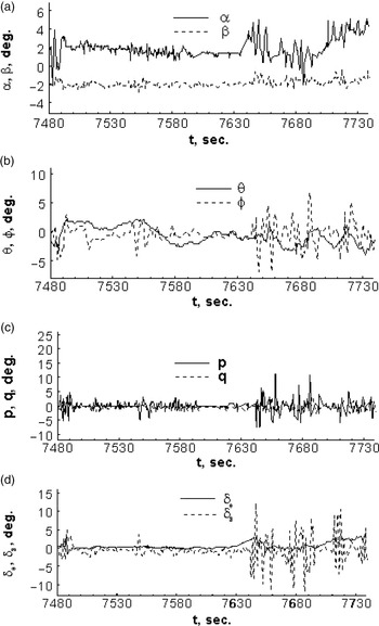
Figure 6 presents the variations of dynamic characteristics and control variables. The variation ranges of
 $\alpha$
are 4.2deg. to −2.6deg. in the first turbulence encounter and 5.5deg. to −2.2deg. in the second one; the mean value of
 $\beta$
is about −2deg. with the magnitude of small fluctuation, as indicated in Fig. 6(a). The time history of pitch angle (
 $ \theta$
) and roll angle (
 $\phi$
) is shown in Fig. 6(b). The pitch angle (
 $ \theta$
) does not vary as much as the angle-of-attack (
 $\alpha$
), reaching only 2.5deg. The variations in
 $\phi$
is large, especially during the second turbulence encounter. The magnitudes of pitch rate (q) and roll rate (p) are shown in Fig. 6(c); the variation of p is larger than that of q. The yaw rate is not shown because it is small throughout.
The variations of dynamic characteristics and control variables in severe clear-air turbulence.

The flight data recorder indicated the autopilot was deactivated from t = 7,489sec to t = 7,493sec, for 4seconds. It is of interest to examine the pilot’s response in operations after the autopilot being tripped off. The time history of
 $\delta_{e}$
and
 $\delta_{a}$
is shown in Fig. 6(d). The magnitude of
 $\delta_{e}$
becomes positive to keep pitch down in descending flight. The variation of
 $\delta_{a}$
in the second turbulence encounter is larger than that of the 1st one. While the roll angle (
 $\phi$
) is changing fast in the negative direction right before t = 7,643sec,
 $\delta_{a}$
is increasingly more positive, reaching +13deg at t = 7,645sec, as shown in Fig. 6(d). On the other hand, opposite changes occur around t = 7,646sec. The
 $\delta_{r}$
is not shown because it is small throughout.
Both the pitch and roll rates are significant in severe atmospheric turbulence, especially the latter. In normal flight conditions, pitch and roll rates are typically small, in particular at transonic speeds, to avoid nonlinear aerodynamic effects. The autopilot was tripped off in severe atmospheric turbulence. The pitch angle and roll angle are the only cues to the pilots in making the control decision.
The dynamic aerodynamic effects in the first turbulence encountered will be centralised after this section due to the following three reason:
-
1) The large vertical acceleration
-
2) The large drop-off heigh
-
3) The autopilot was deactivated from t = 7,489sec to t = 7,493sec, for 4 seconds
3.3 Analysis of model predictions
The accuracy of the established flight control models and sub-models for this transport through fuzzy-logic algorithm is estimated by the sum of squared errors (SSE) and the square of multiple correlation coefficients (R 2 ) [Reference Lan and Chang16]. The predicted data by models and sub-models to compare with those of flight data in descending phase in the period of t = 7,475–7,500sec. is presented in Figs. 7–12. All the predicted data by the final models have good match with the flight data.
Predicted rudder angle (
 $\delta_{r}$
) in descending phase based on FDR data.

Predicted lateral acceleration (
 $a_{y}$
) in descending phase based on FDR data.

Predicted aileron angle (
 $\delta_{a}$
) in descending phase based on FDR data.

Predicted elevator angles (
 ${\delta _e}$
) in descending phase based on FDR data.

Predicted angle-of-attack (
 $\alpha$
) in descending phase based on FDR data.

Predicted vertical accelerations (
 $a_{z}$
) in descending phase based on FDR data.

3.4 Mitigation of abrupt change in attitude
To improve the understanding of non-linear dynamic aerodynamic responses, Chang, et al. applied eigenvalue approach to evaluate dynamic stability characteristics and turbulence hazard levels through a six-DOF flight simulation for a specific accident event of severe turbulence encounter [Reference Chang, Ye, Lan and Guan1, Reference Chang5]. The results of flight simulation showed that some motion modes of a specific accident event were in unstable conditions during sudden plunging motion. The above study is much helpful to understand the effects of severe clear-air turbulence on instability characteristics. The mitigation concepts of abrupt changes in attitude with the corresponding gravitational accelerations will have a detail description as follows.
3.4.1 Mitigation of abrupt change in lateral-directional attitude
It is well known that horizontal wind shear, or varying crosswind, would induce rolling motion [Reference Lan and Chang16]. The rolling motion in horizontal wind shear corresponding to aileron deflections in the period of 7,482–7,494sec is presented in Fig. 13.
Rolling motion in horizontal wind shear corresponding to aileron deflections.

The magnitude of roll angles (
 $\phi$
) only has small variations during the time span from t = 7,482sec to 7,494sec., as shown in Fig. 13(a) due to the magnitude of crosswind is very small (Fig. 12(a)). The corresponding aileron input (
 $\delta_{a}$
) in Fig. 13(b) is effective to control the small variation of roll angles (
 $\phi$
) before the plunging motion. The roll control power derivatives should be positive in the normal case, referred to the effectiveness criteria in Table 6. Some parts of
 $C_{l \delta a}$
are negative during the autopilot tripped off as shown in Fig. 13(c), it implies that controllability is not good due to the aerodynamic lag effect in plunging motion.
The yaw and roll motions have some variations due to the crosswind effects as shown in Figs. 5(c) and 13(a). The largest drop-off height reaches 57.3m in the time span between t = 7,484–7,486sec, as shown in Table 7. The variations of time rates of heading angles (
 $\dot \psi $
) and roll angle (
 $\dot \varphi $
) are evaluated at the instantaneous conditions, instead of the trim conditions of the traditional approach.
The variations of operational actions of rudder (
 $\delta_{r}$
), time rates of heading angles (
 $\dot \psi $
) and lateral acceleration (
 $a_{y}$
) are large in the period of t = 7,484–7,493sec., as shown by the solid lines in Figs. 14–16, respectively.
Original and improved rudder control (
 $\delta_{r}$
).

Original and improved time rates of heading angles (
 $\dot \psi $
).

Original and improved lateral acceleration (
 $a_{y}$
).

The large variations of
 $\dot \psi $
and
 $a_{y}$
in the period of t = 7,484–7,493sec are reduced, as shown by dotted lines in Figs. 15 and 16, respectively, after the improvements of rudder operations through flight simulations of dynamic inversion process in Fig. 14. There are significant differences between the original time rates of heading angles and improved one in Fig. 15.
The original roll angle () is represented by the solid line in Fig. 17 The value of
 $\phi$
changes from negative to positive at t = 7,490sec; the values are negative in the period of t = 7,482–7,490sec; the variations of
 $\phi$
are changed rapidly in the time period of t = 7,489–7,493sec in the period of autopilot tripped off. The sensitivity analysis of
 $\phi$
variations is presented in Fig. 18; the original time rate of roll angle (
 $\dot \varphi $
) is represented by the solid line. The responses of aileron control against variations are shown in Fig. 19; the original time rate of
 $\delta_{a}$
is represented by the solid line. The highest
 $\delta_{a}$
value is around 6deg. at t = 7,487sec. The variations of original and
 $\dot \varphi $
are reduced, as shown by dotted lines in Figs 17 and 18, after the improvements of aileron control through flight simulations of dynamic inversion process. There are some differences between the original and improved aileron controls in Fig. 19.
Original and improved roll angle (
 $\phi$
).

Original and improved time rate of roll angle (
 $\dot \varphi $
).

Original and improved aileron control (
 $\delta_{a}$
).

3.4.2 Mitigation of abrupt change in longitudinal attitude
Figures 20–24 present the original and improved vertical accelerations, angles of attack, pitch angles, time rate of pitch angles, and elevator angles; the solid and dotted lines represent the original flight data and results of flight control strategy, respectively. The vertical acceleration variation of original flight data is presented in Fig. 20, showing the highest
 $a_{z}$
being 2.07g around t = 7,485sec and the lowest being −1.05g. After the applications of improved control strategy, the plunging downward with vertical accelerations are reduced from 2.07g to 1.60g in the period of t = 7,484–7,485sec and plunging upward with vertical accelerations are increased from −1.05 to 0.97 as shown by the dotted lines in Fig. 20. The applications of flight control strategy have obvious benefits.
Original and improved vertical accelerations (
 $a_{z}$
).

Original and improved angle-of-attack (
 $\alpha$
).

Original and improved pitch angle (
 $\theta $
).

Original and improved time rate of pitch angle (
 $\dot \theta $
).

Original and improved elevator angles (
 ${\delta _e}$
).

Figure 21 shows that variations of
 $\alpha$
is approximately in phase with
 $a_{z}$
. The largest and lowest angles of attack are 4.2deg. and −1.8deg., respectively; the time history of its angle-of-attack is increased first and reduced afterward. The conditions of sudden increase and abrupt decrease in angles of attack are mitigated after the applications of flight control strategy; the largest angle-of-attack 4.2deg. is reduced to 1.6deg. and the lowest angles of attack −1.8deg. is increased to 0.26deg. as shown by the dotted lines in Fig. 21.
The time history of pitch angles is decreased first and then increased to correspond with the angle-of-attack, as shown in Fig. 22. The variations of time rate of pitch angle for are shown in Fig. 23. The improved
 $\theta $
and
 $\dot \theta $
are reduced to compare with those of original data, as shown by dotted lines in Figs. 11 and 23, after the improvements of pitch control through flight simulations of dynamic inversion process. There are some differences between the original and improved pitch control; the dotted line represents improved pitch control.
The elevator angles before t = 7,475sec were basically no elevator activity. In the period of t = 7,484–7,500sec, almost all the values of elevator are negative, except the values of elevators are positive in the period of t = 7,487–7,488sec. Positive values of elevator represent nose-down elevator activities; the magnitudes of angles of attack and pitch angles should be decreased or negative. The variations of original elevator angles are reduced, as shown by dotted lines in Fig. 24, after the improvements of elevator control through flight simulations of dynamic inversion process. There are some differences between the original and improved elevator control.
4.0 Concluding remarks
The main objective in this paper was to present a new concept of the loss of control prevention to mitigate the hazards for transport aircraft in severe clear-air turbulence. This paper employed flight data mining and fuzzy-logic modeling techniques to establish flight controllability models based on the datasets from the FDR. The flight controllability models with the function of nonlinear dynamic inversion were employed to provide flight control strategy through flight simulations. This transport aircraft encountered severe clear-air turbulence twice during the descending phase. The simulated results of the flight controllability models determined the flight control strategy of rudder, aileron and elevator controls. The flight control strategy in avoidance of injuries for passengers and cabin crews during sudden plunging motion could provide the training program of loss of control prevention for the airlines. The applications of modeling and its flight simulation were concluded as follows:
-
1) The predicted results showed that the final models of flight controllability could not only produce relatively accurate flight control angles, but also generate smooth dynamic curves with the required independent variables to provide the desired dynamic analyses.
-
2) The simulated results demonstrated that the application of nonlinear dynamical inversion reduces the angles of the flight-control variables while reducing the time rate of change of angles and then increasing the damping of the control variables. The decision making of flight control strategy could be initiated through the simulations of dynamic inversion process.
-
3) Since the sudden plunging motion with the abrupt change in gravitational acceleration (g) and angles of attack affects the flight safety the most. During the first clear-air turbulence encounters, the plunging downward with vertical accelerations were reduced from 2.07g to 1.60g and plunging upward were increased from −1.05 to 0.97; the largest angle-of-attack 4.2deg. was reduced to1.6deg. and the lowest angles of attack −1.8deg. was increased to 0.26deg., after the applications of flight control strategy. The applications in loss of control prevention have obvious benefits. To mitigate the larger variations of vertical acceleration would be considered as our future research.
The analytical results could provide the mitigation concepts and promote the understanding of dynamic responses of the transport aircraft in severe clear-air turbulence. The constructions of situation awareness and expert strategy knowledge bases require more study cases; these parts will be the future tasks in our research team. The present concept is an innovation to improve aviation safety and operational efficiency for the airlines. It is expected to provide a training course for loss of control in-flight program to the airlines after this paper being published.
Data and information availability statement
The flight data of FDR from the specific aviation accident to support the present study is restricted to deliver to the third party. The flight number, name of airlines and aircraft manufacture are not publicly available without permission.
Acknowledgments
This work was supported in part by the following grants with three different sources:
-
1) Joint Funds project of the National Natural Science Foundation of China (grant no. U1733203), the special key projects of technological innovation and application development of Chongqing (grant no. cstc2019jscx-fxydX0036)
-
2) The scientific research project of CQJTU (grant no. 19JDKJC-A012)
-
3) China Postdoctoral Science Foundation (grant no. 2020M671385)