





1. Introduction
The numerical investigation of turbulent flows in straight ducts with non-circular cross-section is of great interest for many engineering applications, such as turbomachinery, heat exchangers and nuclear reactors. In rectangular ducts, the flow features two inhomogeneous directions, and exhibits secondary motions in the cross-stream plane arising from turbulence, first studied by Prandtl (Reference Pope1926, Reference Prandtl1927) and Nikuradse (Reference Nagib and Chauhan1930). These secondary flows have an intensity that is a small fraction of the mean stream velocity, but their effect on wall shear stress and heat transfer along the perimeter is significant because of their persistence (Leutheusser Reference Launder and Ying1963; Gessner & Jones Reference Gavrilakis1965; Modesti et al. Reference Modesti and Pirozzoli2018). Secondary motions in ducts are associated with non-zero streamwise vorticity, which may result from skewing of existing spanwise vorticity, as in curved ducts, or from Reynolds stress gradients induced by non-circular cross-sections. Prandtl accordingly distinguished secondary motions of the first and second kind. Secondary motions of the second kind are often studied in square-duct flow owing to its simple geometry, which is convenient for testing and developing turbulence models. In this case, the mean transverse flow consists of pairs of counter-rotating streamwise vortices in each quadrant, transporting high-momentum fluid from the core towards the corners along the bisectors, and returning low-momentum fluid to the duct centre along the wall bisectors.
Several experimental campaigns have provided quantitative measurements and insight into the mechanisms of streamwise vorticity production and its dependence on Reynolds number (Brundrett & Baines Reference Brundrett and Baines1964; Gessner & Jones Reference Gavrilakis1965; Demuren & Rodi Reference Demuren and Rodi1984). Based on such data, those authors concluded that secondary motions strongly influence the streamwise vorticity balance, likely governed by Reynolds stress gradients and convection from secondary motions. More recently, Nagata et al. (Reference Monkewitz2011) showed from experiments on flows over right-angled plates that the intensity of secondary motions at high Reynolds number should scale with the turbulence intensity, represented in ducts by the friction velocity.
Direct numerical simulations (DNS) have also proven effective for studying turbulence in complex ducts and clarifying the nature of secondary motions. The first DNS of square-duct flow were carried out by Gavrilakis (Reference van Driest1992) and Huser & Biringen (Reference Hu, Hayat and Park1993). The former described the mean flow in the cross-section and turbulence statistics along the wall bisector at low Reynolds number. The latter produced a database for fully developed turbulent square-duct flow, highlighting the influence of the corners on turbulence statistics and on the origin of secondary motions of the second kind. Uhlmann et al. (Reference Spalart, Garbaruk and Stabnikov2007) and Pinelli et al. (Reference Nouri, Umur and Whitelaw2010) extended the DNS to a range of low Reynolds numbers, reporting that longer integration times are required to achieve statistical convergence as Reynolds number increases. Pirozzoli et al. (Reference Pirozzoli2018) performed DNS of turbulent flow in a square duct over a wide range of moderate Reynolds numbers, and found that the intensity of secondary motions scales more closely with the bulk velocity than with the friction velocity. They distinguished two types of circulation: a corner circulation, with typical size of the viscous length scale, and a core circulation, with size of the duct half-side. The corner circulation, associated with higher vorticity, becomes more confined near the corners as Reynolds number increases; the core circulation is weaker, but carries most of the cross-stream flow, influencing a large portion of the duct. They also showed that the logarithmic law of the wall holds with high accuracy from the near-wall region up to the corner bisector, suggesting strong universality of wall turbulence. This finding is consistent with earlier scattered experiments (e.g. Jonsson & Sparrow Reference Huser and Biringen1966; Cain & Duffy Reference Cain and Duffy1971; Nouri et al. Reference Nikuradse1993), with studies of rectangular ducts (Vinuesa et al. Reference Vinuesa, Noorani, Lozano-Durán, Khoury, Schlatter, Fischer and Nagib2014), and with hexagonal ducts (Marin et al. Reference Madabhushi and Vanka2016).
A formal theoretical framework for turbulent flow in straight ducts with arbitrary cross-section was developed by Spalart et al. (Reference Smagorinsky2018). Extending classical inner–outer matching arguments, and assuming the local friction velocity as the relevant scale, they deduced the continued validity of the logarithmic law, and predicted that wall friction should tend to become uniform around the duct, except near corners, in the limit
 $\textit{Re} \to \infty$
. Testing these theoretical predictions in the infinite-Reynolds-number limit requires simulations at Reynolds numbers considerably higher than those reached so far. Despite increasing computational power, DNS remain prohibitively expensive, and are confined to low and moderate Reynolds numbers. Large-eddy simulations (LES) provide a viable alternative, as only the large scales are resolved, with subgrid scales modelled, reducing the computational cost. However, wall-resolved LES still require grids fine enough to capture turbulence in the buffer layer, which limits the maximum Reynolds number achievable. A more affordable approach is wall-modelled LES (WMLES), in which the near-wall region is replaced with a wall model that supplies boundary conditions (Larsson et al. Reference Kim and Moin2016). Such WMLES have previously been applied to canonical flows such as channel flow (Chung & Pullin Reference Chung and Pullin2009) and Couette flow (Cheng et al. Reference Cheng, Pullin and Samtaney2022) to infer their asymptotic high-Reynolds-number behaviour. A key result, in accordance with the observations of Pullin et al. (Reference Prandtl2013), is that several simple flows are characterised by an asymptotic state in the high-Reynolds-number limit, in which turbulence intensity diminishes, and turbulence effects like secondary motions are progressively confined near the walls. As evidence of this, Cheng et al. (Reference Cheng, Pullin and Samtaney2022) and Pirozzoli (Reference Pinelli, Uhlmann, Sekimoto and Kawahara2024) reported that the streamwise turbulence intensity exhibits an asymptotic plateau for
 $\textit{Re}_\tau \to \infty$
, when scaled with the friction velocity. The WMLES have also been successfully applied to more complex flows, such as bent ducts (Cho et al. Reference Cho, Lozano-Durán, Moin and Park2021; Hu et al. Reference Harlow and Welch2023), and have provided valuable numerical evidence regarding the appropriate scaling laws for high-Reynolds-number wall-bounded turbulent flows (Cheng & Samtaney Reference Cheng and Samtaney2014).
In this paper, we employ WMLES to study turbulent flow in a square duct over a very wide range of Reynolds numbers, with the main goals of: (i) qualifying the use of WMLES to study internal flows in ducts with complex cross-section; (ii) inferring the asymptotic properties of flow in square ducts, particularly the mean friction coefficient, the friction distribution along the walls, and the intensity of the secondary motions. Comparison with DNS data at moderate Reynolds numbers is instrumental in establishing the reliability of our predictions. The paper is organised as follows. The simulation set-up is described in § 2. Results are presented in § 3, focusing on the mean velocity field, wall friction, and secondary flows. Concluding remarks are given in § 4.
2. Numerical method
We solve the filtered incompressible Navier–Stokes equations:
 \begin{equation} \frac {\partial \overline {u}_{\!j}}{\partial x_{\!j}} = 0, \end{equation}
 \begin{equation} \frac {\partial \overline {u}_i}{\partial t} + \frac {\partial \overline {u}_i \overline {u}_{\!j}}{\partial x_{\!j}} = -\frac {1}{\rho } \frac {\partial \overline {p}}{\partial x_i} + \nu \frac {\partial ^2 \overline {u}_i}{\partial x_{\!j}\, \partial x_{\!j}} - \frac {\partial \tau _{ij}}{\partial x_{\!j}} + \varPi \delta _{i1}, \end{equation}
where
 $\overline {u}_i$
is the filtered velocity,
 $\rho$
is the fluid density,
 $\overline {p}$
is the filtered pressure, and
 $\nu$
is the kinematic viscosity. The mass flow rate is kept constant in time through the addition of a spatially uniform, time-varying body force
 $\varPi$
. The subgrid-scale stress tensor is defined as
 $\tau _{ij} = \overline {u_i u_{\!j}} - \overline {u}_i \overline {u}_{\!j}$
. Its isotropic part is absorbed into a modified pressure,
 $\overline {p} \gets \overline {p} + ({1}/{3}) \rho \tau _{kk}$
, and the deviatoric part is modelled with the Boussinesq assumption:
 \begin{equation} \tau _{ij} - \frac {1}{3} \tau _{kk} \delta _{ij} = -2 \nu _t \overline {S}_{ij}, \end{equation}
where
 $\delta _{ij}$
is the Kronecker delta,
 $\overline {S}_{ij}=(1/2) ( \partial \overline {u}_i / \partial x_{\!j} + \partial \overline {u}_{\!j} / \partial x_i )$
is the filtered strain-rate tensor, and
 $\nu _t$
is the turbulent viscosity.
For closure, we adopt the classical Smagorinsky model (Smagorinsky Reference Schlichting and Gersten1963) with near-wall damping. With
 $\overline {\mathcal{S}} = (2 \overline {S}_{ij} \overline {S}_{ij} )^{1/2}$
, the subgrid-scale eddy viscosity is
 \begin{equation} \nu _t = \left ( C_s \varDelta\, D(y) \right )^2\, \overline {\mathcal{S}}, \end{equation}
where
 $C_s$
is a model constant,
 $\varDelta$
is the filter width, and
 $D(y)$
is the near-wall damping function, with
 $y$
the distance from the closest wall. The van Driest damping function (van Driest Reference Uhlmann, Pinelli, Kawahara and Sekimoto1956) is used, i.e.
 $D(y) = 1 - {\rm e}^{ -y^*/25 }$
, where
 $\ast$
denotes normalisation by global wall units. The optimal value of the model constant
 $C_s$
depends significantly on the flow features. Lilly (Reference Leutheusser1967) showed that for isotropic turbulence, with spatial resolution within the inertial subrange,
 $C_s \approx 0.17$
, whereas Deardorff (Reference Deardorff1970) suggested
 $C_s \approx 0.1$
for wall-bounded turbulent shear flows. Accordingly, we set
 $C_s = 0.11$
.
Use of a wall model effectively avoids resolving at least part of the inner-layer turbulence, thus allowing huge computational savings. Standard wall models (Kawai & Larsson Reference Jonsson and Sparrow2012; Larsson et al. Reference Kim and Moin2016) use the wall-parallel velocity at a given distance to estimate the wall shear stress, replacing the no-slip condition. Here, we adopt the logarithmic wall law
 \begin{equation} \frac {U_{wm}}{u_{\tau }} = \frac {1}{\kappa } \log \left ( \frac {u_{\tau } h_{wm}}{\nu } \right ) + B, \end{equation}
with
 $\kappa = 0.41$
and
 $B = 5.2$
(Pope Reference Pirozzoli, Romero, Fatica, Verzicco and Orlandi2000), where
 $\nu$
is the kinematic viscosity,
 $h_{wm}$
is the distance of the exchange location from the nearest wall,
 $U_{wm}$
is the corresponding wall-parallel velocity magnitude, and
 $u_\tau =(\tau _w/\rho )^{1/2}$
is the local friction velocity, with
 $\tau _w$
the local wall shear stress. Equation (2.5) is formally valid in the mean sense for equilibrium flows, yet it has proven reliable also when applied in the instantaneous sense and in non-equilibrium flows (Bermejo-Moreno et al. Reference Bermejo-Moreno, Campo, Larsson, Bodart, Helmer and Eaton2014; Larsson et al. Reference Kim and Moin2016). Its established validity in square ducts (Pirozzoli et al. Reference Pirozzoli2018) further supports its use here. In our implementation, the instantaneous wall-parallel velocity components are first linearly interpolated in the wall-normal direction to the exchange location, where
 \begin{align} U_{wm}=\left (u_{wm}^2+w_{wm}^2\right )^{1/2}. \end{align}
Here,
 $u_{wm}$
and
 $w_{wm}$
denote the interpolated streamwise and transverse velocity components, respectively. The local friction velocity is then obtained from (2.5) using a Newton–Raphson iterative procedure. Assuming that the wall shear stress vector is aligned with the wall-parallel velocity at the exchange location, its magnitude is evaluated as
 $\tau _w=\rho u_\tau ^2$
, and its components are computed as
 \begin{align} {\tau _w}_x=\tau _w\frac {u_{wm}}{U_{wm}}, \quad {\tau _w}_z=\tau _w\frac {w_{wm}}{U_{wm}}. \end{align}
The resulting stress distribution is imposed as a Neumann boundary condition for the wall-parallel velocity components, namely
 \begin{equation} {\tau _w}_x= \rho \,\nu \left . \frac {\partial \overline {u}}{\partial y} \right |_{y=0}, \quad {\tau _w}_z= \rho \,\nu \left . \frac {\partial \overline {w}}{\partial y} \right |_{y=0}, \qquad \end{equation}
where
 $y$
denotes the local wall-normal coordinate. The impermeability condition is enforced for the wall-normal velocity component. Equation (2.8) is applied locally and instantaneously to the filtered wall-parallel velocity field. The wall-normal derivatives are evaluated by linearly extrapolating the velocity field to the ghost points, and subsequently applying second-order central differencing. Periodic boundary conditions are applied along the streamwise direction, and a uniform body force is imposed to maintain constant mass flux. The simulations use the CaLES solver (Costa Reference Costa2018; Xiao et al. Reference Xiao, Ceci, Costa, Larsson and Pirozzoli2025), based on a fractional-step method (Kim & Moin Reference Kawai and Larsson1985). Time integration employs a low-storage, three-step Runge–Kutta scheme (Wray Reference Wray1990), and spatial discretisation uses second-order finite differences on staggered grids (Harlow & Welch Reference De Graaff and Eaton1965). Further implementation details, especially on the subgrid-scale and wall-stress models, are available in the original references.
The computational domain is aligned with the streamwise
 $(x)$
and transverse
 $(y,z)$
directions, with dimensions
 $L_x = 12.8 \delta$
,
 $L_{\!y} = 2 \delta$
and
 $L_z = 2 \delta$
, where
 $\delta$
is the half-side length. All simulations use a uniform grid of
 $(512 \times 128 \times 128)$
points in
 $(x,y,z)$
. The spacings are
 $\Delta x/\delta = 0.025$
,
 $\Delta y/\delta = 0.016$
and
 $\Delta z/\delta = 0.016$
, slightly finer than the guidelines of Larsson et al. (Reference Kim and Moin2016) for canonical flows. The same grid is used at all Reynolds numbers, consistent with the spirit of WMLES. The exchange point is placed at
 $h_{wm} = 0.1 \delta$
, giving six grid points below it. Grid parameters were chosen through a convergence study at moderate Reynolds number, using DNS as reference. Quantitative results were only weakly sensitive to the precise grid choice.
We consider six bulk Reynolds numbers, defined as
 $\textit{Re}_b = 2 u_b \delta / \nu$
, with
 $u_b$
the bulk velocity. The two lowest values (
 $\textit{Re}_b=40\,000$
,
 $84\,000$
) correspond to the reference DNS of Pirozzoli et al. (Reference Pirozzoli2018) and Modesti & Pirozzoli (Reference Marin, Vinuesa, Obabko and Schlatter2022). Here and throughout, the superscript
 $*$
denotes quantities scaled with the perimeter-averaged friction, namely
 $\tau ^*_w = \delta \langle \varPi \rangle /2$
, where
 $\langle \varPi \rangle$
is the time average of the body force
 $\varPi$
(see (2.2)). Resulting velocity and length scales are, respectively,
 $u^*_{\tau }=(\tau ^*_w/\rho )^{1/2}$
and
 $\delta _v^*=\nu /u^*_{\tau }$
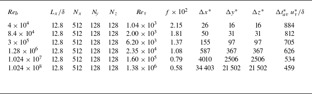
. Table 1 lists the main flow parameters, including the friction Reynolds number
 $\textit{Re}_\tau =u^*_\tau \delta /\nu$
, the friction factor
 $f = 8 \tau ^*_w / (\rho u_b^2)$
, and the grid spacings in global wall units
 $(\Delta x^*,\Delta y^*,\Delta z^*)$
. The table also reports the effective averaging intervals, defined to include the streamwise domain length (Vinuesa et al. Reference Vinuesa, Prus, Schlatter and Nagib2016), namely
 $\Delta t_{av}^* = \Delta t_{av} L_x /(6 \delta )$
, expressed in eddy-turnover times,
 $\delta /u_\tau ^*$
. For reference, Pirozzoli et al. (Reference Pirozzoli2018) used
 $\Delta t_{av}^* = 531\,\delta /u_\tau ^*$
for DNS at
 $\textit{Re}_b = 40\,000$
. These integration times are much longer than for plane channel flow, and are indeed required in order to achieve statistical convergence because of the long time scales associated with the secondary motions. The flow is initialised with a uniform velocity plus random disturbances, and the first
 $\mathcal{O}(200)$
time units were discarded from the statistical analysis to minimise the effect of initial transients. In the following, the mean velocity components, averaged both in the streamwise homogeneous direction and in time, are denoted with
 $U,V,W$
. Referring to the bottom duct wall, they indicate the streamwise, wall-normal and transverse velocity components.
Flow parameters for WMLES of square-duct turbulence:
 $\textit{Re}_b = 2 u_b \delta / \nu$
is the bulk Reynolds number,
 $L_x$
is the streamwise domain length,
 $\delta$
is the duct half-side length,
 $N_x$
,
 $N_{\!y}$
and
 $N_z$
are the numbers of grid points in each direction,
 $\textit{Re}_\tau = u_\tau ^* \delta / \nu$
is the friction Reynolds number, and
 $f = 8 \tau _w^* / (\rho u_b^2)$
is the friction factor. The quantities
 $\Delta x^*, \Delta y^*, \Delta z^*$
denote grid spacings in global wall units, and
 $\Delta t_{av}^*\, u_\tau ^* / \delta$
is the averaging window expressed in eddy-turnover times
 $\delta /u_\tau ^*$
.

Table 1. Long description
The table presents flow parameters for WMLES of square-duct turbulence. It includes six bulk Reynolds numbers and various flow parameters. The columns are as follows: Re_b (bulk Reynolds number), L_x/δ (streamwise domain length), N_x (number of grid points in the streamwise direction), N_y (number of grid points in the wall-normal direction), N_z (number of grid points in the transverse direction), Re_τ (friction Reynolds number), f * x 10^2 (friction factor), Δx* (grid spacing in the streamwise direction), Δy* (grid spacing in the wall-normal direction), Δz* (grid spacing in the transverse direction), and Δt^*+_av u_τ^*/δ (averaging window expressed in eddy-turnover times). The table lists the following data: Row 1: Re_b, 4 x 10^4; L_x/δ, 12.8; N_x, 512; N_y, 128; N_z, 128; Re_τ, 1.04 x 10^3; f * x 10^2, 2.15; Δx*, 26; Δy*, 16; Δz*, 16; Δt^+_avg u^+_τ/δ, 884. Row 2: Re_b, 8.4 x 10^4; L_x/δ, 12.8; N_x, 512; N_y, 128; N_z, 128; Re_τ, 2.00 x 10^3; f * x 10^2, 1.81; Δx*, 50; Δy*, 31; Δz*, 31; Δt^+_avg u^+_τ/δ, 812. Row 3: Re_b, 3 x 10^5; L_x/δ, 12.8; N_x, 512; N_y, 128; N_z, 128; Re_τ, 6.20 x 10^3; f * x 10^2, 1.37; Δx*, 155; Δy*, 97; Δz*, 97; Δt^+_avg u^+_τ/δ, 705. Row 4: Re_b, 1.28 x 10^6; L_x/δ, 12.8; N_x, 512; N_y, 128; N_z, 128; Re_τ, 2.35 x 10^4; f * x 10^2, 1.08; Δx*, 587; Δy*, 367; Δz*, 367; Δt^+_avg u^+_τ/δ, 626. Row 5: Re_b, 1.024 x 10^7; L_x/δ, 12.8; N_x, 512; N_y, 128; N_z, 128; Re_τ, 1.60 x 10^5; f * x 10^2, 0.79; Δx*, 4010; Δy*, 2506; Δz*, 2506; Δt^+_avg u^+_τ/δ, 534. Row 6: Re_b, 1.024 x 10^8; L_x/δ, 12.8; N_x, 512; N_y, 128; N_z, 128; Re_τ, 1.38 x 10^6; f * x 10^2, 0.58; Δx*, 34403; Δy*, 21502; Δz*, 21502; Δt^+_avg u^+_τ/δ, 459.
3. Results
3.1. Mean flow
Contours of the mean streamwise velocity in the duct cross-section are shown in figure 1. As observed in DNS (Pirozzoli et al. Reference Pirozzoli2018), the mean velocity isolines bulge towards the corners, reflecting the convection of momentum by the secondary motions from the high-momentum duct core to the low-momentum corners along the bisectors. Consequently, flattening of velocity profiles and the increase of wall-normal gradients as a result of enhanced turbulent mixing is observed (Madabhushi & Vanka Reference Lilly1991). Agreement with DNS data (Pirozzoli et al. Reference Pirozzoli2018; Modesti & Pirozzoli Reference Marin, Vinuesa, Obabko and Schlatter2022) at low
 $\textit{Re}$
is good and appears to improve with increasing
 $\textit{Re}$
. A minor discrepancy is that WMLES slightly underestimate the velocity near the corner bisectors. Overall, the flow structure appears essentially universal at Reynolds numbers beyond the current reach of DNS. As expected, with increasing
 $\textit{Re}_b$
, the velocity isolines cluster near the duct walls and become sparser in the bulk.
Contours of mean streamwise velocity (
 ${U}/u_b$
) obtained with WMLES (coloured lines) and DNS (black lines). The dashed line denotes the position of the exchange point along the duct perimeter, and the vertical segment denotes the duct wall bisector. The solid black line in (a,b) corresponds to the DNS data of Pirozzoli et al. (Reference Pirozzoli2018) and Modesti & Pirozzoli (Reference Marin, Vinuesa, Obabko and Schlatter2022).

Contours of mean transverse velocity (
 ${W}/u_b$
), obtained with WMLES (coloured lines) and DNS (black lines). The dashed line denotes the position of the exchange point along the duct perimeter, and the vertical segment denotes the line
 $0\leq y/\delta \leq 1$
,
 $z/\delta = 0.5$
. The solid black line in (a,b) corresponds to the DNS data of Pirozzoli et al. (Reference Pirozzoli2018) and Modesti & Pirozzoli (Reference Marin, Vinuesa, Obabko and Schlatter2022).

Figure 2 shows contours of the mean cross-stream velocity in the
 $z$
direction. Secondary motions are strongest near the duct corners, whereas return motions occur along the wall bisectors. Good quantitative agreement with the DNS data of Pirozzoli et al. (Reference Pirozzoli2018) and Modesti & Pirozzoli (Reference Marin, Vinuesa, Obabko and Schlatter2022) is also found for this quantity. The figure indicates that at moderate Reynolds numbers, the typical intensity of secondary motions velocity components does not exceed approximately
 $2\,\%$
of the bulk velocity. Specifically, the maximum secondary-velocity magnitude (
 $(V^2+W^2)^{1/2}$
) slightly decreases from
 $2.17\,\%\,u_b$
at
 $\textit{Re}_b=40\,000$
to
 $1.22\,\%\,u_b$
at
 $\textit{Re}_b=102\,400\,000$
. These values are consistent with earlier computations of Madabhushi & Vanka (Reference Lilly1991) at
 $\textit{Re}_b = 5810$
, and measurements of Brundrett & Baines (Reference Brundrett and Baines1964) at
 $\textit{Re}_b = 83\,000$
, who reported maximum secondary velocities of approximately
 $2.5\,\%$
and
 $2.2\,\%$
of
 $u_b$
, respectively. The mean transverse velocity
 $W$
is plotted along the line
 $0 \le y/\delta \le 1$
at
 $z/\delta = 0.5$
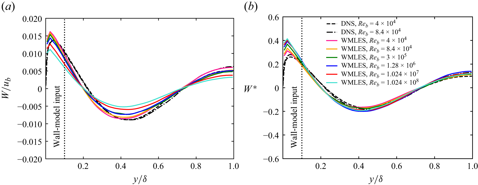
, corresponding to the vertical segment indicated in figure 2. A comparison with DNS data is shown in figure 3, where good overall agreement is observed above the wall-model exchange location. Consistent with the experimental findings of Brundrett & Baines (Reference Brundrett and Baines1964), Gessner & Jones (Reference Gavrilakis1965) and Launder & Ying (Reference Larsson, Kawai, Bodart and Bermejo-Moreno1972), normalisation with the bulk velocity yields a progressive reduction of the secondary motion intensity with increasing Reynolds number, whereas scaling with the global friction velocity yields approximate universality of the profiles.
The shape of the secondary motions is considered in figure 4, which displays isolines of the cross-stream streamfunction. Regardless of Reynolds number, and in agreement with previous studies, eight counter-rotating triangular rollers are observed. Their sense of rotation conveys high-speed fluid from the duct core towards the corners, with return motions along the wall bisectors. Quantitative agreement with the DNS data of Pirozzoli et al. (Reference Pirozzoli2018) and Modesti & Pirozzoli (Reference Marin, Vinuesa, Obabko and Schlatter2022) is good, and again a gradual weakening of the secondary eddies is evident with increasing Reynolds number. Overall, this analysis confirms the predictive accuracy of WMLES in resolving the general organisation of the flow.
3.2. Statistics along the wall bisector
Velocity statistics were collected along the bisector of the lower wall (i.e. the
 $z/\delta =1$
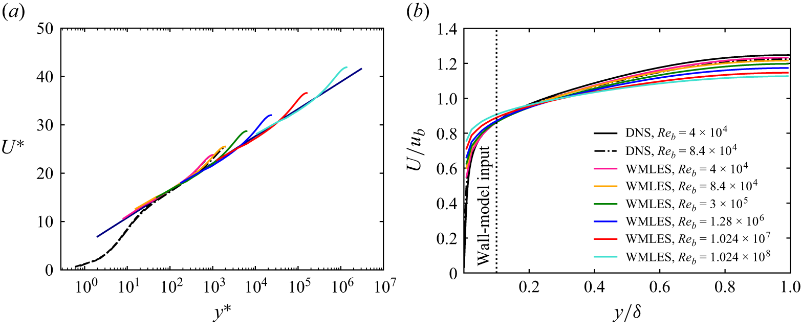
traverse from the wall to the duct centreline, represented as the vertical segment in figure 1). The inner-scaled mean velocity profiles are shown in figure 5(a), where
 $U^*={U}/u_{\tau }^*$
is plotted against
 $y^*=y/\delta ^*_\nu$
. As expected based on the grid resolution, the inner part of the wall layer is not resolved in the WMLES, even at Reynolds numbers accessible to DNS. Still, very good agreement with the DNS data is found starting from the logarithmic layer and into the wake region. Specifically, all velocity profiles follow the target logarithmic wall law
 \begin{equation} u_{\mathit{log}}^*=\log (y^*)/\kappa +B \end{equation}
over an increasing interval of inner-scaled wall distances, before deviating from it as the duct centreline is approached, thus corroborating the validity of the logarithmic-law scaling in the overlap region.
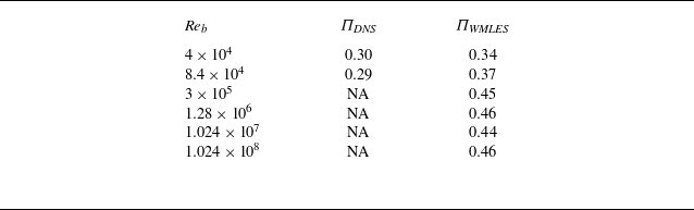
Deviations from the standard logarithmic profile are quantified in terms of the Coles wake-strength parameter (Coles Reference Coles1956)
 \begin{equation} \varPi = \frac {2}{\kappa }\big ( u_{\textit{CL}}^* - u_\mathit{log}^* \big ). \end{equation}
The resulting values are reported in table 2. Discrepancies of approximately
 $20\,\%$
with respect to DNS are observed, primarily associated with the imperfect prediction of the friction coefficient. Extrapolation to higher Reynolds numbers indicates that after an initial increase,
 $\varPi$
fluctuates around an approximately constant value of
 $0.45$
. Interestingly, this behaviour closely resembles that reported for turbulent boundary layers (Nagib & Chauhan Reference Nagata, Hunt, Sakai and Wong2008).
Coles wake strength parameter for square-duct turbulence:
 $\textit{Re}_b = 2 u_b \delta / \nu$
is the bulk Reynolds number, and
 $\varPi _{\textit{DNS}}$
and
 $\varPi _{\textit{WMLES}}$
are the wake parameters computed from DNS and WMLES data, respectively.

Table 2. Long description
A table comparing wake-strength parameters for different Reynolds numbers using DNS and WMLES data. The table has three columns and six rows. The columns are labeled as follows: Re_b, Pi_DNS, and Pi_WMLES. The rows are labeled with different Reynolds numbers and their corresponding wake-strength parameters. Row 1: Re_b, 4 x 10^4; Pi_DNS, 0.30; Pi_WMLES, 0.34. Row 2: Re_b, 8.4 x 10^4; Pi_DNS, 0.29; Pi_WMLES, 0.37. Row 3: Re_b, 3 x 10^5; Pi_DNS, NA; Pi_WMLES, 0.45. Row 4: Re_b, 1.28 x 10^6; Pi_DNS, NA; Pi_WMLES, 0.46. Row 5: Re_b, 1.024 x 10^7; Pi_DNS, NA; Pi_WMLES, 0.44. Row 6: Re_b, 1.024 x 10^6; Pi_DNS, NA; Pi_WMLES, 0.46. The table shows the wake-strength parameters for different Reynolds numbers, with some values not available (NA) for higher Reynolds numbers in the DNS column.
Mean transverse velocity component along the line
 $0\leq y/\delta \leq 1$
,
 $z/\delta = 0.5$
: (a) bulk-velocity normalisation; (b) global friction velocity normalisation.

Contours of mean streamfunction over the square-duct cross-section, obtained with WMLES (coloured lines) and DNS (black lines). The dashed line denotes the position of the exchange point along the duct perimeter. The solid black line in (a,b) corresponds to the DNS data of Pirozzoli et al. (Reference Pirozzoli2018) and Modesti & Pirozzoli (Reference Marin, Vinuesa, Obabko and Schlatter2022).

Figure 4. Long description
Panel A: A heat map showing the mean streamfunction contours in a square duct for a Reynolds number of 4 times 10 to the power of 4. The x-axis is labeled z over delta, ranging from 0 to 2. The y-axis is labeled y over delta, also ranging from 0 to 2. The color scale ranges from -0.002 to 0.002, with red indicating lower values and blue indicating higher values. The contours are overlaid with black lines representing DNS data. Panel B: A heat map showing the mean streamfunction contours in a square duct for a Reynolds number of 8.4 times 10 to the power of 4. The axes and color scale are the same as in Panel A. The contours are overlaid with black lines representing DNS data. Panel C: A heat map showing the mean streamfunction contours in a square duct for a Reynolds number of 3 times 10 to the power of 5. The axes and color scale are the same as in Panel A. Panel D: A heat map showing the mean streamfunction contours in a square duct for a Reynolds number of 1.28 times 10 to the power of 6. The axes and color scale are the same as in Panel A. Panel E: A heat map showing the mean streamfunction contours in a square duct for a Reynolds number of 1.024 times 10 to the power of 7. The axes and color scale are the same as in Panel A. Panel F: A heat map showing the mean streamfunction contours in a square duct for a Reynolds number of 1.024 times 10 to the power of 8. The axes and color scale are the same as in Panel A.
Mean velocity profiles along the lower wall bisector shown in (a) global inner scaling and (b) outer scaling. The thin line in (a) denotes the reference logarithmic wall law
 $u^*=\log (y^*)/0.41+5.2$
.

Figure 5(b) presents the mean streamwise velocity profiles scaled in outer units
 $(\delta ,u_b)$
. The profiles confirm the progressive clustering of velocity isolines near the duct walls observed in figure 1: with increasing Reynolds number, the wall-bisector profiles steepen in the near-wall region, and flatten towards the centreline. A similar trend was reported by Cheng et al. (Reference Cheng, Pullin, Samtaney and Luo2023) in their WMLES of plane Couette–Poiseuille flow.
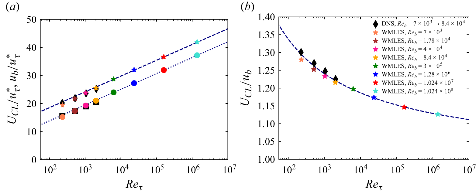
(a) Mean centreline velocity (
 $U_{\textit{CL}}^*$
, upper symbols) and bulk velocity (
 $u_b^*$
, lower symbols) in inner scaling as functions of the Reynolds number. The dashed and dotted lines denote the corresponding fits defined in (3.3). The black symbols denote DNS data of Pirozzoli et al. (Reference Pirozzoli2018) and Modesti & Pirozzoli (Reference Marin, Vinuesa, Obabko and Schlatter2022). (b) The ratio
 $U_{\textit{CL}}/u_b$
.

A more detailed assessment of the asymptotic trends of the velocity profiles is provided in figure 6, which shows the mean centreline velocity
 $U_{\textit{CL}}$
and the bulk velocity, both scaled by the global friction velocity, as functions of the friction Reynolds number (figure 6
a), together with their ratio (figure 6
b). Consistent with both theoretical predictions (Monkewitz Reference Modesti, Pirozzoli, Orlandi and Grasso2021) and DNS results (Pirozzoli et al. Reference Pirozzoli, Modesti, Orlandi and Grasso2021), the data indicate a logarithmic increase with
 $\textit{Re}_\tau$
of the form
 \begin{equation} U_{\textit{CL}}^*=\frac {1}{\kappa }\log \textit{Re}_\tau + B_{\textit{CL}}, \quad U_{b}^*=\frac {1}{\kappa }\log \textit{Re}_\tau + B, \end{equation}
with
 $\kappa =0.41$
as in the logarithmic law of the wall, and
 $B_{\textit{CL}}=7.3$
,
 $B=2.6$
. Both DNS and WMLES data for square-duct flow follow a consistent trend over the investigated Reynolds number range, with satisfactory agreement at low and moderate Reynolds numbers. As a consequence of the common logarithmic growth, the ratio shown in figure 6(b) approaches unity slowly with increasing Reynolds number. This behaviour is consistent with the trend observed in figure 5(b), and is further supported by the secondary-velocity profiles shown in figure 3. Together, these observations suggest that square-duct turbulence at finite Reynolds number may be viewed as a departure from an asymptotic plug-flow state. From this perspective, the progressive weakening of the secondary motions in outer scaling, and the evolution of the outer-scaled streamwise velocity profiles towards a flatter shape, represent complementary manifestations of the same asymptotic behaviour. This interpretation is consistent with analogous inferences made for channel flow (Pullin et al. Reference Prandtl2013).
Traverses of Reynolds stress components along the wall bisector: (a–c) resolved components of the normal stresses; (d) sum of resolved and subgrid components of the shear stress.

Figure 7. Long description
The image contains four line graphs labeled (a), (b), (c), and (d), each depicting different components of Reynolds stress along the wall bisector. Panel A: This line graph shows the resolved components of the normal stress (uu) against the normalized wall distance (y/δ). The x-axis is labeled y/δ and spans from 10^-3 to 10^0, while the y-axis is labeled (uu) and ranges from 0 to 10. Multiple lines represent different Reynolds numbers and DNS data, with a vertical dashed line indicating the wall-model input. Panel B: This line graph displays the resolved components of the normal stress (ww) against the normalized wall distance (y/δ). The x-axis is labeled y/δ and spans from 10^-3 to 10^0, while the y-axis is labeled (ww) and ranges from 0 to 3. Multiple lines represent different Reynolds numbers and DNS data, with a vertical dashed line indicating the wall-model input. Panel C: This line graph shows the resolved components of the normal stress (vv) against the normalized wall distance (y/δ). The x-axis is labeled y/δ and spans from 10^-3 to 10^0, while the y-axis is labeled (vv) and ranges from 0 to 1.4. Multiple lines represent different Reynolds numbers and DNS data, with a vertical dashed line indicating the wall-model input. Panel D: This line graph depicts the sum of resolved and subgrid components of the shear stress (uv) against the normalized wall distance (y/δ). The x-axis is labeled y/δ and spans from 10^-3 to 10^0, while the y-axis is labeled -\langle uv \rangle^* and ranges from 0 to 1.2. Multiple lines represent different Reynolds numbers and DNS data, with a vertical dashed line indicating the wall-model input. Each graph shows how the stress components vary with the wall distance for different Reynolds numbers, providing insights into the behavior of turbulent flow in straight ducts.
The wall-normal distributions of the resolved part of the diagonal Reynolds stress components are shown in figures 7(a–c). Hereafter, the angle brackets are used to denote quantities averaged along the streamwise direction and in time. All stresses are scaled by the average wall shear stress
 $\tau _w^*=\rho {u_\tau ^*}^2$
, and plotted against the outer-scaled wall-normal distance. As expected, WMLES cannot resolve the inner-layer peaks of the streamwise (
 $\langle \overline {u} \, \overline {u} \rangle$
), wall-normal (
 $\langle \overline {v} \, \overline {v} \rangle$
) and spanwise (
 $\langle \overline {w} \,\overline {w} \rangle$
) resolved stresses, because of both lack of resolution and missing subgrid contribution. The latter has been absorbed into a modified pressure and is not modelled within a Boussinesq-like closure as herein assumed (see § 2). Turbulence in WMLES is generated and subsequently dissipated in the outer layer (Larsson et al. Reference Kim and Moin2016). Hence farther than the exchange location, the streamwise stress is predicted quite accurately. The agreement is less satisfactory for the spanwise and wall-normal stresses, which are accurately predicted only for
 $y/\delta \gtrsim 0.3$
. In addition, the two lower-Reynolds-number cases exhibit behaviour distinct from that of the higher-
 $\textit{Re}$
cases in figures 7(b) and 7(c). This discrepancy may reflect limitations of the equilibrium logarithmic wall model employed here, or the use of a uniform computational grid for all Reynolds numbers, which is designed primarily to resolve the outer region of the flow. In that region, the correct decay of the spanwise and wall-normal stresses is recovered. Consistent with the WMLES framework, we do not expect accurate resolution of the near-wall region, but rather a faithful representation of the large-scale motions. Since secondary motions are a macroscopic phenomenon governed by gradients of the resolved Reynolds stresses over the entire duct cross-section, their prediction is not expected to be severely affected by near-wall inaccuracies, provided that the outer-layer stresses are correctly captured.
Figure 7(d) shows the wall-normal distribution of the turbulent shear stress, also including the subgrid-scale part, namely
 $-\langle \overline {u} \, \overline {v} \rangle + \tau _{12}$
, as the latter has now an important role. The turbulent shear stress shows very favourable agreement with DNS, which is consistent with the fact that subgrid-scale models are typically most accurate for the shear stress. In their LES of square-duct flow up to
 $\textit{Re}_b=5810$
, Madabhushi & Vanka (Reference Lilly1991) reported secondary-velocity variances to increase with the Reynolds number, while the streamwise variance decreases, likely because enhanced turbulent mixing in the cross-plane amplifies fluctuations of the secondary velocities. In contrast, the present WMLES results at much higher
 $\textit{Re}_b$
show that the peaks of all filtered resolved velocity variances change slightly with
 $\textit{Re}_b$
, approaching an almost constant value. This behaviour suggests the emergence of an asymptotic turbulent state at very high Reynolds numbers. It is also noteworthy that the overall levels of turbulent stresses, and their Reynolds number trends along the wall bisector, are similar to those reported for WMLES of channel flow (Chung & Pullin Reference Chung and Pullin2009).
3.3. Wall shear stress
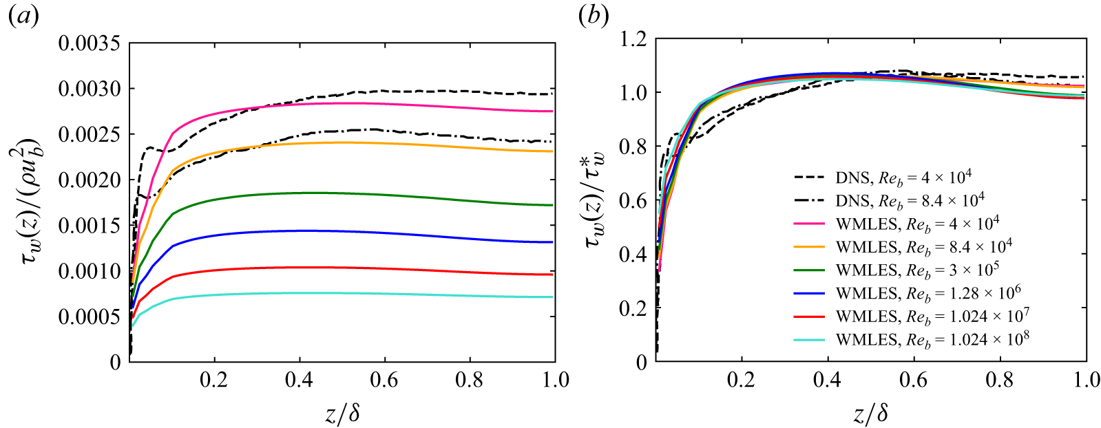
Distributions of the streamwise component of the local wall shear stress vector along the bottom wall (
 $y=0$
), computed from the wall model (2.5), are shown in figure 8. The profiles are normalised by either the bulk dynamic pressure (figure 8
a) or the mean wall shear stress (figure 8
b). The modelled transverse component of the shear stress is negligible in comparison, and is therefore omitted from the present analysis. In the first case, the wall shear stress decreases and levels off with increasing
 $\textit{Re}_b$
, indicating a clear tendency towards a uniform distribution around the duct perimeter at higher Reynolds numbers. This behaviour is consistent with the asymptotic arguments of Spalart et al. (Reference Smagorinsky2018), according to which wall friction should become uniform everywhere except in the immediate vicinity of the corners. Conversely, wall scaling yields nearly universal profiles at high Reynolds numbers, with an almost flat distribution away from the corners. The comparison with DNS profiles at
 $\textit{Re}_b=40\,000$
and
 $84\,000$
shows that WMLES reproduce the average wall shear stress, but fail to capture the sharp variations in the immediate vicinity of the corners. In the second case, the figure shows a clear tendency for the distributions to become universal and nearly flat sufficiently far from the side wall, as theoretically hypothesised by Spalart et al. (Reference Smagorinsky2018).
Distributions of local wall shear stress at the bottom wall: (a) bulk dynamic pressure normalisation; (b) mean wall shear stress normalisation.

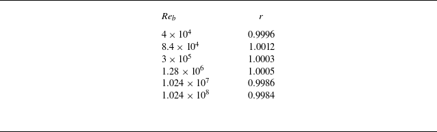
To assess the internal consistency of the WMLES, table 3 reports the ratio between the mean streamwise wall shear stress along the bottom wall of the square duct, as estimated from the wall model (2.5), and the perimeter-averaged wall shear stress
 $\tau _w^*$
, for increasing bulk Reynolds numbers. The resulting values remain very close to unity, ranging from 0.9984 to 1.0012. This confirms both the consistency of the wall-model formulation and the adequacy of the averaging intervals used to achieve statistical convergence.
Ratio
 $r=\langle \tau _w(z)|_{y=0}\rangle /\tau _w^*$
as a function of the bulk Reynolds number. Here,
 $\tau _w(z)|_{y=0}$
denotes the distribution of the streamwise component of the wall shear stress along the bottom wall of the square duct, as estimated from the wall model (2.5), and angle brackets denote spatial and temporal averaging.

Table 3. Long description
A table with two columns and seven rows. The first column is labeled Re_b and the second column is labeled r. The table presents the following data: Row 1: Re_b, 4 x 10^4; r, 0.9996. Row 2: Re_b, 8.4 x 10^4; r, 1.0012. Row 3: Re_b, 3 x 10^5; r, 1.0003. Row 4: Re_b, 1.28 x 10^6; r, 1.0005. Row 5: Re_b, 1.024 x 10^7; r, 0.9986. Row 6: Re_b, 1.024 x 10^8; r, 0.9984. The table assesses the internal consistency of the WMLES by reporting the ratio between the mean streamwise wall shear stress along the bottom wall of the square duct, as estimated from the wall model, and the perimeter-averaged wall shear stress for increasing bulk Reynolds numbers. The resulting values remain very close to unity, ranging from 0.9984 to 1.0012, confirming the consistency of the wall-model formulation and the adequacy of the averaging intervals used to achieve statistical convergence.
3.4. Friction factor
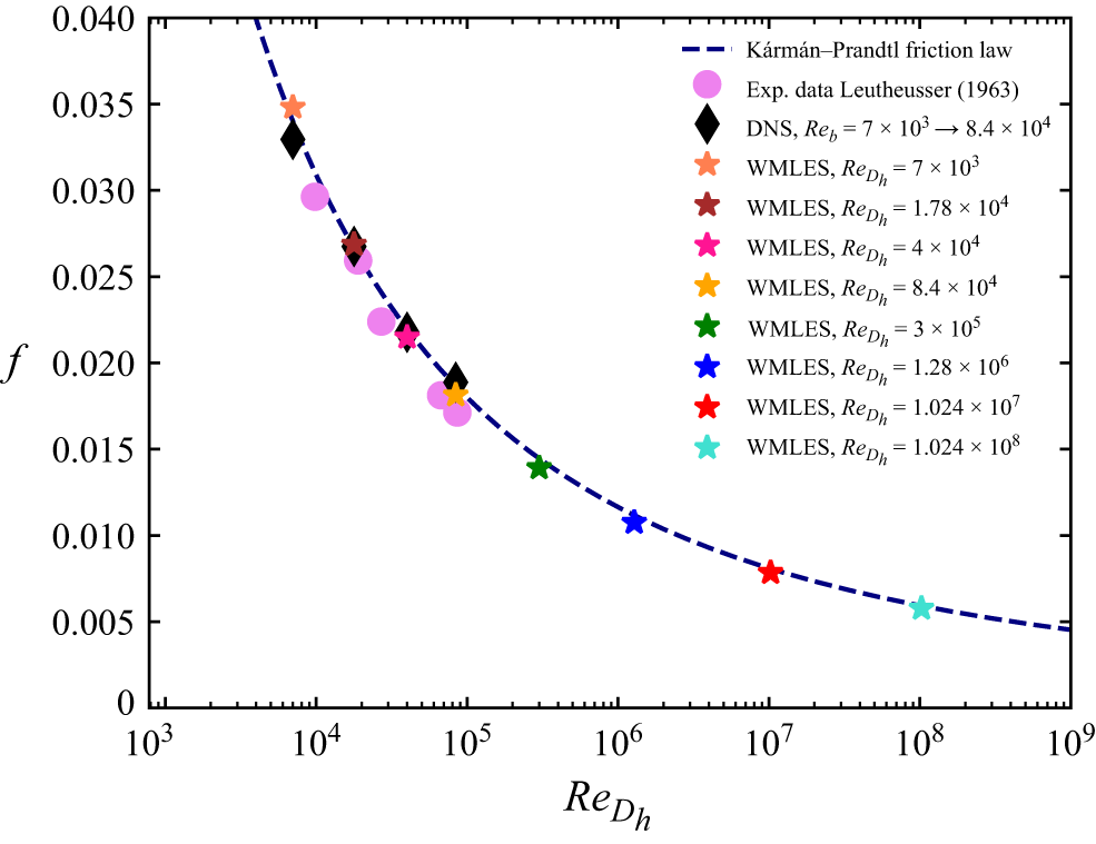
The analysis of the friction factor in duct flows is crucial for many engineering applications. It is commonly accepted (e.g. Schlichting & Gersten Reference Pullin, Inoue and Saito2016) that friction data for ducts of complex shape collapse onto the curves for canonical flows, provided that the bulk Reynolds number is defined with an appropriate length scale. The most widely used choice is the hydraulic diameter
 $D_h = 4A/P$
, where
 $A$
is the area, and
 $P$
is the perimeter of the duct cross-section. Pirozzoli et al. (Reference Pirozzoli2018) provided evidence that this collapse reflects the universality of the wall law, even for ducts of non-circular shape. In the present case of a square duct,
 $D_h = 2\delta$
, and the Reynolds number based on
 $D_h$
coincides with the bulk Reynolds number,
 $\textit{Re}_{D_h}=\textit{Re}_b$
. The computed friction factors
 $f=8\tau _w^*/(\rho u_b^2)$
are therefore reported as a function of
 $\textit{Re}_{D_h}=\textit{Re}_b$
in figure 9. Reference DNS data (Pirozzoli et al. Reference Pirozzoli2018; Modesti & Pirozzoli Reference Marin, Vinuesa, Obabko and Schlatter2022) and experimental measurements (Leutheusser Reference Launder and Ying1963) are also shown. For reference, figure 9 also reports the Kármán–Prandtl theoretical friction law for turbulent flow in a smooth circular pipe:
 \begin{equation} f^{-1/2} = 2\log _{10}\big (\textit{Re}_{D_h}f^{1/2}\big ) - 0.8 . \end{equation}
The WMLES data fall within the scatter of the experimental data, and exhibit excellent agreement with the DNS data at overlapping Reynolds numbers, with an error of approximately
 $4\,\%$
. This gives confidence in extrapolating the WMLES results beyond the envelope accessible to DNS and experiments. In fact, at very high Reynolds numbers, the WMLES results still agree with (3.4), falling just slightly below the theoretical relation. This finding supports continued validity of the Kármán–Prandtl friction law for ducts with complex cross-section also at Reynolds number not achievable in DNS and experiments.
Friction factor
 $f=8\tau _w^*/(\rho u_b^2)$
as a function of the Reynolds number based on the hydraulic diameter
 $\textit{Re}_{D_h}=u_bD_h/\nu =u_b2\delta /\nu =\textit{Re}_b$
. The dashed line denotes the reference Kármán–Prandtl friction curve (3.4). Symbols denote experimental data of Leutheusser (Reference Launder and Ying1963), DNS data of Pirozzoli et al. (Reference Pirozzoli2018) and Modesti & Pirozzoli (Reference Marin, Vinuesa, Obabko and Schlatter2022), and computed WMLES results.

3.5. Strength of the secondary motions
Secondary motions play a key role in redistributing momentum in ducts with non-circular cross-section. Although relatively weak, they are highly persistent, as quantified by Modesti et al. (Reference Modesti and Pirozzoli2018). Their asymptotic behaviour at high Reynolds number, however, remains unclear, particularly regarding whether their intensity scales with the bulk or the friction velocity. To address this issue, we examine the Reynolds number scaling of the kinetic energy associated with the mean cross-stream motion, integrated over the duct cross-section
 $A$
:
 \begin{equation} K_s = \frac {1}{2}\rho \int \big ({W}^2+{V}^2\big )\,{\mathrm{d}}A . \end{equation}
Figure 10 reports the square root of
 $K_s$
normalised by either the bulk velocity (figure 10
a) or the friction velocity (figure 10
b). The DNS data (black symbols) are inconclusive in this respect:
 $u_b$
scaling suggests a peak at
 $\textit{Re}_b \approx 40\,000$
followed by mild decline, while
 $u_\tau ^*$
scaling indicates continuing growth. The WMLES in the same moderate-
 $\textit{Re}$
range yield similar magnitudes, albeit with slightly different trends. Since the wall model is not expected to be fully accurate without a logarithmic layer, these differences in the low-Reynolds-number end are to be expected. The WMLES results at much higher Reynolds number yield important insight into the asymptotic behaviour. In fact, we see that the bulk-velocity scaling yields slow decay of
 $K_s$
, whereas the friction-velocity scaling yields an initial rise followed by a plateau for
 $\textit{Re}_b\gt 300\,000$
. The issue of the scaling of secondary motions has indeed always been controversial, and was also discussed by De Graaff & Eaton (Reference Gessner and Jones2000) for the boundary layer case. They suggested a mixed scaling based on
 $\sqrt {u_b\,u_\tau ^*}$
, which we have assessed in figure 10(c). The mixed velocity is found to be a valid scaling unit for low and moderate Reynolds numbers, compared to the friction velocity in figure 10(b), but it demonstrates a nearly monotonic decline at high Reynolds numbers, which is less pronounced than when using the bulk velocity in figure 10(a).
Square root of kinetic energy of the secondary motions integrated over the duct cross-section, scaled by (a) the bulk velocity
 $u_b$
, (b) the friction velocity
 $u_\tau ^*$
, and (c) the mixed velocity
 $\sqrt {u_b\,u_\tau ^*}$
. Here,
 $A=4 \delta ^2$
denotes the cross-sectional area. The black symbols denote DNS data of Pirozzoli et al. (Reference Pirozzoli2018) and Modesti & Pirozzoli (Reference Marin, Vinuesa, Obabko and Schlatter2022).

Figure 10. Long description
Three scatter plots depict the square root of kinetic energy of the secondary motions integrated over the duct cross-section, scaled by different velocities. Panel A: The scatter plot shows the square root of kinetic energy scaled by the bulk velocity. The x-axis represents the bulk Reynolds number (Reb) ranging from 10^4 to 10^9, and the y-axis represents the scaled kinetic energy ranging from 0 to 0.01. Various symbols denote different data sets, including DNS data and WMLES data with different Reynolds numbers. Panel B: The scatter plot shows the square root of kinetic energy scaled by the friction velocity. The x-axis represents the bulk Reynolds number (Reb) ranging from 10^4 to 10^9, and the y-axis represents the scaled kinetic energy ranging from 0 to 0.2. Various symbols denote different data sets, including DNS data and WMLES data with different Reynolds numbers. Panel C: The scatter plot shows the square root of kinetic energy scaled by the mixed velocity. The x-axis represents the bulk Reynolds number (Reb) ranging from 10^4 to 10^9, and the y-axis represents the scaled kinetic energy ranging from 0 to 0.04. Various symbols denote different data sets, including DNS data and WMLES data with different Reynolds numbers. The legend indicates the different data sets and their corresponding symbols.
Contours of (a–c) convective, (d–f) turbulence and (g–i) viscous contributions to the budget of mean streamwise momentum equation (3.6), for (a,d,g)
 $\textit{Re}_b=4 \times 10^4$
, (b,e,h)
 $\textit{Re}_b=1.28 \times 10^6$
and (c, f,i)
 $\textit{Re}_b=1.024 \times 10^8$
. The black contours in (a,d,g) correspond to the DNS data of Pirozzoli et al. (Reference Pirozzoli2018). The dashed line denotes the position of the exchange point along the duct perimeter. All terms have been normalised with outer units
 $(\rho u_b^2/\delta )$
.

Contours of (a–c) convective, (d–f) turbulence and (g–i) viscous contributions to the mean streamwise momentum budget (3.6), for (a,d,g)
 $\textit{Re}_b=4 \times 10^4$
, (b,e,h)
 $\textit{Re}_b=1.28 \times 10^6$
and (c, f,i)
 $\textit{Re}_b=1.024 \times 10^8$
. The black contours in (a,d,g) correspond to the DNS data of Pirozzoli et al. (Reference Pirozzoli2018). The dashed line denotes the position of the exchange point along the duct perimeter. All terms have been normalised with
 $({u_\tau ^*}^2/\delta )$
units.

Figure 12. Long description
Panel A: A heat map showing the convective contribution to the mean streamwise momentum budget at a Reynolds number of 4 x 10^4. The x-axis is labeled z/delta and ranges from 0 to 2. The y-axis is labeled y/delta and ranges from 0 to 2. The color scale ranges from -8 to 8, with red indicating lower values and blue indicating higher values. The black contours correspond to the DNS data of Pirozzoli et al. (2018). The dashed line denotes the position of the exchange point along the duct perimeter. Panel B: A heat map showing the convective contribution to the mean streamwise momentum budget at a Reynolds number of 1.28 x 10^6. The x-axis is labeled z/delta and ranges from 0 to 2. The y-axis is labeled y/delta and ranges from 0 to 2. The color scale ranges from -8 to 8, with red indicating lower values and blue indicating higher values. The dashed line denotes the position of the exchange point along the duct perimeter. Panel C: A heat map showing the convective contribution to the mean streamwise momentum budget at a Reynolds number of 1.024 x 10^8. The x-axis is labeled z/delta and ranges from 0 to 2. The y-axis is labeled y/delta and ranges from 0 to 2. The color scale ranges from -8 to 8, with red indicating lower values and blue indicating higher values. The dashed line denotes the position of the exchange point along the duct perimeter. Panel D: A heat map showing the turbulence contribution to the mean streamwise momentum budget at a Reynolds number of 4 x 10^4. The x-axis is labeled z/delta and ranges from 0 to 2. The y-axis is labeled y/delta and ranges from 0 to 2. The color scale ranges from -8 to 8, with red indicating lower values and blue indicating higher values. The black contours correspond to the DNS data of Pirozzoli et al. (2018). The dashed line denotes the position of the exchange point along the duct perimeter. Panel E: A heat map showing the turbulence contribution to the mean streamwise momentum budget at a Reynolds number of 1.28 x 10^6. The x-axis is labeled z/delta and ranges from 0 to 2. The y-axis is labeled y/delta and ranges from 0 to 2. The color scale ranges from -8 to 8, with red indicating lower values and blue indicating higher values. The dashed line denotes the position of the exchange point along the duct perimeter. Panel F: A heat map showing the turbulence contribution to the mean streamwise momentum budget at a Reynolds number of 1.024 x 10^8. The x-axis is labeled z/delta and ranges from 0 to 2. The y-axis is labeled y/delta and ranges from 0 to 2. The color scale ranges from -8 to 8, with red indicating lower values and blue indicating higher values. The dashed line denotes the position of the exchange point along the duct perimeter. Panel G: A heat map showing the viscous contribution to the mean streamwise momentum budget at a Reynolds number of 4 x 10^4. The x-axis is labeled z/delta and ranges from 0 to 2. The y-axis is labeled y/delta and ranges from 0 to 2. The color scale ranges from -8 to 8, with red indicating lower values and blue indicating higher values. The dashed line denotes the position of the exchange point along the duct perimeter. Panel H: A heat map showing the viscous contribution to the mean streamwise momentum budget at a Reynolds number of 1.28 x 10^6. The x-axis is labeled z/delta and ranges from 0 to 2. The y-axis is labeled y/delta and ranges from 0 to 2. The color scale ranges from -0.3 to 0.3, with red indicating lower values and blue indicating higher values. The dashed line denotes the position of the exchange point along the duct perimeter. Panel I: A heat map showing the viscous contribution to the mean streamwise momentum budget at a Reynolds number of 1.024 x 10^8. The x-axis is labeled z/delta and ranges from 0 to 2. The y-axis is labeled y/delta and ranges from 0 to 2. The color scale ranges from -0.005 to 0.005, with red indicating lower values and blue indicating higher values. The dashed line denotes the position of the exchange point along the duct perimeter.
Contours of (a–c) convective, (d–f) turbulence and (g–i) viscous contributions to the
 $y$
-momentum budget (3.7), for (a,d,g)
 $\textit{Re}_b=4 \times 10^4$
, (b,e,h)
 $\textit{Re}_b=1.28 \times 10^6$
and (c, f,i)
 $\textit{Re}_b=1.024 \times 10^8$
. The black contours in (a,d,g) correspond to the DNS data of Pirozzoli et al. (Reference Pirozzoli2018). The dashed line denotes the position of the exchange point along the duct perimeter. All terms have been normalised with
 $({u_\tau ^*}^2/\delta )$
units.

Further insight can be obtained by considering the mean streamwise momentum budget equation, which reads (Modesti et al. Reference Modesti and Pirozzoli2018)
 \begin{align} \underbrace {{V}\frac {\partial {U}}{\partial y}+{W}\frac {\partial {U}}{\partial z}}_{\textrm{convective term}}+\underbrace {\left (\frac {\partial \langle \overline {u}\,\overline {v} \rangle }{\partial y}+\frac {\partial \langle \overline {u}\,\overline {w} \rangle }{\partial z}+\frac {\partial \tau _{12}}{\partial y}+\frac {\partial \tau _{13}}{\partial z}\right )}_{\textrm{turbulence term}}-\underbrace {\nu \left (\frac {\partial ^2{U}}{\partial y^2}+\frac {\partial ^2{U}}{\partial z^2}\right )}_{\textrm{viscous term}}+\,\langle \varPi \rangle =0, \end{align}
in which the first term includes the effect of convection from the secondary flows, the second term the Reynolds stress gradients, the third term the viscous diffusion, and the last term is the time average of the driving body force. Here,
 $\langle \overline {u}\,\overline {v} \rangle$
and
 $\langle \overline {u}\,\overline {w} \rangle$
denote the resolved parts of the turbulent shear stresses, whereas
 $\tau _{12}$
and
 $\tau _{13}$
are the streamwise and time averages of the subgrid-scale shear stresses, as defined in (2.3). The distributions of the budget terms over the duct cross-section are presented in figures 11 and 12, scaled by the ratio of either the square bulk velocity or friction velocity, and the side length, respectively. All terms in the budget exhibit large variations within approximately 50 wall units from the walls (Pirozzoli et al. Reference Pirozzoli2018). Hence the colour scale is properly selected to resolve small variations taking place in the bulk flow. In all cases, we find that the viscous contribution away from walls is negligible, and the leading-order balance is between turbulence and mean convection. Convective transport plays a key role in correspondence of corners and wall bisectors, along which momentum redistribution occurs, and close balance with the turbulent term is observed. Figure 11 further shows that outer scaling yields decreasing intensity of each budget term with the Reynolds number, corroborating trends seen in figures 2 and 4. On the other hand, when the friction velocity is used for normalisation (figure 12), the magnitude of the convective and turbulence terms is barely affected by variations in Reynolds number.
The mean momentum balance in the two transverse directions can be analysed in a similar manner. The balance equation in the
 $y$
direction reads
 \begin{equation} \underbrace {{V}\frac {\partial {V}}{\partial y} +{W}\frac {\partial {V}}{\partial z}}_{\textrm{convective term}} +\frac {1}{\rho }\frac {\partial \langle \overline {p} \rangle }{\partial y} +\underbrace {\left (\frac {\partial \langle \overline {v}\,\overline {v} \rangle }{\partial y} +\frac {\partial \langle \overline {v}\,\overline {w} \rangle }{\partial z}\right )}_{\textrm{turbulence term}} -\underbrace {\nu \left (\frac {\partial ^2{V}}{\partial y^2} +\frac {\partial ^2{V}}{\partial z^2}\right )}_{\textrm{viscous term}} =0, \end{equation}
where
 $\langle \overline {p} \rangle$
denotes the mean filtered pressure, and
 $\langle \overline {v}\,\overline {w} \rangle$
is the resolved cross-plane turbulent shear stress. Since the isotropic part of the subgrid stresses is absorbed into the modified pressure (see § 2), only resolved stress components appear explicitly in the above balance, and the pressure gradient is not evaluated separately. Contours of the individual terms in (3.7) over the duct cross-section are shown in figure 13. As in previous figures, the friction velocity and the side length are again used for normalisation, and the colour scale is selected to resolve the small variations in the bulk region. For all cases, the dominant contribution is the resolved turbulent term, whose magnitude is largest near the walls, and decreases towards the duct core. The resolved convective and viscous terms, by contrast, are primarily confined to the near-wall region and the duct corners. The figure further indicates that the magnitudes of the turbulent and convective contributions vary only weakly with Reynolds number.
These results support the view of Spalart et al. (Reference Smagorinsky2018) that secondary motions scale with the friction velocity, a result of considerable theoretical significance. A possible physical interpretation for the
 $u_\tau ^*$
scaling is suggested by the work of Brundrett & Baines (Reference Brundrett and Baines1964), who analysed the origin and dissipation of secondary motions in terms of the streamwise vorticity equation. Based on experimental observations, they showed that vorticity is produced away from the corners and subsequently transported towards the corner regions by convection, where it is balanced by viscous diffusion. When scaled by the global friction velocity, production and convection terms are nearly Reynolds number independent. To maintain vorticity balance, the near-wall diffusion term must also exhibit weak Reynolds number dependence. This behaviour can be understood in terms of the progressive penetration of secondary motions into the duct corners as the Reynolds number increases. This enhances spatial gradients in the secondary-velocity field, increasing the higher-order derivatives and vorticity gradients that govern diffusion. In this way, all terms remain commensurate when expressed in inner units. Brundrett & Baines (Reference Brundrett and Baines1964) further noted, in agreement with the experimental findings of Leutheusser (Reference Launder and Ying1963), that the approach of secondary motions towards the walls is analogous to the progressive thinning of the viscous sublayer with increasing Reynolds number, a well-established feature of canonical wall-bounded flows. Within this framework, the observed scaling of secondary motions with the global friction velocity can be interpreted as a natural consequence of the underlying vorticity balance.
These findings indicate that secondary currents remain of the same order as other turbulent fluctuations in the infinite-Reynolds-number limit: they retain a distorting influence but do not dominate. Conversely, the decay of
 $K_s$
with
 $u_b$
scaling implies that secondary motions are primarily a finite-Reynolds-number phenomenon. Viewed in outer units, the asymptotic state of square-duct turbulence corresponds to plug flow with finite slip at the wall, as suggested by figures 1 and 5(b). In this regime, turbulence fluctuations and secondary motions become asymptotically negligible in outer units, and flow distortions are confined to an increasingly thin near-wall region and the duct corners. This conclusion parallels the Couette flow results of Cheng et al. (Reference Cheng, Pullin and Samtaney2022), the theoretical arguments of Pullin et al. (Reference Prandtl2013), and the experimental observations of Gessner & Jones (Reference Gavrilakis1965) and Launder & Ying (Reference Larsson, Kawai, Bodart and Bermejo-Moreno1972).
4. Conclusions
Turbulent flow in a square duct has been investigated over a wide range of bulk Reynolds numbers using wall-modelled large-eddy simulations (WMLES). The classical Smagorinsky model with van Driest near-wall damping was employed to model the subgrid-scale stresses, and an equilibrium wall model based on the logarithmic law was used to represent the near-wall region. Simulations were performed on a uniform Cartesian mesh, enabling exploration of Reynolds numbers far beyond the reach of DNS (and experiments as well), with modest computational resources. The simulations reproduced the secondary flows and the bulging of streamwise-velocity contours towards the corners, consistent with experiments and DNS. Quantitative agreement with DNS was achieved at overlapping Reynolds numbers, particularly for mean velocity contours, turbulence statistics along the wall bisector, and wall shear stress distributions. The WMLES predictions were also consistent with the Prandtl friction law based on the hydraulic diameter, even in the high-Reynolds-number limit. Hence a primary conclusion that we can draw from our numerical study is that WMLES are capable of providing accurate prediction for turbulent flow in ducts with relatively complex cross-section, and they are especially suitable to provide accurate information about the behaviour of the secondary motions that arise in this type of flow. Reduced accuracy is found in the proximity of corners, which is most evident in the local wall shear stress profiles. This shortcoming likely reflects the limitations of the equilibrium logarithmic wall model in geometrically complex regions.
Analysis of the kinetic energy of the secondary motions has further revealed that although these motions persist at all Reynolds numbers, their bulk-velocity-scaled intensity decays monotonically, while friction-velocity scaling leads to a plateau at large
 $\textit{Re}_b$
. Similar conclusions hold true for the various terms in the mean momentum budget equations. This suggests that secondary motions are essentially a finite-Reynolds-number effect, and that the asymptotic state of square-duct turbulence corresponds to a plug-like velocity profile. These findings parallel conclusions previously drawn for plane Poiseuille and Couette flows.
The application of the WMLES methodology naturally raises the question of whether the classical turbulence assumptions embedded in both the subgrid-scale closure and the wall-stress model affect the results, in particular the recovered scaling of the intensity of the secondary motions with the friction velocity. Indeed, WMLES cannot be used to discover or falsify the logarithmic law of the wall, nor to establish near-wall scaling laws independently of classical theory. Classical arguments underlie both the subgrid modelling away from the wall and the wall-stress closure in the near-wall region. Secondary motions, however, are not directly prescribed by either component of the modelling. The wall model enforces only the local relation between wall-parallel velocity and wall shear stress, while the subgrid model provides an eddy viscosity without imposing cross-plane Reynolds stress anisotropy. Furthermore, the transverse mean momentum equations governing secondary motions involve gradients of the resolved Reynolds stresses, which are not fixed a priori by the modelling assumptions. The structure, intensity and scaling of secondary motions therefore emerge from the resolved dynamics, and are not constrained in advance to scale with either the bulk or the friction velocity. If the present analysis were purely circular, then one would expect the secondary motions to scale trivially with the imposed near-wall velocity scale at all Reynolds numbers. Instead, both DNS and WMLES data exhibit a non-monotonic transition: at moderate Reynolds numbers, the scaling is ambiguous, and even differs between DNS and WMLES, whereas a clear asymptotic trend appears only at sufficiently large Reynolds numbers. Such behaviour is not prescribed by the modelling framework, and would not arise in a strictly circular construction.
Further evidence that the modelling assumptions do not uniquely determine the outcome is provided by Cheng & Samtaney (Reference Cheng and Samtaney2014), who examined the debate on the appropriate scaling law for the overlap region of wall-bounded turbulent flows. They performed WMLES using both power-law and logarithmic wall models, and found that the resulting statistics preferentially followed logarithmic scaling in both cases. This suggests that the resolved flow is not dictated solely by the particular functional form imposed in the wall model, and that large-scale statistics may exhibit some robustness to the wall-stress closure. The trend was found to become clearer at higher Reynolds numbers, supporting the use of the logarithmic wall model in the present study. At the same time, Cheng & Samtaney (Reference Cheng and Samtaney2014) emphasised that their results were suggestive rather than conclusive, and that WMLES remain subject to modelling limitations.
One may further note that any numerical approach necessarily embeds, to some extent, classical turbulence assumptions through grid design, including DNS, which remains the most fundamental tool for establishing Reynolds number trends. However, DNS at the extreme Reynolds numbers considered here is currently infeasible, and the objective of the present study is not to replace DNS as a definitive arbiter of turbulence theory. Rather, our aim is to examine the logical consequences of classical asymptotic arguments in a flow configuration where secondary motions play a central dynamical role. In this sense, the present work should be regarded as a consistency test of classical theory in square-duct turbulence, rather than as an independent derivation of that theory. Similar methodological limitations, to varying degrees, apply to any finite-Reynolds-number numerical or experimental investigation. Within these constraints, we believe that WMLES can still provide meaningful insight into the asymptotic behaviour of secondary motions, provided that their assumptions and limitations are clearly recognised.
Future work will focus on the use of improved wall-stress closures, which could possibly improve the near-corner behaviour of WMLES, and on the extension to the study of heat transfer problems. Extension to other duct geometries, particularly rectangular ducts with varying aspect ratios, will be considered in future work in order to assess the generality of the scaling trends identified for the square duct.
Acknowledgements
We acknowledge that the results reported in this paper have been achieved using the EuroHPC Research Infrastructure resource LEONARDO based at CINECA, Casalecchio di Reno, Italy.
Funding
This research received no specific grant from any funding agency, commercial or not-for-profit sectors.
Declaration of interests
The authors report no conflict of interest.
Data availability statement
The data that support the findings of this study are openly available at the web page http://newton.dma.uniroma1.it/database/.


 Reb=2ubδ/ν
 Lx
 δ
 Nx
 Ny
 Nz
 Reτ=uτ∗δ/ν
 f=8τw∗/(ρub2)
 Δx∗,Δy∗,Δz∗
 Δtav∗uτ∗/δ
 δ/uτ∗

 U/ub

 W/ub
 0≤y/δ≤1
 z/δ=0.5
 Reb=2ubδ/ν
 ΠDNS
 ΠWMLES
 0≤y/δ≤1
 z/δ=0.5

 u∗=log(y∗)/0.41+5.2
 UCL∗
 ub∗
 UCL/ub

 r=⟨τw(z)|y=0⟩/τw∗
 τw(z)|y=0
 f=8τw∗/(ρub2)
 ReDh=ubDh/ν=ub2δ/ν=Reb

 ub
 uτ∗
 ubuτ∗
 A=4δ2

 Reb=4×10⁴
 Reb=1.28×10⁶
 Reb=1.024×10⁸
 (ρub2/δ)

 Reb=4×10⁴
 Reb=1.28×10⁶
 Reb=1.024×10⁸
 (uτ∗2/δ)

 y
 Reb=4×10⁴
 Reb=1.28×10⁶
 Reb=1.024×10⁸
 (uτ∗2/δ)

 Open access

