1 Introduction
Two-dimensional (2-D) inviscid, incompressible (ideal) fluid systems are governed by the Euler equations
 $$\begin{eqnarray}\displaystyle [\unicode[STIX]{x2202}_{t}-(\unicode[STIX]{x1D735}\unicode[STIX]{x1D713}\times \hat{\boldsymbol{z}})\boldsymbol{\cdot }\unicode[STIX]{x1D735}]~\unicode[STIX]{x1D714}=0;\quad \unicode[STIX]{x1D6FB}^{2}\unicode[STIX]{x1D713}=\unicode[STIX]{x1D714}, & & \displaystyle\end{eqnarray}$$
where
 $\unicode[STIX]{x1D713}$
is the fluid streamfunction in two dimensions, with fluid velocity
 $\boldsymbol{v}=-\unicode[STIX]{x1D735}\unicode[STIX]{x1D713}\times \hat{\boldsymbol{z}}$
and vorticity
 $\unicode[STIX]{x1D714}\hat{\boldsymbol{z}}=\unicode[STIX]{x1D735}\times \boldsymbol{v}$
. Flows described by (1.1) are often characterized by the emergence and persistence of coherent rotational flow structures known generally as vortices. When isolated, these structures are known to be long lived and stable (McWilliams Reference McWilliams1984). However, when subjected to externally imposed strain flows, such as those due to another nearby vortex or a boundary, vortex deformation and/or destruction can occur (Mariotti, Legras & Dritschel Reference Mariotti, Legras and Dritschel1994; Trieling, Beckers & Heijst Reference Trieling, Beckers and Van Heijst1997). Understanding the competition between strain and vorticity is an important goal of nonlinear fluid dynamics that is relevant to a variety of quasi-2-D fluid systems.
A particularly fruitful approach for investigating 2-D ideal fluids in the laboratory involves study of the dynamics of a magnetized pure electron plasma confined in a cylindrical Penning–Malmberg (PM) trap (O’Neil Reference O’Neil1999). In a PM trap, electrons perform axial bounce motion in an electrostatic potential well, while moving in the plane perpendicular to the magnetic field via guiding-centre
 $\boldsymbol{E}\times \boldsymbol{B}$
drift dynamics, where
 $\boldsymbol{E}$
and
 $\boldsymbol{B}$
are the electric and magnetic fields (Chen Reference Chen1984). When the magnetic field is strong and the bounce motion is rapid, the electrons behave approximately as rigid line charges. In this case, the 2-D dynamics of the electron density is described by the drift–Poisson equations
 $$\begin{eqnarray}\displaystyle \left[\unicode[STIX]{x2202}_{t}-\frac{1}{B}(\unicode[STIX]{x1D735}\unicode[STIX]{x1D719}\times \hat{\boldsymbol{z}})\cdot \unicode[STIX]{x1D735}\right]n=0;\quad \unicode[STIX]{x1D6FB}^{2}\unicode[STIX]{x1D719}=\frac{en}{\unicode[STIX]{x1D700}_{0}}, & & \displaystyle\end{eqnarray}$$
(SI units) where
 $\unicode[STIX]{x1D700}_{0}$
is the permittivity of free space,
 $n(x,y)$
is the electron density in two dimensions,
 $\unicode[STIX]{x1D719}(x,y)$
is the electric potential,
 $e$
is the electron charge, and the
 $\boldsymbol{E}\times \boldsymbol{B}$
drift velocity is
 $\boldsymbol{v}=-\unicode[STIX]{x1D735}\unicode[STIX]{x1D719}\times \hat{\boldsymbol{z}}/B$
. Equations (1.2) are isomorphic to the 2-D Euler equations (1.1) for ideal fluid flow, under the transformations
 $\unicode[STIX]{x1D714}\rightarrow en/B\unicode[STIX]{x1D700}_{0}$
and
 $\unicode[STIX]{x1D713}\rightarrow \unicode[STIX]{x1D719}/B$
(Driscoll & Fine Reference Driscoll and Fine1990). Thus, the electron density is analogous to the fluid vorticity, and the electric potential is analogous to the fluid streamfunction. This plasma/fluid correspondence has been used widely as a proxy to study the dynamics of 2-D ideal fluids (O’Neil Reference O’Neil1999).
Advantages of the electron plasma system for 2-D ideal fluid experiments include weak dissipation and free-slip boundary conditions, precise control over the initial vorticity distribution and external flows and the ability to image directly the vorticity field using a phosphor screen and a camera. Additionally, system parameters can be varied rapidly in electron plasma experiments, permitting studies across a wide range of conditions.
In the present work, we study the behaviour of a 2-D ideal vortex embedded in an external irrotational strain flow using laboratory experiments with electron plasma and vortex-in-cell simulations (Leonard Reference Leonard1980). The experiments utilize a PM electron plasma trap called the 8-segment trap (8ST) which was designed specifically to study 2-D vortex dynamics under the influence of external flows. It features a long electrode spanning the length of the plasma which is azimuthally segmented into eight pieces. It provides the capability to impose asymmetric boundary conditions without introducing 3-D effects. Additionally, initial axisymmetric vorticity profiles ranging from Gaussian to quasi-flat can be obtained. The experiments and simulations are compared with predictions of a theory assuming the vorticity is constant within an elliptical region (the elliptical patch model (Moore & Saffman Reference Moore, Saffman, Rogers, Olsen and Goldburg1971; Kida Reference Kida1981)). Specifically, we observe periodic orbits, equilibria and unstable modes corresponding to vortex destruction. For quasi-flat profiles, the results are in good quantitative agreement with the elliptical patch model (i.e. with no fitted parameters). However, smooth profiles are subject to inviscid damping of the dynamical orbits and modified stability properties. A preliminary report of these studies can be found in Hurst et al. (Reference Hurst, Danielson, Dubin and Surko2016).
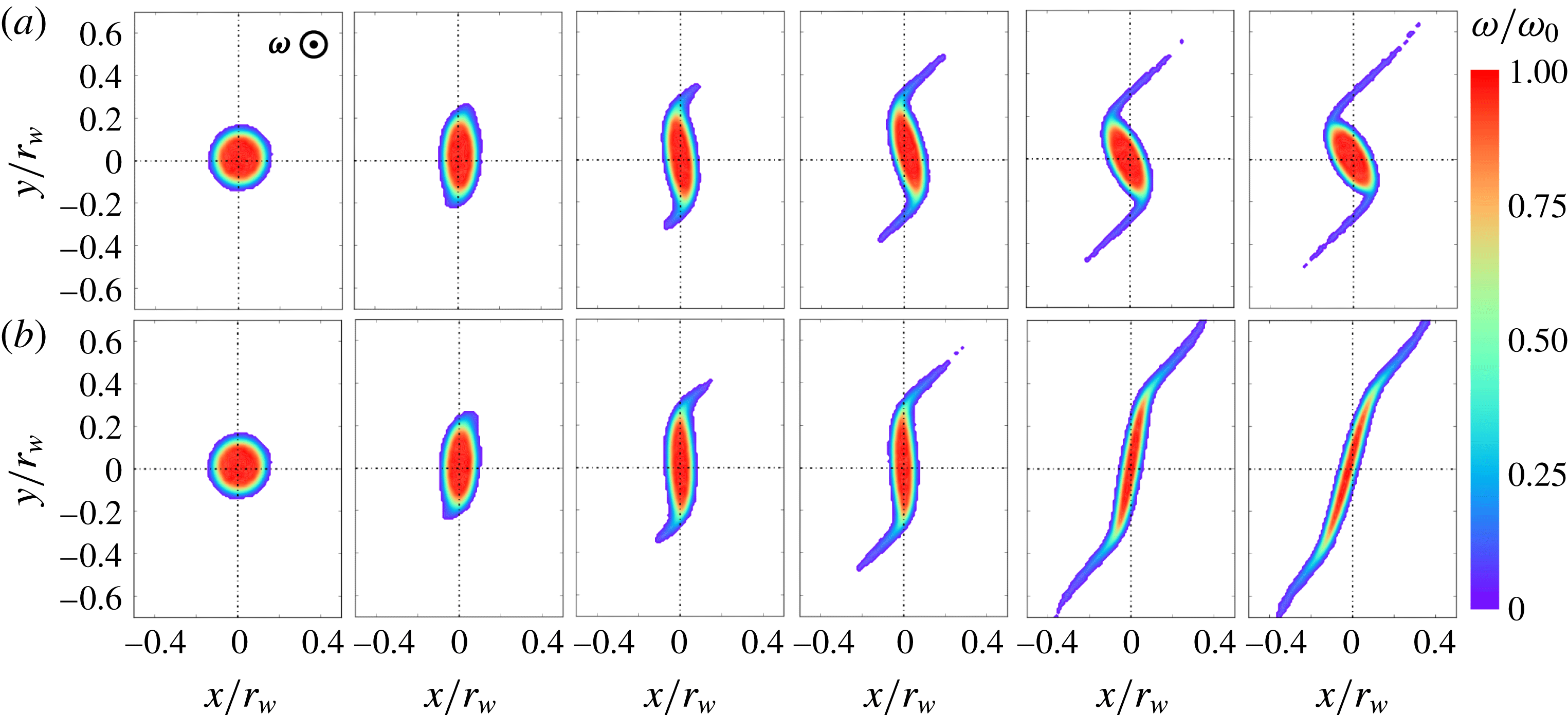
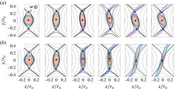
An example of experimental data obtained using the 8ST is shown in figure 1. Here, an initially axisymmetric vortex with a quasi-flat profile (shown in figure 5 b) is subjected to an externally imposed irrotational simple strain flow given by
 $$\begin{eqnarray}\displaystyle \unicode[STIX]{x1D713}_{s}={\textstyle \frac{1}{2}}\unicode[STIX]{x1D716}(x^{2}-y^{2});\quad \boldsymbol{v}_{\boldsymbol{ s}}=\unicode[STIX]{x1D716}(y\hat{\boldsymbol{x}}+x\hat{\boldsymbol{y}}), & & \displaystyle\end{eqnarray}$$
where
 $\unicode[STIX]{x1D716}$
is the strain rate, by electrically manipulating the boundary conditions in a way that preserves the 2-D dynamics. The strain is raised abruptly from zero to some value
 $\unicode[STIX]{x1D716}$
, and then held constant. Figure 1(a) shows the measured evolution of the vorticity distribution at
 $20~\unicode[STIX]{x03BC}\text{s}$
(
 $4.56\unicode[STIX]{x1D714}_{0}^{-1}$
) increments, where the ratio of applied strain magnitude to peak vorticity is
 $\unicode[STIX]{x1D716}/\unicode[STIX]{x1D714}_{0}\equiv \unicode[STIX]{x1D716}^{\ast }=0.116$
, with
 $\unicode[STIX]{x1D714}_{0}=228~\text{krad}~\text{s}^{-1}$
. The strain extracts filaments of vorticity from the periphery of the distribution, however the vortex core remains intact and elliptical, and continues to rotate in the counter-clockwise direction. Figure 1(b) shows the vorticity evolution for
 $\unicode[STIX]{x1D716}^{\ast }=0.130$
, with the same initial condition and time intervals as figure 1(a). In this case, elliptical distortion of the vortex core increases without bound, the orientation approaches the strain axis and the vortex is effectively destroyed.
Experimental data for the evolution of vorticity (electron density) under constant strain-to-vorticity ratio
 $\unicode[STIX]{x1D716}^{\ast }=$
(a) 0.116, (b) 0.130, for
 $t=0{-}22.8\unicode[STIX]{x1D714}_{0}^{-1}$
(at equal increments), and peak vorticity
 $\unicode[STIX]{x1D714}_{0}=228~\text{krad}~\text{s}^{-1}$
out of the page. Data are suppressed for
 $\unicode[STIX]{x1D714}<0.05\unicode[STIX]{x1D714}_{0}$
in order to remove noise. Spatial coordinates are scaled to the wall radius
 $r_{w}$
of the 8ST.

Vortex deformation in response to strain has received much attention in the literature, using a variety of different approaches. Theoretical progress has been facilitated by the elliptical patch model. In particular, exact solutions to the Euler equations (1.1) were found by Moore & Saffman (Reference Moore, Saffman, Rogers, Olsen and Goldburg1971) and Kida (Reference Kida1981) (henceforth MS71 and K81) for the equilibria and dynamics of an elliptical vortex patch in external shear and strain flows. Detailed studies of the stability of the these solutions have been conducted by Dritschel (Reference Dritschel1990). In contrast, theoretical study of a smooth vorticity distribution in an external strain flow is a more daunting task, and progress has been made so far only in cases where the nonlinearity can be handled perturbatively, for example, in the limit of weak or strong strain (Hunt & Carruthers Reference Hunt and Carruthers1990; Lingevitch & Bernoff Reference Lingevitch and Bernoff1995; Balmforth, Smith & Young Reference Balmforth, Smith and Young2001), or short time scales (Weiss Reference Weiss1991; Schecter et al. Reference Schecter, Dubin, Cass, Driscoll, Lansky and O’Neil2000; Turner, Gilbert & Bassom Reference Turner, Gilbert and Bassom2008).
Experimental studies of strained vortices have focused primarily on laboratory water tanks (Trieling et al. Reference Trieling, Beckers and Van Heijst1997), demonstrating vortex deformation, destruction and partial destruction, or ‘vortex stripping’, where thin filaments of vorticity are extracted from the edge of the vortex by the applied strain. However, viscous effects in these experiments have prevented a direct comparison with the elliptical patch theory. Numerical experiments have been conducted using the contour dynamics technique, where nested contours of piecewise-constant vorticity are advected dynamically (Zabusky Reference Zabusky1979; Dritschel Reference Dritschel1989). This procedure has qualitatively reproduced the vortex stripping and destruction phenomena observed in the laboratory, and it has also provided other useful insights (Mariotti et al. Reference Mariotti, Legras and Dritschel1994; Legras, Dritschel & Caillol Reference Legras, Dritschel and Caillol2001; Mitchell & Rossi Reference Mitchell and Rossi2008).
Notable previous results using electron plasma fluids include laboratory studies of vortex crystal formation (Fine et al.
Reference Fine, Cass, Flynn and Driscoll1995) and stability (Durkin & Fajans Reference Durkin and Fajans2000), inviscid damping of vortex distortions (Schecter et al.
Reference Schecter, Dubin, Cass, Driscoll, Lansky and O’Neil2000), vortex merger events (Mitchell & Driscoll Reference Mitchell and Driscoll1996; Soga et al.
Reference Soga, Kiwamoto, Sanpei and Aoki2003) and studies of 2-D turbulent cascades (Kawai et al.
Reference Kawai, Kiwamoto, Soga and Aoki2007; Chen, Maero & Rome Reference Chen, Maero and Rome2017). Most of these experiments focused on the free relaxation of an initial vorticity distribution with azimuthally symmetric boundary conditions. Some work has also been done with asymmetric boundary conditions (Chu et al.
Reference Chu, Wurtele, Notte, Peurrung and Fajans1993; Schecter et al.
Reference Schecter, Dubin, Cass, Driscoll, Lansky and O’Neil2000), although these experiments may have been subject to 3-D effects which violate the plasma/fluid analogy. Particularly relevant is the work of Eggleston (Reference Eggleston1994), in which electron vortices are subjected to irrotational
 $\boldsymbol{E}\times \boldsymbol{B}$
shear due to an externally imposed radial electric field.
Approximate 2-D vortices are commonly observed in geophysical fluids, strongly magnetized plasmas, astrophysical disks and a variety of other flows in engineering and industrial settings. Vortices form regularly in the oceans and atmospheres of Earth and other planets, and are important for heat and chemical transport (Dritschel & Legras Reference Dritschel and Legras1993). It is well known that a strong magnetic field in a plasma causes a spatial asymmetry which can result in quasi-2-D drift dynamics perpendicular to the field (Hasegawa & Mima Reference Hasegawa and Mima1978; Montgomery & Turner Reference Montgomery and Turner1980; Terry Reference Terry2000). This phenomenology is applicable to a wide range of laboratory and astrophysical plasmas, including magnetically confined plasmas for controlled nuclear fusion. A quasi-2-D polar geometry is commonly found in astrophysical disks such as galaxies and accretion disks. It is thought that vortices may form in these disks, which could impact planet formation (Godon & Livio Reference Godon and Livio1999) and momentum transport (Lithwick Reference Lithwick2009). Interestingly, recent theoretical work suggests the existence of a 2-D fluid-like flow of space–time near the event horizon of large black holes (Adams, Chesler & Liu Reference Adams, Chesler and Liu2014). The stability and behaviour of 2-D vortices is of importance in various engineering flows including, for example, airfoil wakes (Moore & Saffman Reference Moore, Saffman, Rogers, Olsen and Goldburg1971) and mixing processes (Voth, Haller & Gollub Reference Voth, Haller and Gollub2002). Finally, the filamentation behaviour described here is ubiquitous in vortex dynamics; it is closely related to the forward enstrophy cascade familiar to 2-D turbulence theory (Tabeling Reference Tabeling2002). A key theme in many of these systems is that the fluid dynamics and transport properties can be significantly affected by the presence of vortices, and so their stability under external flow is of broad interest.
The remainder of the paper is organized as follows. In § 2, we discuss further details of the plasma/fluid analogy and the experimental and numerical procedures. In § 3, we present a review of relevant theoretical work. In § 4, we present experimental and numerical data, and compare the results to theoretical predictions. Finally, in § 5 we conclude with a discussion of the results and prospects for future work.
2 Experimental procedure
This section contains a discussion of how 2-D ideal fluid vortices can be studied in the presence of external strain using magnetized electron plasmas. A description of the analogy between these plasmas and fluid vortices is given, and details of the experimental procedure are discussed. Finally, numerical methods are discussed in which a vortex-in-cell algorithm (Leonard Reference Leonard1980) is implemented to support and extend the experimental results. Further information about the experimental technique can be found in Hurst, Danielson & Surko (Reference Hurst, Danielson and Surko2018).
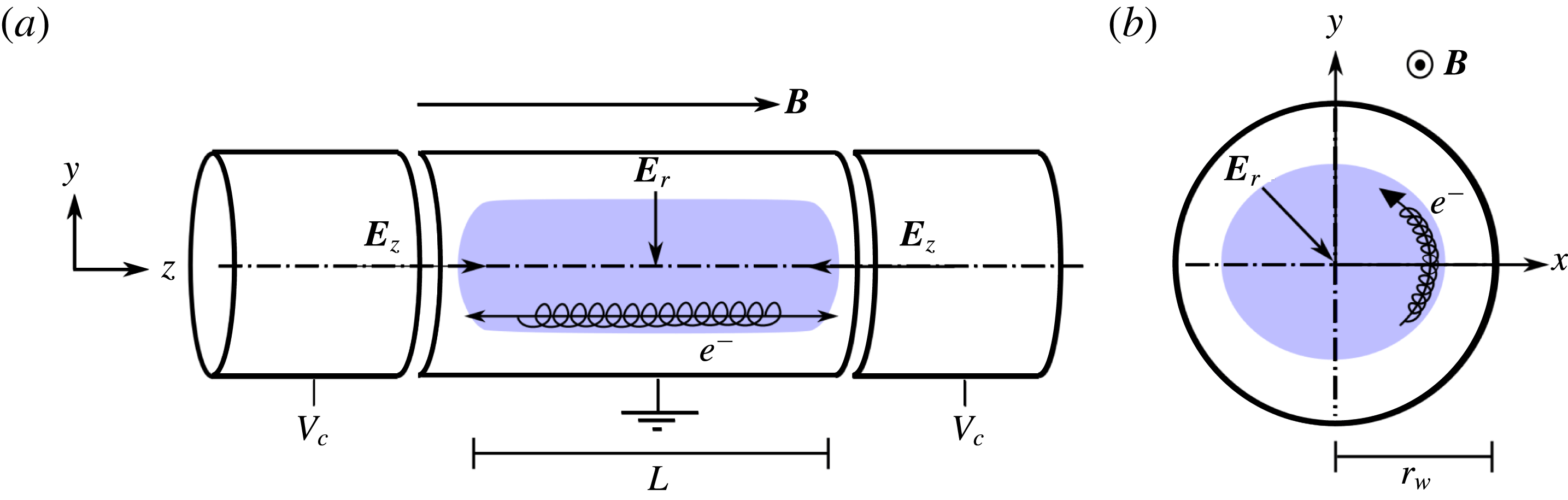
Sketch of electron motion in a PM trap. (a)
 $(y,z)$
and (b)
 $(x,y)$
views are shown, with axial confinement voltages
 $V_{c}$
, axial and radial electric fields
 $\boldsymbol{E}_{\boldsymbol{z}}$
and
 $\boldsymbol{E}_{\boldsymbol{r}}$
and magnetic field
 $\boldsymbol{B}$
. Electron trajectories are depicted, including (a) the axial bounce motion and (b) the perpendicular
 $\boldsymbol{E}\times \boldsymbol{B}$
drift motion, as well as the small-scale gyromotion in both panels.

2.1 The analogy between electron plasmas and fluid vortices
Non-neutral plasmas consisting only of electrons are routinely confined in a cylindrical geometry using a strong, constant axial magnetic field
 $\boldsymbol{B}=B\hat{\boldsymbol{z}}$
for radial confinement and electrostatic potentials
 $\unicode[STIX]{x1D719}(z)$
for axial confinement. This configuration is known as a Penning–Malmberg (PM) trap (Dubin & O’Neil Reference Dubin and O’Neil1999); a schematic diagram of this type of apparatus is shown in figure 2. Confinement in a PM trap is sufficiently good that the plasma can reach a steady-state thermal equilibrium characterized by a temperature
 $T$
. In the presence of a strong magnetic field, the electrons perform small, high-frequency gyro-orbits perpendicular to the magnetic field with radius
 $r_{g}=mv_{T}/eB$
and frequency
 $f_{g}=eB/2\unicode[STIX]{x03C0}m$
, where
 $v_{T}=(T/m)^{1/2}$
is the thermal velocity, and
 $e$
and
 $m$
are the electron charge and mass. Furthermore, when electric fields are present, the gyrating electrons drift perpendicular to
 $\boldsymbol{B}$
with velocity
 $\boldsymbol{v}=B^{-2}\,\boldsymbol{E}\times \boldsymbol{B}$
(Chen Reference Chen1984). Electric fields are generated by the non-neutral plasma itself and by the boundary conditions via the Poisson equation,
 $\unicode[STIX]{x1D6FB}^{2}\unicode[STIX]{x1D719}=en/\unicode[STIX]{x1D700}_{0}$
. Often, the plasma density is axisymmetric and quasi-uniform within radius
 $r_{v}$
, so the self-electric field is radial, and the drift motion is azimuthal and periodic about the plasma centroid with frequency
 $f_{v}=en/4\unicode[STIX]{x03C0}B\unicode[STIX]{x1D700}_{0}$
(Danielson et al.
Reference Danielson, Dubin, Greaves and Surko2015). Parallel to the magnetic field, electrons bounce rapidly between the endcap confinement potentials at frequency
 $f_{b}=v_{T}/2L$
, where
 $L$
is the plasma length. The axial motion, perpendicular drift motion, and small-scale gyration of the electrons are depicted schematically in figure 2. Collisions between electrons occur at a rate per particle given roughly by
 $f_{c}\sim nv_{T}e^{4}/T^{2}$
, although they are significantly more complicated than particle collisions in a neutral fluid (Dubin Reference Dubin1998).
When the magnetic field is large, the gyroradius is very small compared to the plasma radius (
 $r_{g}/r_{v}\ll 1$
) and the gyrofrequency is large compared to the frequency of the drift motion (
 $f_{g}/f_{v}\gg 1$
). Typically, the plasma temperature is high enough that the axial bounce frequency is large compared to the frequency scale of the perpendicular drift motion (
 $f_{b}/f_{v}\gg 1$
). Additionally, PM traps are often designed so that the aspect ratio is large, i.e.
 $L/r_{w}\gg 1$
, where
 $r_{w}$
is the radius of the circular trap boundary. In this way, 3-D effects due to the end confinement fields are small, and so the dynamics is two-dimensional to a good degree of approximation. Furthermore, when the drift dynamics is rapid compared to collisional frequency scales (
 $f_{c}/f_{v}\ll 1$
), a collisionless description is appropriate and so the system is dissipationless. In summary, the frequency scales are ordered as
 $f_{g}\gg f_{b}\gg f_{v}\gg f_{c}$
and spatial scales as
 $r_{g}\ll r_{v}<r_{w}\ll L$
. Under these conditions, the electrons behave as rigid line charges which move in two dimensions (i.e. in the plane perpendicular to
 $\boldsymbol{B}$
) as point-like particles under dissipationless
 $\boldsymbol{E}\times \boldsymbol{B}$
drift dynamics.
In this regime, the thermal energy is small compared to the electrostatic energy,
 $e\unicode[STIX]{x1D719}/T\gg 1$
, so the electron dynamics is described by the Hamiltonian
 $$\begin{eqnarray}\displaystyle H=\frac{e}{L}\mathop{\sum }_{i=1}^{N}\unicode[STIX]{x1D719}_{s}(\boldsymbol{r}_{\boldsymbol{i}})+\left(\frac{e}{L}\right)^{2}\mathop{\sum }_{i\neq j}G(\boldsymbol{r}_{\boldsymbol{i}},\boldsymbol{r}_{\boldsymbol{j}}), & & \displaystyle\end{eqnarray}$$
where
 $\unicode[STIX]{x1D719}_{s}$
is the potential associated with the applied boundary conditions, and
 $G(\boldsymbol{r}_{\boldsymbol{i}},\boldsymbol{r}_{\boldsymbol{j}})$
is the Green’s function for the Poisson equation in two dimensions (neglecting image charges,
 $G(\boldsymbol{r}_{\boldsymbol{i}},\boldsymbol{r}_{\boldsymbol{j}})=\ln (|\boldsymbol{r}_{\boldsymbol{i}}-\boldsymbol{r}_{\boldsymbol{j}}|)$
). Furthermore, the momentum is dominated by the magnetic vector potential, and so the canonical variables for a given particle are
 $(p_{\unicode[STIX]{x1D703}},\unicode[STIX]{x1D703})$
, where
 $p_{\unicode[STIX]{x1D703}}=eBr^{2}/2L$
(Chu et al.
Reference Chu, Wurtele, Notte, Peurrung and Fajans1993). Therefore, the electron drift dynamics is analogous to point vortex dynamics, where the electron charge per unit length corresponds to the point vortex circulation. Since the PM trap confines only a single sign of charge, the corresponding vorticity also has a single sign,
 $\unicode[STIX]{x1D714}\geqslant 0$
. In principle, both signs of vorticity could be studied by simultaneously confining electrons and positrons (i.e. anti-electrons), however in practice this is quite difficult to accomplish (Danielson et al.
Reference Danielson, Dubin, Greaves and Surko2015).
When the electron density is large relative to the scale of fluid motion (
 $nL\gg r_{v}^{-2}$
), a continuum description is appropriate, in the same way that 2-D point vortex dynamics can be used to approximate the 2-D Euler equations (1.1) (Goodman, Hou & Lowengrub Reference Goodman, Hou and Lowengrub1990). In this case, the plasma drift dynamics is described by the drift–Poisson equations (1.2), which are isomorphic to the 2-D Euler equations (Driscoll & Fine Reference Driscoll and Fine1990), as discussed in § 1. This correspondence permits studies of 2-D ideal fluids in the laboratory which are difficult to accomplish using traditional fluids.
2.2 The eight-segment trap apparatus
The eight-segment trap (8ST) is a PM electron plasma confinement device designed and built specifically to study the response of an electron plasma vortex to externally imposed flows in the two dimensions perpendicular to the magnetic field. This is accomplished by using an electrode extending over the length of the plasma which is divided into eight equal azimuthal segments that can be independently biased (as opposed to other PM devices where the segmented electrode covers only a portion of the plasma). An asymmetric voltage pattern on these electrodes results in an electric field which gives rise to an
 $\boldsymbol{E}\times \boldsymbol{B}$
drift that advects the trapped electrons. In this way, the 2-D electron vortices can be subjected to externally imposed flows by specifying the streamfunction at the circular boundary. In the 8ST,
 $f_{g}=130$
GHz,
 $f_{b}\approx 1$
MHz,
 $f_{v}=50{-}250$
kHz,
 $f_{c}\approx 3$
kHz,
 $r_{g}=0.5~\unicode[STIX]{x03BC}\text{m}$
,
 $r_{v}=1{-}3$
mm,
 $r_{w}=13$
mm,
 $L\sim 240$
mm and the areal density of the electrons is approximately
 $nL\sim 10^{13}~\text{m}^{-2}$
. Thus, the separation of temporal and spatial scales discussed in § 2.1 is satisfied, and the plasma/fluid analogy is valid.
2.2.1 Experimental set-up
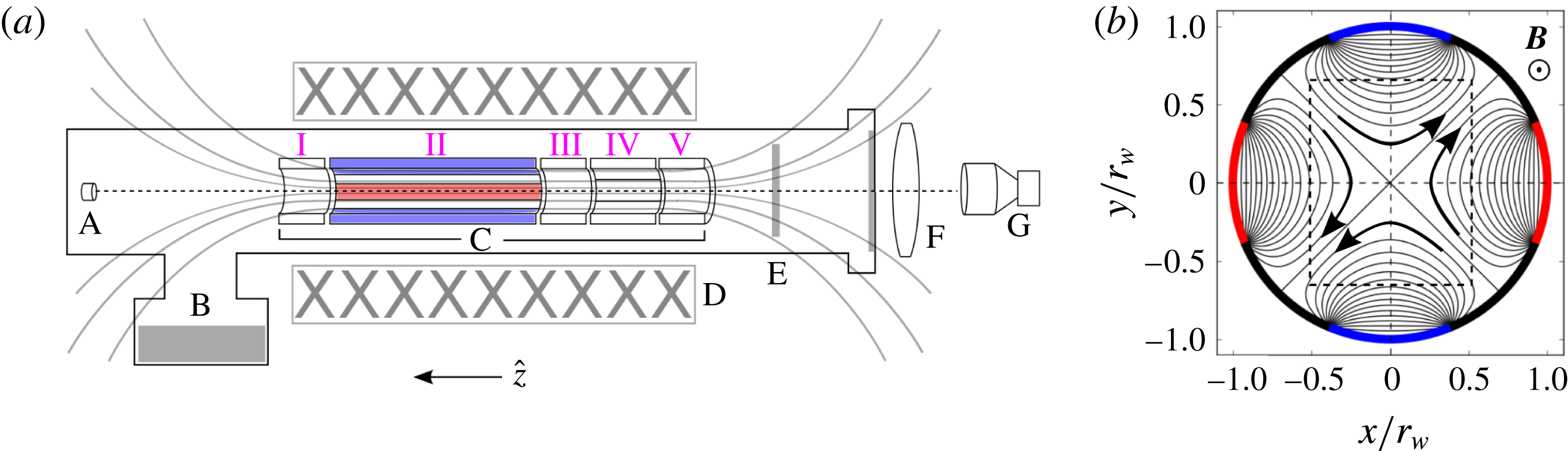
Components of the experimental apparatus are shown schematically in figure 3, including (a) a
 $(y,z)$
view perpendicular to the field, and (b) an
 $(x,y)$
view along the field. Solid electrodes I, III and V are used for axial confinement of electrons. Electrode IV is azimuthally segmented into four equal pieces. It is used for rotating wall plasma density profile control (Danielson et al.
Reference Danielson, Dubin, Greaves and Surko2015). Electrode II is divided azimuthally into eight equal segments. Electron plasmas are confined under electrode II for the fluid experiments described here, enabling the imposition of asymmetric boundary conditions. The entire electrode structure is 430 mm long, and electrode II is 260 mm long. A cryogenic pump maintains an ultra-high vacuum with pressure approximately
 $10^{-9}$
Torr inside a vacuum chamber which is shown in figure 3 as a solid black boundary. The electrodes are immersed in an axial magnetic field which is approximately uniform (
 $\unicode[STIX]{x1D6FF}B/B\lesssim 0.01$
) at
 $B=4.8$
T, shown schematically in figure 3 as black lines. It is generated by superconducting coils outside the vacuum chamber. For these experiments, typical plasma conditions are total electron number
 $N=1.5{-}7.2\times 10^{8}$
, central density
 $n_{0}=0.27{-}1.3\times 10^{14}~\text{m}^{-3}$
(corresponding to vorticity
 $\unicode[STIX]{x1D714}_{0}=100{-}500~\text{krad}~\text{s}^{-1}$
) and temperature
 $T\approx 0.1$
eV.
Schematic diagram of 8ST apparatus. (a)
 $(y,z)$
view of the 8ST apparatus, including electron source (A), cryo-pump (B), 8ST electrodes (C), magnet coils (D), phosphor screen (E), optical lens (F) and CCD camera (G). Magnetic field lines are shown schematically, as is the vacuum chamber enclosing the electrodes. (b)
 $(x,y)$
view of the 8-segment electrodes, including streamlines of the
 $\boldsymbol{E}\times \boldsymbol{B}$
flow (black lines) due to boundary potentials
 $+V_{s}$
(red) and
 $-V_{s}$
(blue), and a box (dashed) corresponding to the panels in figure 1.

2.2.2 Applied strain flow
The applied potential used for the fluid experiments is shown in figure 3(b) as black contours; they are the analogue of fluid streamlines, with flow direction specified by the arrows. The eight segments of electrode II are biased to voltages
 $V_{s}(1,0,-1,0,1,0,-1,0)$
, starting with the electrode aligned with the positive
 $x$
-axis. This pattern is used exclusively in the work described here, although the magnitude of
 $V_{s}$
is varied. The applied potential due to these boundary conditions,
 $$\begin{eqnarray}\displaystyle \unicode[STIX]{x1D719}_{s}(r,\unicode[STIX]{x1D703})=\mathop{\sum }_{m=0}^{\infty }A_{m}\left(\frac{r}{r_{w}}\right)^{m}\cos (m\unicode[STIX]{x1D703}), & & \displaystyle\end{eqnarray}$$
is the solution to the Laplace equation
 $\unicode[STIX]{x1D6FB}^{2}\unicode[STIX]{x1D719}_{s}=0$
, with expansion coefficients
 $A_{m}$
and azimuthal wavenumber
 $m$
. Since the vorticity in the plasma/fluid correspondence is analogous to electron density, the fluid flow associated with the vacuum potential
 $\unicode[STIX]{x1D719}_{s}$
is necessarily irrotational. For the boundary conditions described above, the lowest non-zero coefficients are found to be
 $A_{2}\approx 0.9V_{s}$
and
 $A_{6}\approx 0.3V_{s}$
, so that near the axis of the domain
 $(r/r_{w}\ll 1)$
, the second-order term dominates. The drift velocity due to the second-order potential
 $\unicode[STIX]{x1D719}_{s}^{(2)}$
is
 $$\begin{eqnarray}\displaystyle \boldsymbol{v}_{\boldsymbol{s}}^{\boldsymbol{(2)}}=\frac{2A_{2}V_{s}}{Br_{w}^{2}}(y\hat{\boldsymbol{x}}+x\hat{\boldsymbol{y}}), & & \displaystyle\end{eqnarray}$$
which is called a ‘simple strain flow’, with the strain magnitude given by
 $$\begin{eqnarray}\displaystyle \unicode[STIX]{x1D716}=\frac{2A_{2}V_{s}}{Br_{w}^{2}}. & & \displaystyle\end{eqnarray}$$
The electrode geometry and magnetic field are fixed, so the applied strain magnitude
 $\unicode[STIX]{x1D716}$
may be controlled simply by adjusting the voltage
 $V_{s}$
applied to the eight-segment electrodes. The time dependence of the applied strain
 $\unicode[STIX]{x1D716}(t)$
is chosen by programming a waveform generator to produce the corresponding voltage
 $V_{s}(t)$
. In this way, an arbitrary time dependence can be chosen for the applied strain, subject to low-pass filtering from the electrode circuit on a time scale
 ${\sim}1~\unicode[STIX]{x03BC}\text{s}$
. In the work reported here, we focus on two relatively simple cases: a square pulse, where
 $V_{s}=V_{0}$
for
 $0<t<t_{f}$
, and a linear ramp, where
 $V_{s}(t)=V_{0}t/t_{f}$
, with
 $V_{0}=\text{constant}$
.
2.2.3 Preparation of the initial vorticity distribution
Prior to application of the strain flow, the plasma is prepared according to a protocol such that its properties (electron density, spatial distribution and temperature) are suitable for vortex experiments. First, the plasma is generated by trapping electrons between electrodes I and V using the electron source, and axial confinement voltages
 $V_{c}=-100$
V. The plasma is typically initiated with a low-amplitude
 $m=1$
diocotron mode (Danielson et al.
Reference Danielson, Dubin, Greaves and Surko2015), meaning that the plasma is offset from the cylindrical electrode axis and therefore executes a circular orbit due to its image field. This mode is eliminated using a feedback damping circuit connected to two segments of electrode II so the vortex is centred on the origin. Next, electrode IV is used to condition the plasma density profile via the rotating wall technique (Danielson et al.
Reference Danielson, Dubin, Greaves and Surko2015) in order to achieve the desired axisymmetric vorticity distribution. Then, the plasma is ‘cut’ by ramping electrode III to
 $-$
100 V; this results in two separate plasmas confined under electrodes II and IV. The plasma under electrode IV is discarded by grounding electrode V. This cutting process can also generate a small diocotron mode in the plasma remaining under electrode II, which is then damped again. Finally, the plasma under electrode II is allowed to cool via cyclotron radiation in the magnetic field (O’Neil Reference O’Neil1980) to roughly
 $T\approx 0.1$
eV, at which point the plasma obeys the separation of scales discussed in § 2.1 and can therefore be described by (1.2).
2.2.4 Fluid experiment
The fluid experiment begins with an axisymmetric electron density distribution
 $n(r)$
centred on the cylindrical electrode axis, confined between electrodes I and III. At
 $t=0$
, an external strain flow is generated by adjusting the voltage
 $V_{s}$
on four segments of electrode II, as described above (cf. figure 3
b), and the plasma density distribution evolves in response to the strain according to (1.2). At
 $t=t_{f}$
,
 $V_{s}$
is reduced to zero, and the
 $z$
-averaged plasma density
 $\langle n\rangle _{z}$
is destructively diagnosed by grounding electrode III and allowing the plasma to stream along the magnetic field onto the phosphor screen, which is biased to
 $+$
5 kV. The resulting fluorescent light passes through a window in the vacuum chamber. It is focused by a lens onto a CCD camera, and the data are recorded. After the run, a ‘dark’ CCD exposure is taken without plasma, and subtracted from the original image to eliminate background noise. The entire run cycle is repeated many times to generate data sets. For example,
 $t_{f}$
can be varied to acquire time series data.
A plasma subject to the simple strain flow (2.3) can be unstable to uniform translation away from the origin (Fajans, Backhaus & Gilson Reference Fajans, Backhaus and Gilson2000). This mode is stabilized by the diocotron rotation due to image charges induced in the wall when the diocotron frequency exceeds the strain rate,
 $4\unicode[STIX]{x03C0}\unicode[STIX]{x1D716}^{\ast }(r_{v}/r_{w})^{-2}<1$
, although this condition is rarely satisfied in these experiments. Care is taken to properly centre the initial vortex at the origin so as to delay the onset of the translational instability. For the experiments discussed here,
 $t_{f}\lesssim 50~\unicode[STIX]{x1D714}_{0}^{-1}$
and the vortex displacement does not exceed approximately
 $0.2r_{w}$
.
2.2.5 Data analysis
The result of a single run cycle is a 2-D array of integers corresponding to the light signal acquired by the CCD, which is proportional to vorticity
 $\unicode[STIX]{x1D714}(x,y)$
. The spatial resolution is 29.6 pixels/mm, and the signal-to-noise ratio (at peak vorticity) typically ranges from 20–100. Once acquired, the CCD image for each run is analysed. The streamfunction
 $\unicode[STIX]{x1D713}$
is calculated from the CCD data by solving the Poisson equation using a finite-difference method with the appropriate boundary conditions. The streamfunction is then differentiated numerically to obtain the velocity field, and differentiated again to find the strain tensor and the Okubo–Weiss parameter across the domain (Weiss Reference Weiss1991). Critical points of the system, defined by
 $\boldsymbol{v}=\mathbf{0}$
, are found from the velocity magnitude by using a local minimization routine. The total circulation
 $\unicode[STIX]{x1D6E4}$
is found by integrating the CCD signal over the domain,
 $\unicode[STIX]{x1D6E4}=\int \unicode[STIX]{x1D714}\,\text{d}A$
. The initial vorticity profile
 $\unicode[STIX]{x1D714}(r)$
is found by taking an azimuthal average,
 $\unicode[STIX]{x1D714}(r)=(2\unicode[STIX]{x03C0})^{-1}\int \unicode[STIX]{x1D714}\,\text{d}\unicode[STIX]{x1D703}$
, and the equation
 $$\begin{eqnarray}\displaystyle \unicode[STIX]{x1D714}(r)=\unicode[STIX]{x1D714}_{0}\exp \left[-\left(\frac{r}{r_{v}}\right)^{\unicode[STIX]{x1D6FC}}\right] & & \displaystyle\end{eqnarray}$$
is fit to the experimental profile using a least-squares routine where the peak vorticity
 $\unicode[STIX]{x1D714}_{0}$
, the vortex radius
 $r_{v}$
and the smoothness exponent
 $\unicode[STIX]{x1D6FC}$
are fit parameters.
This work focuses on elliptical distortions of the vortex core, described by an aspect ratio
 $\unicode[STIX]{x1D706}$
and orientation with respect to the strain axis
 $\unicode[STIX]{x1D709}$
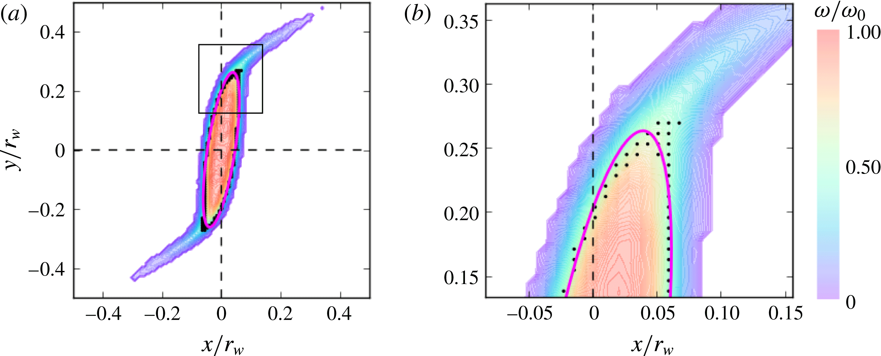
, and so these quantities must be extracted from the vorticity data. This is accomplished by using a least-squares routine to fit an ellipse to the half-maximum vorticity contour. In this way, low-vorticity filamentary structures do not influence the fit, and a robust representation of elliptical distortions of the vortex core is obtained. An example of an elliptical fit is shown in figure 4, corresponding to the data in the fourth panel of figure 1(b). Pixels with
 $0.4\leqslant \unicode[STIX]{x1D714}/\unicode[STIX]{x1D714}_{0}\leqslant 0.6$
are shown as black dots, and the ellipse (magenta line) is fit to these points. Panel (b) shows a zoomed-in region corresponding to the black square in panel (a), where the half-maximum contour diverges slightly from the elliptical shape due to filamentation.
Demonstration of the elliptical fitting routine. (a) Vorticity data from the fourth panel of figure 1(b); (b) zoomed-in region corresponding to black square in panel (a). Pixels with vorticity between
 $0.4\unicode[STIX]{x1D714}_{0}$
and
 $0.6\unicode[STIX]{x1D714}_{0}$
are shown as black dots. The ellipse (magenta line) is fitted to these points.

In order to compare the experimental
 $(\unicode[STIX]{x1D706},\unicode[STIX]{x1D709})$
values to theory, the finite diagnosis time for electrons to exit the trap and impinge on the phosphor screen must be accounted for. This may take a few microseconds. Over this time, the plasma continues to freely rotate (under zero external strain), leading to a shift in orientation
 $\unicode[STIX]{x0394}\unicode[STIX]{x1D709}$
. This shift is determined experimentally and subtracted from the data in order to obtain
 $\unicode[STIX]{x1D709}(t_{f})$
when the external strain is turned off.
One goal of this work is to study how the vortex dynamics is modified as the smoothness of the profile is varied. Therefore it is important to have precise control over the initial vorticity profile
 $\unicode[STIX]{x1D714}(r)$
. This is achieved using the rotating wall technique (Danielson et al.
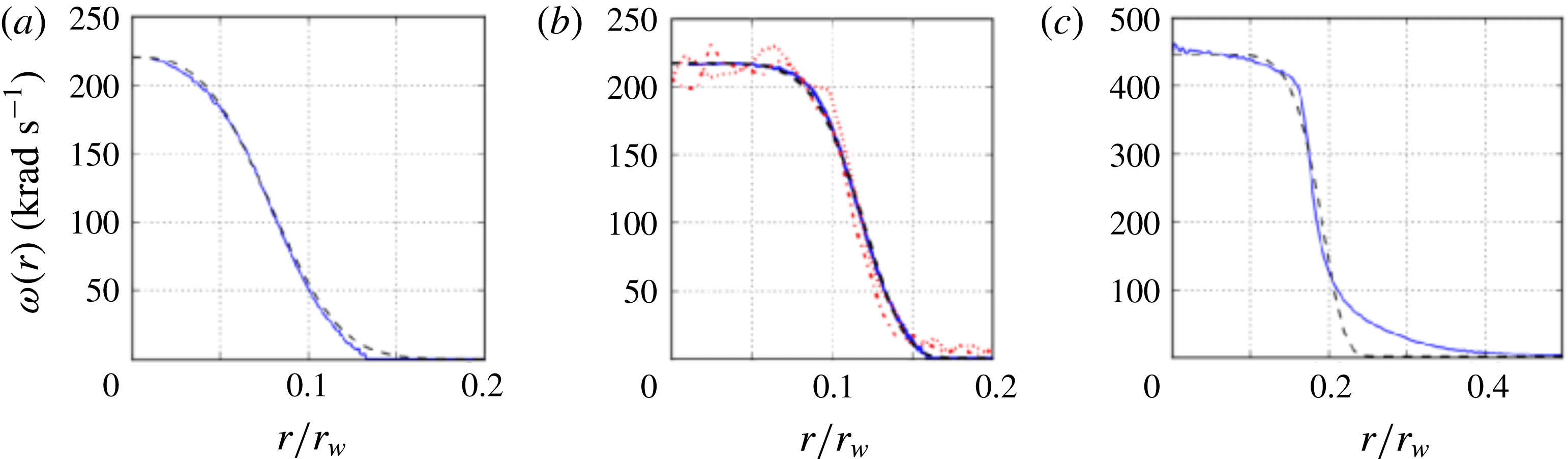
Reference Danielson, Dubin, Greaves and Surko2015), where oscillating electric potentials applied to electrode IV are implemented to drive radial transport of the electrons. Examples of initial vorticity profiles generated in this manner are shown in figure 5, including azimuthally averaged experimental data (solid lines) and fits to (2.5) (dashed). Shown are (a) a smooth profile with
 $\unicode[STIX]{x1D6FC}=3$
, (b) a quasi-flat profile with
 $\unicode[STIX]{x1D6FC}=6$
including vertical and horizontal slices of the CCD data and (c) a quasi-flat profile with
 $\unicode[STIX]{x1D6FC}\approx 8$
. In the case of figure 5(c), equation (2.5) is not a good fit due to a tail to the vorticity distribution at large radii. Once the desired profile has been obtained, the rotating wall potential is turned off, and the profile is stable (cf. figure 6). The total circulation can be adjusted during the plasma fill process by varying the number of trapped electrons. Smoothness exponents in the range
 $2\leqslant \unicode[STIX]{x1D6FC}\leqslant 10$
(cf. (2.5)) are used for the data reported here. The initial profiles produced by the rotating wall are axisymmetric to a high degree of precision. Elliptical fits to the initial profiles typically yield
 $\unicode[STIX]{x1D706}\approx 1.01$
, although this measurement is limited by the finite pixel size.
Examples of initial vorticity profiles obtained using the rotating wall technique, including data (blue, solid) and fits to (2.5) (black, dashed). (a) A smooth profile with
 $\unicode[STIX]{x1D6FC}=3$
; (b) a quasi-flat profile with
 $\unicode[STIX]{x1D6FC}=6$
, including vertical (red, dotted) and horizontal (red, dash-dot) slices; and (c) a quasi-flat profile with
 $\unicode[STIX]{x1D6FC}\approx 8$
, where the fit fails to capture a tail at the edge of the vorticity distribution.

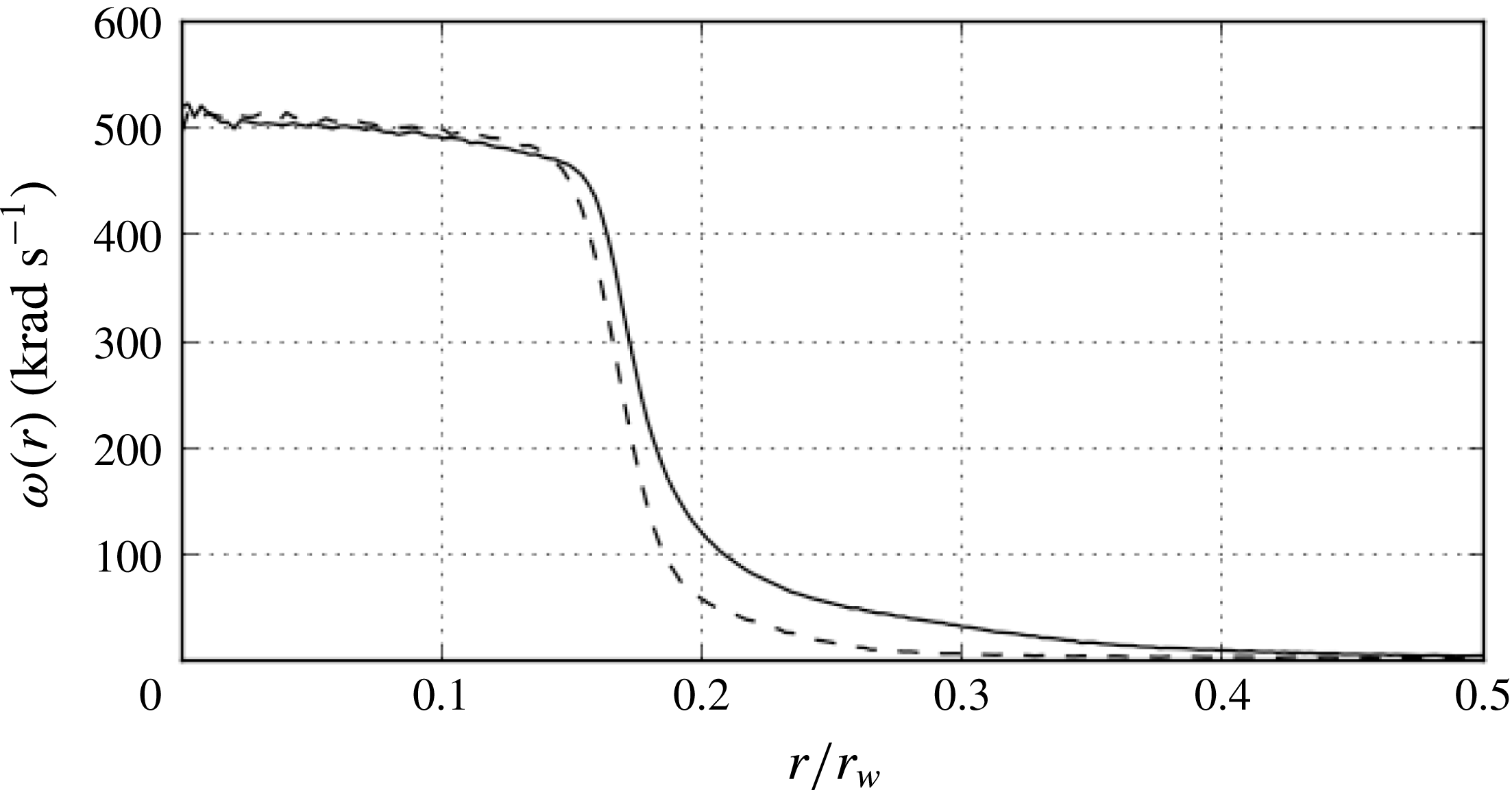
Stability of a freely relaxing vorticity profile. Shown are the initial profile (solid line) and the same profile after 10 s (
 $5\times 10^{6}\unicode[STIX]{x1D714}_{0}^{-1}$
) of evolution with
 $V_{s}=0$
(dashed).

2.2.6 Calibration
The vorticity is calibrated with the CCD light signal using a quasi-flat vortex (
 $\unicode[STIX]{x1D6FC}\geqslant 5$
) briefly excited to a small aspect ratio,
 $\unicode[STIX]{x1D706}\approx 1.2$
, by the external strain. In this case, the rotation rate is
 $\text{d}\unicode[STIX]{x1D709}/\text{d}t\approx \unicode[STIX]{x1D714}/4$
(Saffman Reference Saffman1992). The vorticity is measured using the elliptical fitting routine to extract
 $\unicode[STIX]{x1D709}(t)$
. The strain magnitude can be calculated directly from the electrode geometry, the magnetic field and the applied voltage using (2.4); however, it can also be independently calibrated using a rapid distortion technique. Here, a constant strain is applied with
 $\unicode[STIX]{x1D716}^{\ast }\approx 0.25$
. In this case, the strain is sufficiently strong that the vorticity behaves passively and the aspect ratio evolves as
 $$\begin{eqnarray}\displaystyle \unicode[STIX]{x1D706}(t)\approx \exp (2\unicode[STIX]{x1D716}t). & & \displaystyle\end{eqnarray}$$
This is repeated varying
 $\unicode[STIX]{x1D716}^{\ast }$
, and
 $\unicode[STIX]{x1D706}(t)$
is diagnosed in order to verify that the assumption of passive vorticity is valid. Results of this technique disagree slightly with the strain magnitude calculated from (2.4). The calibrated strain magnitude (determined from fitting data to (2.6)) is used for all data presented here. This discrepancy and further details of the calibration process are discussed elsewhere (Hurst et al.
Reference Hurst, Danielson and Surko2018).
2.2.7 Limitations to the plasma/fluid analogy
It is important to understand how the plasma/fluid analogy is broken when the spatio-temporal scale separations described in § 2.1 are not satisfied. The conditions
 $f_{g}\gg f_{v}$
and
 $r_{g}\ll r_{v}$
are related to the finite size and internal structure of the electron point vortices; they are satisfied by many orders of magnitude in the 8ST due to the strong magnetic field. The condition
 $r_{w}\ll L$
is related to 3-D effects due to the endcap confinement potentials, which give rise to a background rotation called the ‘magnetron drift’ (Danielson et al.
Reference Danielson, Dubin, Greaves and Surko2015). In the 8ST,
 $L/r_{w}=20$
, and the magnetron frequency is approximately three orders of magnitude lower than
 $f_{v}$
. The condition
 $f_{b}\gg f_{v}$
is related to the rigidity of the electron line charges; when this is violated, 3-D effects are expected which could give rise to a smearing of the point vortices. Additionally, smearing effects are expected from temperature-dependent magnetron drifts (Peurrung & Fajans Reference Peurrung and Fajans1993). In the 8ST, sharp vorticity features are routinely observed, and no evidence of smearing is apparent.
The condition
 $f_{v}\gg f_{c}$
ensures that viscous effects can be neglected. This is satisfied by at least an order of magnitude in the 8ST. The plasma viscosity arises from like-particle collisions between magnetized electrons. Thus, where the electron density is zero (i.e. in irrotational regions of the flow), the viscosity is identically zero; and in general, the viscosity varies with electron density inside the plasma. Therefore, the plasma viscosity differs fundamentally from that of a traditional hydrodynamic system, where viscosity is approximately uniform throughout. Thus, viscous effects are outside the scope of the plasma/fluid analogy. Since the plasma is isolated from the wall, the fluid obeys free-slip boundary conditions. Radial transport of the vorticity under symmetric boundary conditions is slow. Figure 6 shows a quasi-flat vortex which remains approximately static over time
 $10^{6}\unicode[STIX]{x1D714}_{0}^{-1}$
, thus defining an effective Reynolds number of
 $Re>10^{6}$
. Further information on viscosity and radial transport in electron plasmas can be found in Kriesel & Driscoll (Reference Kriesel and Driscoll2000) and Kriesel & Driscoll (Reference Kriesel and Driscoll2001).
2.3 Vortex-in-cell simulations
To support and extend the 8ST experimental results, numerical simulations are conducted using the vortex-in-cell technique (Leonard Reference Leonard1980). The vorticity distribution is approximated by a number of discrete point vortices of equal strength. A Monte Carlo method is used to arrange the point vortices to achieve the desired initial profile given by (2.5). Alternatively, experimentally measured vorticity profiles can be loaded into the simulation. At each time step, the Poisson equation is solved on a grid using a finite-difference method, subject to the same boundary conditions used in the experiments (see figure 3
b). The streamfunction at the location of each point vortex is calculated using a linear interpolation between grid points, and time is advanced using a fourth-order Runge–Kutta technique. Typical simulation parameters are the number of point vortices
 $N\sim 10^{5}$
, 300 grid points in the wall diameter and a time step
 ${\sim}0.05\unicode[STIX]{x1D714}_{0}^{-1}$
. The displacement of the entire vorticity distribution is feedback-damped artificially in the simulation in order to avoid translation instability due to the external strain, thus allowing for longer time scales than are possible in the experiments.
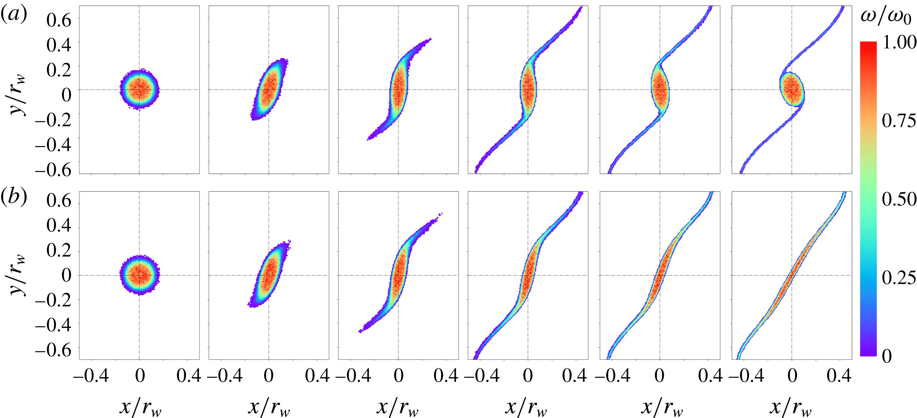
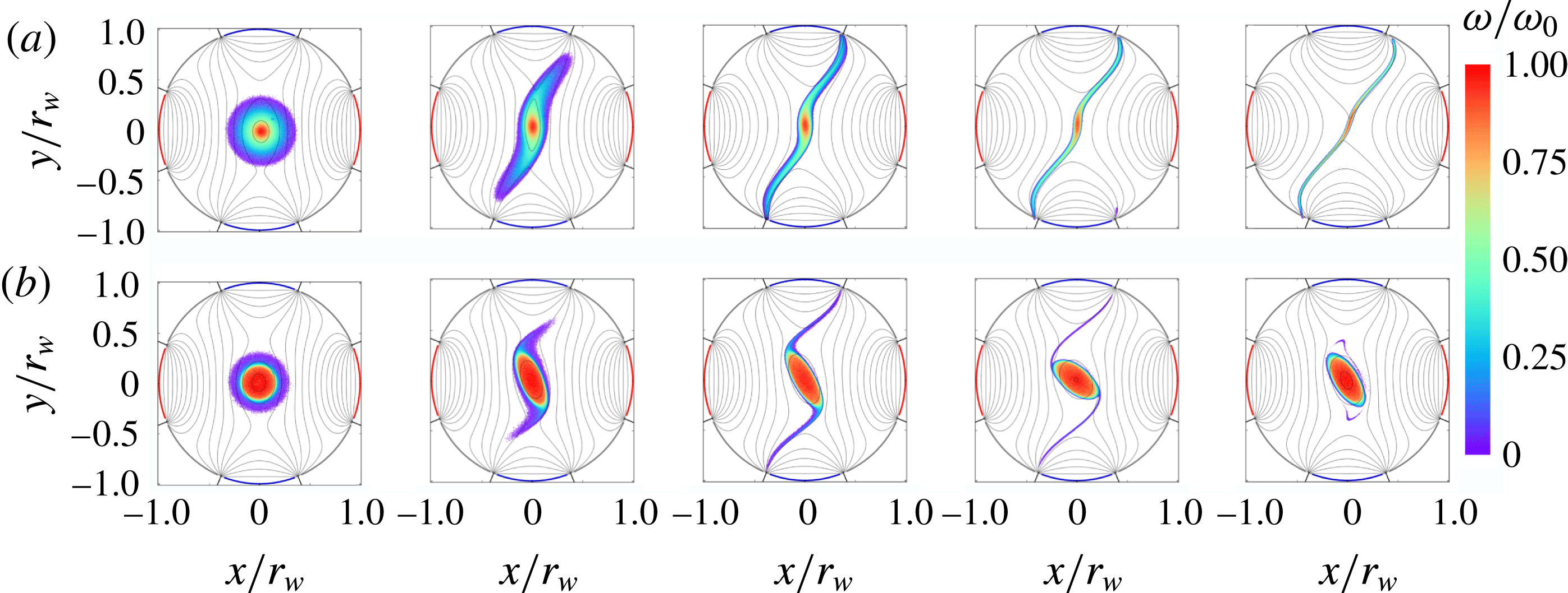
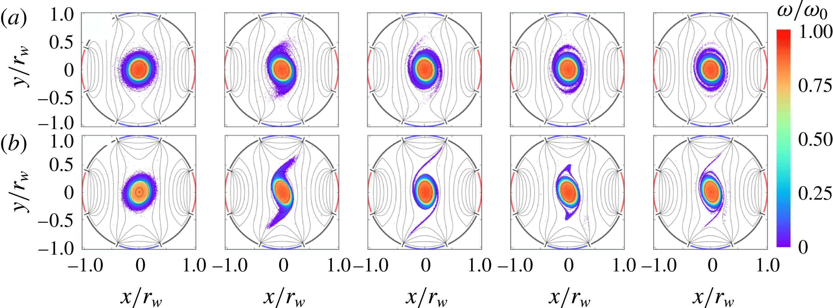
Examples of the results of vortex-in-cell simulations are shown in figure 7, corresponding directly to the data in figure 1, with (a)
 $\unicode[STIX]{x1D716}^{\ast }=0.116$
and (b)
 $\unicode[STIX]{x1D716}^{\ast }=0.13$
. The simulation results in figure 7 are in good qualitative agreement with the experimental results in figure 1. Notable differences are that the experimental vortices are rotated counter-clockwise slightly due to the diagnosis process, and the thin filaments are more difficult to observe in the laboratory due to noise acquired by the CCD.
Vortex-in-cell simulations of strained quasi-flat vortices with applied strain (a)
 $\unicode[STIX]{x1D716}^{\ast }=0.116$
and (b)
 $\unicode[STIX]{x1D716}^{\ast }=0.13$
and
 $0\leqslant t\leqslant 22.8\unicode[STIX]{x1D714}_{0}^{-1}$
. These results correspond directly to the experimental data in figure 1.

3 Theoretical description of strained vortices
Ideal 2-D fluids are described by the 2-D Euler equations (1.1). The flow field is uniquely specified by the vorticity and the boundary conditions via the Poisson equation,
 $\unicode[STIX]{x1D6FB}^{2}\unicode[STIX]{x1D713}=\unicode[STIX]{x1D714}$
. Equations (1.1) form a continuous Hamiltonian system, where the vorticity is locally conserved in the Lagrangian frame (Morrison Reference Morrison1998). The dissipationless flow also conserves internal energy along streamlines, so thermal forces are absent and the pressure can be calculated directly from the flow field (Majda & Bertozzi Reference Majda and Bertozzi2002). The streamfunction can be decomposed into homogeneous and particular solutions,
 $\unicode[STIX]{x1D713}=\unicode[STIX]{x1D713}_{s}+\unicode[STIX]{x1D713}_{v}$
where
 $\unicode[STIX]{x1D713}_{s}$
describes irrotational flow associated with boundary conditions and
 $\unicode[STIX]{x1D713}_{v}$
describes flow generated by the vorticity.
A key theme in the present work is the competition between strain and vorticity in a 2-D fluid. The velocity gradient tensor at any point
 $\unicode[STIX]{x1D735}\boldsymbol{v}(x,y,t)$
can be decomposed into its symmetric part
 $\unicode[STIX]{x1D748}\equiv (1/2)[\unicode[STIX]{x1D735}\boldsymbol{v}+(\unicode[STIX]{x1D735}\boldsymbol{v})^{\text{T}}]$
which is called the strain tensor, and its antisymmetric part
 $\unicode[STIX]{x1D734}\equiv (1/2)[\unicode[STIX]{x1D735}\boldsymbol{v}-(\unicode[STIX]{x1D735}\boldsymbol{v})^{\text{T}}]$
which is called the vorticity tensor. The vorticity tensor has complex conjugate eigenvalues with magnitude equal to the vorticity
 $\unicode[STIX]{x1D714}$
in the
 $\hat{\boldsymbol{z}}$
direction. Assuming incompressibility, the strain tensor is traceless with real eigenvalues
 $\pm s=\pm [4\unicode[STIX]{x1D713}_{xy}^{2}+(\unicode[STIX]{x1D713}_{xx}-\unicode[STIX]{x1D713}_{yy})^{2}]^{1/2}$
where subscripts indicate partial derivatives. The magnitude of the strain and vorticity eigenvalues can be combined to form a dimensionless parameter
 $s^{\ast }=|s/\unicode[STIX]{x1D714}|$
, which quantifies the local competition between strain and vorticity, with
 $s^{\ast }\gg 1$
corresponding to strain-dominated hyperbolic fluid motion and
 $s^{\ast }\ll 1$
corresponding to vorticity-dominated periodic fluid motion.
Here we consider an initially axisymmetric, monotonically decreasing vorticity distribution
 $\unicode[STIX]{x1D714}(r)$
in a 2-D ideal fluid, subject to an externally imposed irrotational simple strain flow defined by (1.3). The external strain flow
 $\unicode[STIX]{x1D713}_{s}$
has a uniform strain tensor everywhere, where the eigenvalue is
 $s=2\unicode[STIX]{x1D716}$
and the strain axis orientation (i.e. the direction of the positive eigenvector) is
 $\unicode[STIX]{x03C0}/4$
. However,
 $s$
may vary across the domain when the full flow field
 $\unicode[STIX]{x1D713}=\unicode[STIX]{x1D713}_{s}+\unicode[STIX]{x1D713}_{v}$
is considered, since
 $\unicode[STIX]{x1D713}_{v}$
can contribute to the strain tensor.
A goal of this work is to study the behaviour of quasi-flat radial vorticity profiles, where
 $\unicode[STIX]{x1D714}(r)$
is a constant in the core, and then decreases quickly to zero at the edge of the vortex (cf. figure 5
b). When the vorticity gradient is very steep, elliptical vortex patch theory is expected to be an accurate description. Another goal is to study how the dynamics depends on the degree of flatness of the profile. When the profile is relatively smooth (cf. figure 5
a), departures from the elliptical patch theory are expected. In this section, details of the vortex patch model and its predictions are presented, then theoretical efforts regarding smooth profiles are discussed. Theoretical results are compared to experimental and numerical data in § 4.
3.1 Elliptical patch model
A particularly useful theoretical description of 2-D ideal vortices is the so-called elliptical patch model, where the vorticity is treated as piecewise-constant with vorticity
 $\unicode[STIX]{x1D714}_{0}$
inside an elliptical boundary and zero elsewhere. Neglecting uniform translations and imposing incompressibility, the ellipse can be described by the aspect ratio
 $\unicode[STIX]{x1D706}\equiv a/b$
and the orientation
 $\unicode[STIX]{x1D709}$
, where
 $a$
and
 $b$
are the semimajor and semiminor axes. In the absence of external flow, Kirchoff found that the patch rotates freely with
 $\text{d}\unicode[STIX]{x1D706}/\text{d}t=0$
and (Saffman Reference Saffman1992)
 $$\begin{eqnarray}\displaystyle \frac{\text{d}\unicode[STIX]{x1D709}}{\text{d}t}=\unicode[STIX]{x1D714}_{0}\frac{\unicode[STIX]{x1D706}}{(\unicode[STIX]{x1D706}+1)^{2}}. & & \displaystyle\end{eqnarray}$$
In the presence of the time-independent simple strain flow (1.3), the behaviour of the elliptical vortex patch was solved exactly by K81 (Kida Reference Kida1981). Dynamical equations for the aspect ratio and orientation are given by
 $$\begin{eqnarray}\displaystyle & \displaystyle \frac{\text{d}\unicode[STIX]{x1D706}}{\text{d}t}=2\unicode[STIX]{x1D706}\unicode[STIX]{x1D716}\cos 2\unicode[STIX]{x1D709}, & \displaystyle\end{eqnarray}$$
 $$\begin{eqnarray}\displaystyle & \displaystyle \frac{\text{d}\unicode[STIX]{x1D709}}{\text{d}t}=-\unicode[STIX]{x1D716}\sin 2\unicode[STIX]{x1D709}\frac{\unicode[STIX]{x1D706}^{2}+1}{\unicode[STIX]{x1D706}^{2}-1}+\unicode[STIX]{x1D714}_{0}\frac{\unicode[STIX]{x1D706}}{(\unicode[STIX]{x1D706}+1)^{2}}, & \displaystyle\end{eqnarray}$$
where
 $\unicode[STIX]{x1D709}$
is defined relative to the strain axis. These equations were solved by eliminating the time dependence and extracting trajectories of the form
 $$\begin{eqnarray}\displaystyle \unicode[STIX]{x1D716}\sin 2\unicode[STIX]{x1D709}=\unicode[STIX]{x1D714}_{0}\left[\frac{\unicode[STIX]{x1D706}}{\unicode[STIX]{x1D706}^{2}-1}\ln \frac{(\unicode[STIX]{x1D706}+1)^{2}}{4C\unicode[STIX]{x1D706}}\right], & & \displaystyle\end{eqnarray}$$
where
 $C$
is an integration constant associated with the initial condition, with
 $C=1$
corresponding to an initially circular vortex,
 $\unicode[STIX]{x1D706}(t=0)=1$
.
Since the Euler flow is dissipationless, the K81 system preserves total energy. The Hamiltonian
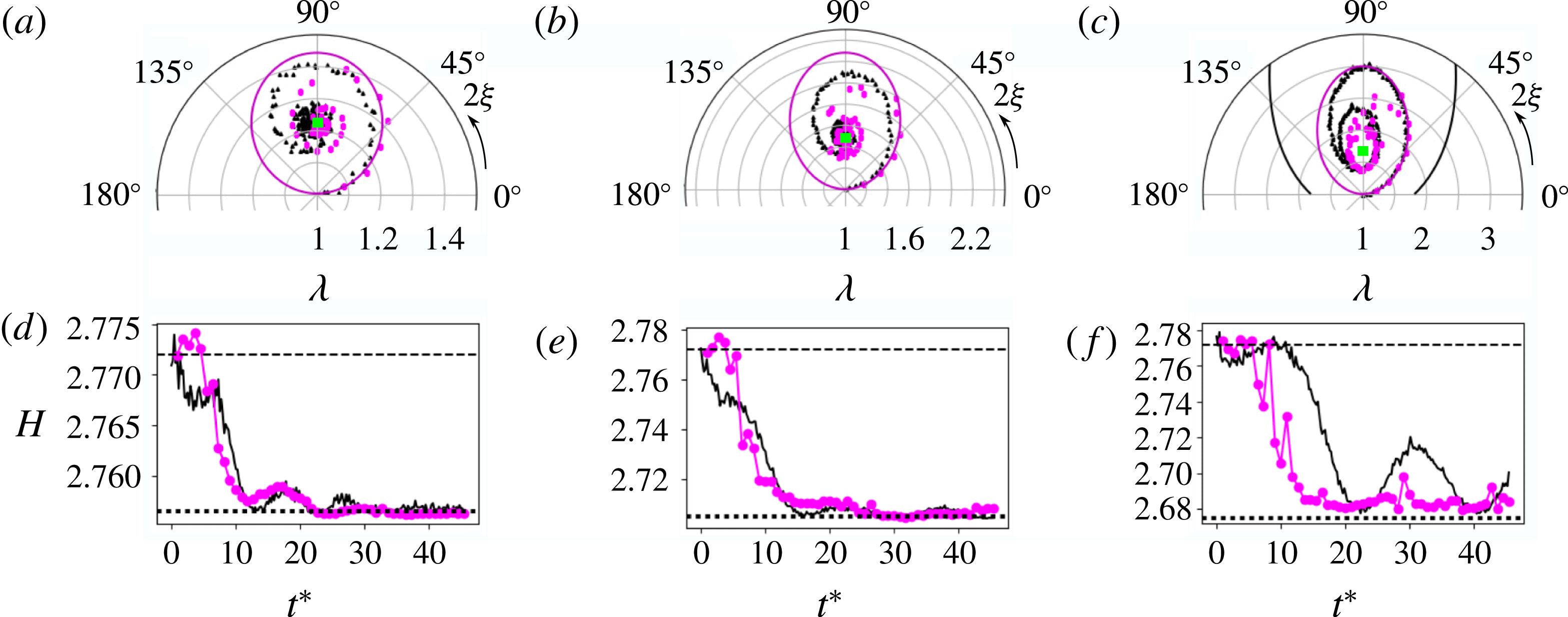
 $$\begin{eqnarray}\displaystyle H(\unicode[STIX]{x1D706},\unicode[STIX]{x1D709})=2\unicode[STIX]{x1D716}\sin 2\unicode[STIX]{x1D709}\frac{1-\unicode[STIX]{x1D706}^{2}}{\unicode[STIX]{x1D706}}+2\unicode[STIX]{x1D714}_{0}\ln \left[\frac{(1+\unicode[STIX]{x1D706})^{2}}{\unicode[STIX]{x1D706}}\right] & & \displaystyle\end{eqnarray}$$
is invariant along a trajectory in phase space (Meacham, Morrison & Flierl Reference Meacham, Morrison and Flierl1997), and
 $C=(1/4)\exp (H/2\unicode[STIX]{x1D714}_{0})$
. Although
 $(\unicode[STIX]{x1D706},\unicode[STIX]{x1D709})$
are physically intuitive quantities, they are not canonical coordinates for this system, and they are degenerate under the transformations
 $(\unicode[STIX]{x1D706},\unicode[STIX]{x1D709})\rightarrow (1/\unicode[STIX]{x1D706},\unicode[STIX]{x1D709}+\unicode[STIX]{x03C0}/2)$
and
 $\unicode[STIX]{x1D709}\rightarrow \unicode[STIX]{x1D709}+\unicode[STIX]{x03C0}$
. A suitable choice of canonical momentum and coordinate is (Melander, Zabusky & Styczek Reference Melander, Zabusky and Styczek1986)
 $$\begin{eqnarray}\displaystyle p=\frac{(\unicode[STIX]{x1D706}-1)^{2}}{\unicode[STIX]{x1D706}},\quad q=2\unicode[STIX]{x1D709}, & & \displaystyle\end{eqnarray}$$
yielding the Hamiltonian
 $$\begin{eqnarray}\displaystyle H(p,q)=-2\unicode[STIX]{x1D716}\sin q\sqrt{p^{2}+4p}+2\unicode[STIX]{x1D714}\ln (p+4). & & \displaystyle\end{eqnarray}$$
In this work, coordinates
 $(\unicode[STIX]{x1D706},\unicode[STIX]{x1D709})$
are used for most results to aid physical intuition, where
 $1\leqslant \unicode[STIX]{x1D706}$
and
 $0\leqslant \unicode[STIX]{x1D709}<\unicode[STIX]{x03C0}$
.
It is useful to normalize time to
 $\unicode[STIX]{x1D714}_{0}^{-1}$
, such that
 $t\rightarrow t^{\ast }=t\unicode[STIX]{x1D714}_{0}$
. The first term on the right-hand side of (3.5) is the interaction energy between the patch and the strain, and the second term is the self-energy associated with elliptical distortion of the patch (Vanneste & Young Reference Vanneste and Young2010) (note that the second term on the right-hand side of (3.3) is given by (3.1)). Thus the dynamics can be described qualitatively as a competition between the two terms in the Hamiltonian representing stretching and rotation of the patch, parameterized by
 $\unicode[STIX]{x1D716}^{\ast }\equiv \unicode[STIX]{x1D716}/\unicode[STIX]{x1D714}_{0}$
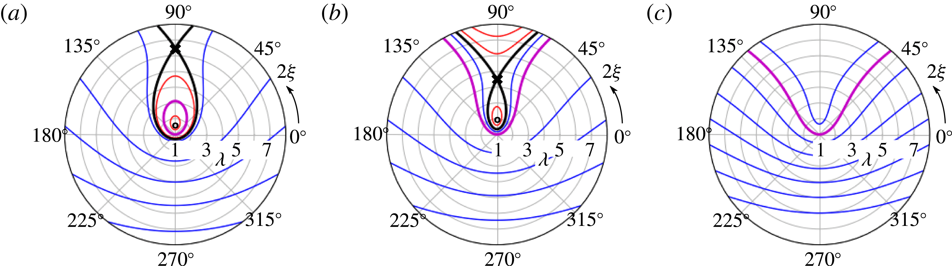
. Contours of the K81 Hamiltonian (3.5) are plotted in figure 8(a–c) for three values of the normalized strain parameter,
 $\unicode[STIX]{x1D716}^{\ast }=0.11,0.135,0.155$
.
Contours of the K81 Hamiltonian (3.5) in polar coordinates
 $(\unicode[STIX]{x1D706},2\unicode[STIX]{x1D709})$
for
 $\unicode[STIX]{x1D716}^{\ast }=$
(a) 0.11, (b) 0.135 and (c) 0.155, with saddle (centre) points shown as
 $X$
(
 $O$
), the separatrix (thick black line), closed orbits (red), open orbits (blue) and the orbit corresponding to
 $C=1$
(thick magenta line).

The behaviour of the K81 system is dictated by its fixed points
 $(\unicode[STIX]{x1D706}_{0},\unicode[STIX]{x1D709}_{0})$
, which are defined by
 $\text{d}\unicode[STIX]{x1D706}/\text{d}t=\text{d}\unicode[STIX]{x1D709}/\text{d}t=0$
, resulting in
 $\unicode[STIX]{x1D709}_{0}=\unicode[STIX]{x03C0}/4$
and
 $\unicode[STIX]{x1D706}_{0}$
given by the solution to
 $$\begin{eqnarray}\displaystyle \frac{\unicode[STIX]{x1D706}_{0}(\unicode[STIX]{x1D706}_{0}-1)}{(\unicode[STIX]{x1D706}_{0}+1)(\unicode[STIX]{x1D706}_{0}^{2}+1)}=\unicode[STIX]{x1D716}^{\ast }. & & \displaystyle\end{eqnarray}$$
This formula was first derived by MS71 (Moore & Saffman Reference Moore, Saffman, Rogers, Olsen and Goldburg1971), and later, independently, in the context of electron plasma by Backhaus, Fajans & Wurtele (Reference Backhaus, Fajans and Wurtele1999). For
 $\unicode[STIX]{x1D716}^{\ast }<\unicode[STIX]{x1D716}_{c}^{\ast }$
, equation (3.8) has two solutions, where
 $\unicode[STIX]{x1D716}_{c}^{\ast }\approx 0.15$
is the critical strain value. At
 $\unicode[STIX]{x1D716}_{c}^{\ast }$
the two branches meet, and above
 $\unicode[STIX]{x1D716}_{c}^{\ast }$
there are no solutions. For a given value of the parameter
 $\unicode[STIX]{x1D716}^{\ast }<\unicode[STIX]{x1D716}_{c}^{\ast }$
, the K81 phase space contains an unstable saddle point and a stable centre point corresponding to the upper and lower branches of (3.8), respectively. The saddle point defines a separatrix which divides the phase space into closed and open (i.e. stable and unstable) orbits. The centre point corresponds to a local minimum of
 $H$
. The fixed points and separatrices are shown graphically in figure 8.
Physically, a closed orbit not enclosing the origin corresponds to a nutation of the ellipse where
 $\unicode[STIX]{x1D709}$
is bounded, and one enclosing the origin corresponds to rotation of the ellipse where
 $\unicode[STIX]{x1D709}$
increases monotonically. The orbit with circular initial condition (
 $C=1$
) marks the boundary between rotations and nutations. These modes are generalizations of the linear vortex patch perturbations known as Kelvin waves (Saffman Reference Saffman1992), or diocotron waves in the context of non-neutral plasma (Danielson et al.
Reference Danielson, Dubin, Greaves and Surko2015). Open orbits correspond to destruction modes of the vortex; here,
 $\unicode[STIX]{x1D709}$
is bounded and
 $\unicode[STIX]{x1D706}$
is unbounded from above, and the vortex is stretched into an ever-thinning filament aligned with the strain axis.
An orbit is uniquely defined by the constant
 $C$
and the normalized strain
 $\unicode[STIX]{x1D716}^{\ast }$
. For a given value of
 $C$
, there exists a critical value of the strain called the dynamical stability limit
 $\unicode[STIX]{x1D716}_{d}^{\ast }(C)$
where the orbit coincides with the separatrix. The orbit is closed if
 $\unicode[STIX]{x1D716}^{\ast }<\unicode[STIX]{x1D716}_{d}^{\ast }$
or open if
 $\unicode[STIX]{x1D716}^{\ast }>\unicode[STIX]{x1D716}_{d}^{\ast }$
. The dynamical stability limit can be calculated by determining when the maximum value
 $\unicode[STIX]{x1D706}_{m}$
of the aspect ratio reached in the orbit coincides with the upper branch of (3.8). At this point,
 $\text{d}\unicode[STIX]{x1D706}/\text{d}t=0$
, yielding
 $\unicode[STIX]{x1D709}=\unicode[STIX]{x03C0}/4$
, and
 $\unicode[STIX]{x1D706}_{m}$
is given by the solution to
 $$\begin{eqnarray}\displaystyle \frac{\unicode[STIX]{x1D706}_{m}}{\unicode[STIX]{x1D706}_{m}^{2}-1}\ln \left[\frac{(\unicode[STIX]{x1D706}_{m}+1)^{2}}{4C\unicode[STIX]{x1D706}_{m}}\right]=\unicode[STIX]{x1D716}^{\ast }. & & \displaystyle\end{eqnarray}$$
When the left sides of (3.8) and (3.9) are equated and
 $C$
is specified, the solution for
 $\unicode[STIX]{x1D706}$
can be used to find the stability limit
 $\unicode[STIX]{x1D716}_{d}^{\ast }(C)$
. The case of circular initial condition (
 $C=1$
) is particularly important in this work since the 8ST produces initially axisymmetric vortices. In this case,
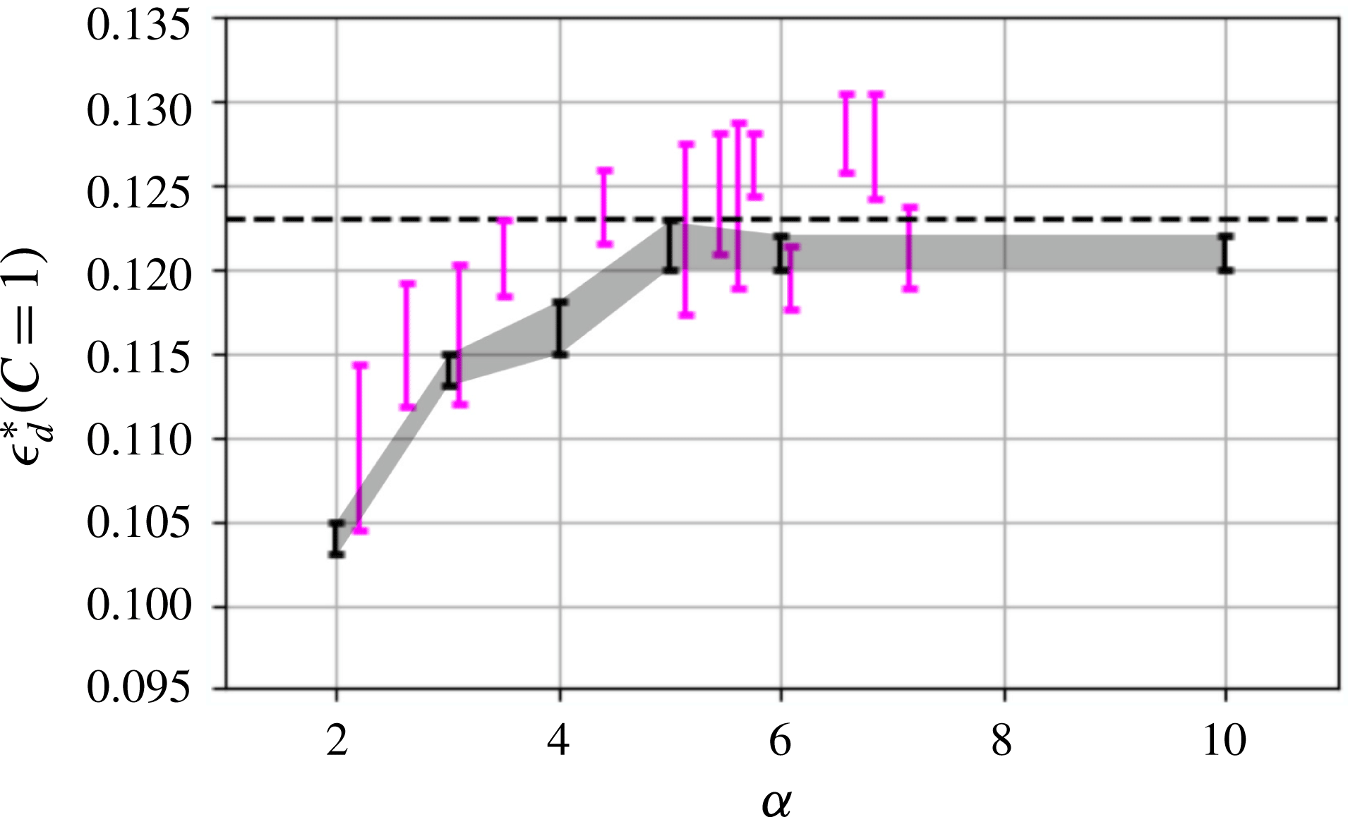
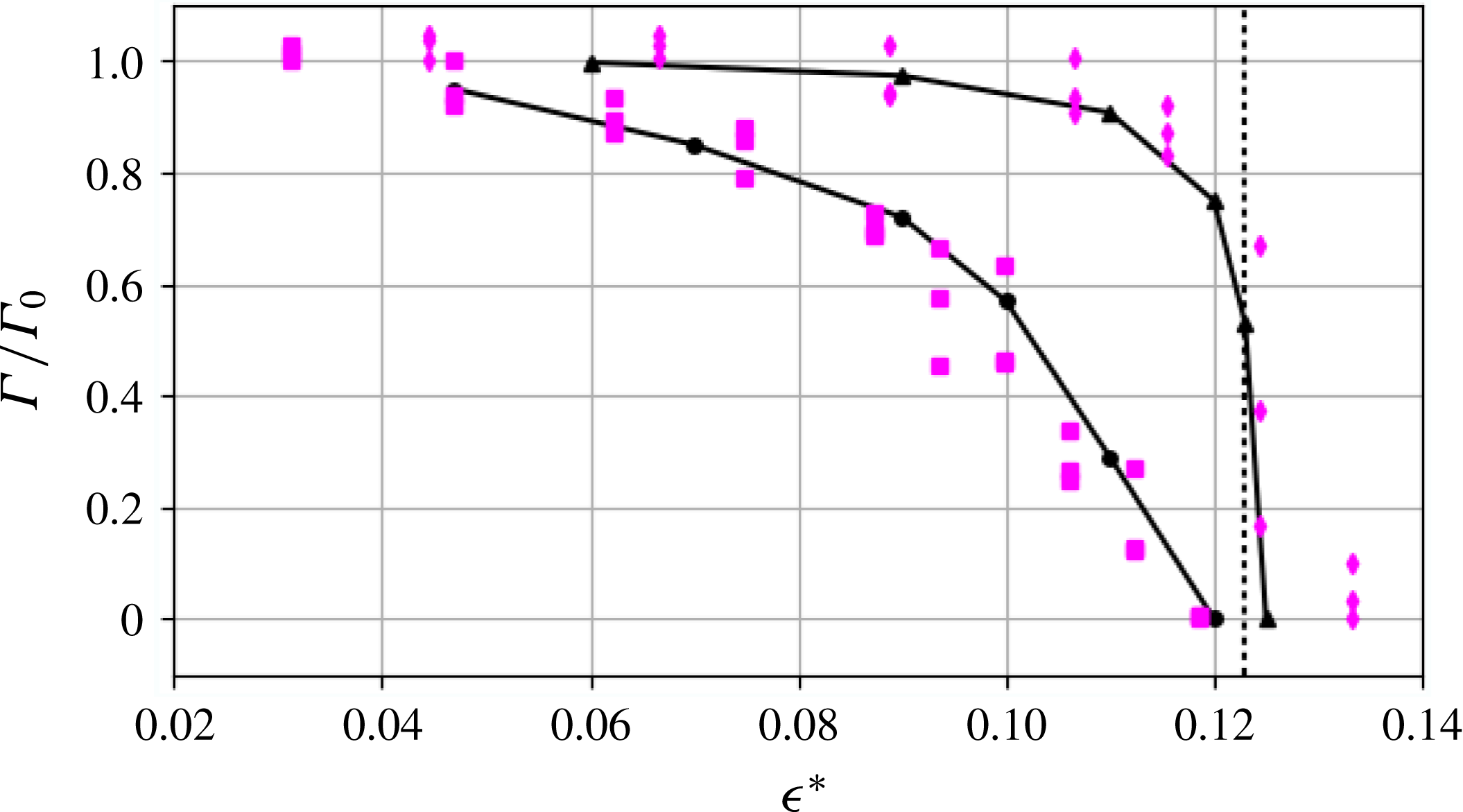
 $\unicode[STIX]{x1D716}_{d}^{\ast }\approx 0.123$
, which corresponds to
 $\unicode[STIX]{x1D706}_{m}\approx 5.4$
. Thus an initially circular vortex patch subject to constant strain is destroyed at a smaller value of strain than the equilibrium critical value
 $\unicode[STIX]{x1D716}_{c}^{\ast }\approx 0.15$
, and in general
 $\unicode[STIX]{x1D716}_{d}^{\ast }$
can vary with
 $C$
across the interval
 $(0,\unicode[STIX]{x1D716}_{c}^{\ast })$
. The strain values shown in figure 8 are chosen such that for the lowest (a)
 $\unicode[STIX]{x1D716}^{\ast }<0.123$
with
 $C=1$
corresponding to a closed orbit; then (b)
 $0.123<\unicode[STIX]{x1D716}^{\ast }<0.15$
where
 $C=1$
is an open orbit, and finally (c)
 $\unicode[STIX]{x1D716}^{\ast }>0.15$
where no fixed points exist and all orbits are open.
The K81 system can be simplified substantially by neglecting one of the two terms in the Hamiltonian. The rotation term always dominates when
 $\unicode[STIX]{x1D706}$
is near 1; however for
 $C=1$
with sufficiently large
 $\unicode[STIX]{x1D716}^{\ast }$
,
 $\text{d}\unicode[STIX]{x1D706}/\text{d}t\gg \text{d}\unicode[STIX]{x1D709}/\text{d}t$
and
 $\unicode[STIX]{x1D706}$
quickly grows to a value where the strain term dominates. In this case,
 $\unicode[STIX]{x1D709}(t)\approx 0$
, the rotation term is negligible, and the vorticity is advected like a passive scalar. Thus the solution to (3.2) is approximately given by (2.6). On the other hand, in the limit of small
 $\unicode[STIX]{x1D716}^{\ast }$
, the rotation term dominates over the strain and the orbits are simply perturbed Kelvin waves.
In this discussion so far, the normalized strain
 $\unicode[STIX]{x1D716}^{\ast }$
was defined as the ratio of the external strain magnitude to the vorticity of the patch. However, the vortex can produce localized strain as well. Based on the particular solution to the Poisson equation
 $\unicode[STIX]{x1D713}_{v}$
, an elliptical vortex patch produces a constant strain within the patch with eigenvalue
 $$\begin{eqnarray}\displaystyle s_{v}=\unicode[STIX]{x1D714}_{0}\left(\frac{\unicode[STIX]{x1D706}-1}{\unicode[STIX]{x1D706}+1}\right) & & \displaystyle\end{eqnarray}$$
and orientation
 $\unicode[STIX]{x1D709}-\unicode[STIX]{x03C0}/4$
. Therefore, the total strain
 $s=s_{v}+2\unicode[STIX]{x1D716}$
inside the elliptical vortex patch can be much larger than the applied strain. For example, a patch in equilibrium just below the threshold has
 $\unicode[STIX]{x1D716}^{\ast }\approx 0.15$
,
 $\unicode[STIX]{x1D706}\approx 2.9$
, and
 $s_{v}/2\approx 0.25$
, so the self-strain exceeds the applied strain significantly.
Another important point is that the K81 solutions described above are possible because an initially elliptical vortex patch remains elliptical at all times under the action of a simple strain flow such as (1.3). However, perturbations to the elliptical shape may be unstable. Perturbations about the Kirchoff solution (3.1) were considered by Love (Saffman Reference Saffman1992); MS71 considered perturbations about their strained patch equilibria (3.8); and a more general discussion of the stability of K81 vortices was given by Dritschel (Reference Dritschel1990). While these instabilities are not discussed further here, they should be considered as limitations to the utility of the elliptical patch model.
In the presence of a circular boundary, the elliptical mode frequency can be shifted relative to (3.1) due to image fields. In the linear regime, corrections to
 $\text{d}\unicode[STIX]{x1D709}/\text{d}t$
scale as
 $(r_{v}/r_{w})^{4}$
(Danielson et al.
Reference Danielson, Dubin, Greaves and Surko2015). Thus, the influence of the boundary can be safely neglected when the vortex radius is small (in the 8ST,
 $r_{v}/r_{w}\lesssim 0.2$
), and so the K81 description is appropriate. For a detailed discussion of boundary effects, see Chu et al. (Reference Chu, Wurtele, Notte, Peurrung and Fajans1993).
When the strain magnitude is allowed to vary in time, the Hamiltonian is no longer conserved and the phase space structure changes over time. Although time-dependent strain was not discussed by K81 or MS71, the K81 dynamical equations (3.2) and (3.3) are valid for time-dependent
 $\unicode[STIX]{x1D716}^{\ast }$
. If the applied strain varies slowly relative to the vortex rotation, the system preserves the adiabatic invariant
 $J=\oint p\,\text{d}q$
, which is the area enclosed by the orbit in
 $(p,q)$
space (Crosby, Johnson & Morrison Reference Crosby, Johnson and Morrison2013). Since the circular initial condition occupies only a point in the phase space for
 $\unicode[STIX]{x1D716}^{\ast }=0$
, then as the strain is gradually increased, the system evolves in equilibrium along the lower branch of (3.8) with
 $J\approx 0$
. As
 $\unicode[STIX]{x1D716}^{\ast }$
approaches the limit
 $\unicode[STIX]{x1D716}_{c}^{\ast }\approx 0.15$
, the centre point and saddle point annihilate, and the vortex loses stability via a saddle-node bifurcation. For an initial condition with
 $J\neq 0$
, as the strain is gradually increased,
 $J$
is preserved until the orbit collides with the separatrix and the system loses stability via a homoclinic bifurcation. For sufficiently rapid changes in
 $\unicode[STIX]{x1D716}^{\ast }$
, adiabaticity is broken and
 $\text{d}J/\text{d}t\neq 0$
. A detailed study of vortex adiabaticity is left for future work.
3.2 Non-flat vorticity profiles
If the initial vorticity distribution is taken to be smooth and continuous, then non-elliptical structure can form in response to the external strain flow. In particular, experiments and simulations have shown that sharp filamentary structures form at the vortex periphery (Mariotti et al.
Reference Mariotti, Legras and Dritschel1994; Trieling et al.
Reference Trieling, Beckers and Van Heijst1997). In this case, a simple low-dimensional description in terms of
 $(\unicode[STIX]{x1D706},\unicode[STIX]{x1D709})$
is not possible; instead, the dynamics is given by the 2-D Euler equations (1.1) with continuous spatial coordinates as dynamical variables (Morrison Reference Morrison1998). An important theme here is that the competition between strain and vorticity is locally quantified by
 $s^{\ast }(x,y)$
, as opposed to the patch description where the dynamics is set by the global parameter
 $\unicode[STIX]{x1D716}^{\ast }$
.
The experiments discussed here use initial vorticity profiles which are generally well approximated by (2.5), where
 $\unicode[STIX]{x1D6FC}\rightarrow \infty$
corresponds to the vortex patch and
 $\unicode[STIX]{x1D6FC}=2$
to the Gaussian profile. In the experiments,
 $\unicode[STIX]{x1D6FC}$
can be varied roughly from 2 to 10, where
 $\unicode[STIX]{x1D6FC}\geqslant 5$
are loosely referred to as ‘quasi-flat’ profiles due to good agreement with the elliptical patch theory (see § 4). Other work has focused on hyperbolic tangent profiles (Turner & Gilbert Reference Turner and Gilbert2008) and compact polynomial profiles (Balmforth et al.
Reference Balmforth, Smith and Young2001), both of which can be varied from smooth to flat. Alternatively, smooth profiles can be approximated using discrete steps (i.e. the contour dynamics method (Zabusky Reference Zabusky1979; Polvani & Flierl Reference Polvani and Flierl1986; Dritschel Reference Dritschel1989; Legras et al.
Reference Legras, Dritschel and Caillol2001)).
In general, describing the nonlinear dynamics of smooth profiles is difficult, and so certain approximations must be used in order to make progress. For example, the Euler equations can be linearized in the limit of weak or strong strain, or in the limit of short time scales. For the case of weak applied strain (Lingevitch & Bernoff Reference Lingevitch and Bernoff1995; Balmforth et al.
Reference Balmforth, Smith and Young2001; Turner et al.
Reference Turner, Gilbert and Bassom2008), perturbations to the vorticity distribution are small, and so the Euler equations can be linearized about the steady-state axisymmetric vortex solution. For the case of strong strain, the dynamics can be linearized by neglecting the particular solution to the Poisson equation
 $\unicode[STIX]{x1D713}_{v}$
, such that the vorticity is advected as a passive scalar (so-called rapid distortion theory (Hunt & Carruthers Reference Hunt and Carruthers1990)). In the present work, we consider marginal strain (i.e. near the critical strain threshold), so neither the strain nor the vorticity may be treated perturbatively. In this case, it is useful to analyse the flow behaviour on short time scales.
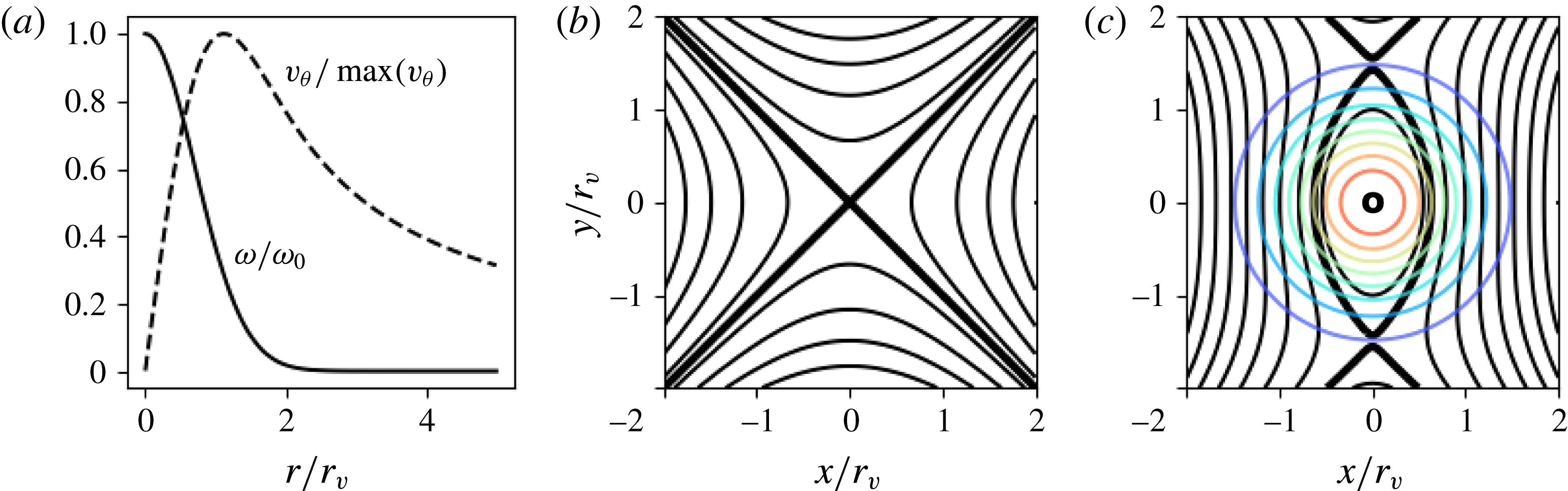
For example, consider a Gaussian initial vorticity profile (
 $\unicode[STIX]{x1D6FC}=2$
) which, for
 $\unicode[STIX]{x1D716}=0$
, produces the azimuthal flow
 $$\begin{eqnarray}\displaystyle v_{\unicode[STIX]{x1D703}}(r)=\frac{\unicode[STIX]{x1D714}_{0}r_{v}^{2}}{2r}[1-\exp [-(r/r_{v})^{2}]], & & \displaystyle\end{eqnarray}$$
shown in figure 9(a). When subjected to the simple strain flow (1.3) shown in panel (b), the instantaneous flow field at
 $t=0$
is given by the superposition of the flows due to the vortex
 $\boldsymbol{v}_{\boldsymbol{v}}$
and the external strain
 $\boldsymbol{v}_{\boldsymbol{s}}$
, as shown in panel (c) for
 $\unicode[STIX]{x1D716}/\unicode[STIX]{x1D714}_{0}\equiv \unicode[STIX]{x1D716}^{\ast }=0.2$
. This flow features critical points (Moffatt Reference Moffatt, Kambe, Nakano and Miyauchi2001) defined by
 $\boldsymbol{v}=\boldsymbol{v}_{\boldsymbol{v}}+\boldsymbol{v}_{\boldsymbol{s}}=\mathbf{0}$
, whose existence and location depend on
 $\unicode[STIX]{x1D716}^{\ast }$
. For
 $\unicode[STIX]{x1D716}^{\ast }<1/2$
, the flow contains three critical points: two saddle points along the
 $y$
-axis which define a separatrix enclosing a single centre point at the origin. Inside the separatrix, streamlines are closed and the fluid motion is vorticity dominated; outside this boundary, the streamlines are open, and the motion is strain dominated. When the separatrix intersects the vorticity profile, partial vortex destruction events are expected, where a portion of the total circulation is carried away by the external flow. As
 $\unicode[STIX]{x1D716}^{\ast }$
increases, the saddle points move toward the origin and the separatrix shrinks. At
 $\unicode[STIX]{x1D716}^{\ast }=1/2$
, the streamfunction topology changes as the two saddles annihilate the centre point. For
 $\unicode[STIX]{x1D716}^{\ast }>1/2$
there exists a single saddle point at the origin and all streamlines are open. In this case, the initial flow field predicts complete destruction of the vortex.
Initial flow geometry for a Gaussian vortex under external strain. (a) The normalized vorticity profile (solid line) and azimuthal velocity profile (dashed line); (b) the external strain flow given by (1.3), with streamlines (black), saddle point (X) and flow direction specified by arrows; and (c) the superposition of the flows in panels (a) and (b) for
 $\unicode[STIX]{x1D716}^{\ast }=0.2$
, with saddle points (X) and centre point (O), separatrix (thick black line), streamlines (black) and vorticity contours (coloured).

Further information can be obtained from the instantaneous flow field by studying spatial derivatives of the velocity field. Using this approach, Okubo and Weiss independently derived approximate short-term descriptions of the 2-D Euler equations (Okubo Reference Okubo1970; Weiss Reference Weiss1991) which have been widely studied in the context of 2-D turbulence. Following Weiss, local solutions are found to equations (1.1) for the evolution of the vorticity gradient
 $\unicode[STIX]{x1D735}\unicode[STIX]{x1D714}$
in the Lagrangian frame, under the assumption that strain and vorticity vary slowly relative to
 $\unicode[STIX]{x1D735}\unicode[STIX]{x1D714}$
. The solutions take the form
 $$\begin{eqnarray}\displaystyle \frac{\text{d}}{\text{d}t}\unicode[STIX]{x1D735}\unicode[STIX]{x1D714}\propto \exp Q^{1/2}t, & & \displaystyle\end{eqnarray}$$
where
 $Q=\unicode[STIX]{x1D713}_{xy}^{2}-\unicode[STIX]{x1D713}_{xx}\unicode[STIX]{x1D713}_{yy}$
is the Okubo–Weiss parameter, with subscripts indicating partial derivatives. Here,
 $Q$
is identified as the square of the eigenvalues of the velocity gradient tensor
 $\unicode[STIX]{x1D735}\boldsymbol{v}$
, which is equal to the difference of the squared strain magnitude and the squared vorticity,
 $Q=s^{2}-\unicode[STIX]{x1D714}^{2}$
. Normalizing to the vorticity yields
 $Q/\unicode[STIX]{x1D714}^{2}\equiv Q^{\ast }=s^{\ast 2}-1$
, so
 $Q$
is a measure of the local strain-to-vorticity ratio. Equation (3.12) admits oscillatory solutions when the vorticity dominates (
 $s^{\ast }<1$
), and exponential solutions when the strain dominates (
 $s^{\ast }>1$
). The oscillatory solutions are associated with stable vortices, and the exponential solutions are associated with filamentation behaviour (i.e. the forward enstrophy cascade). Although the assumption used to derive (3.12) was found to be valid only in certain regions of flow (Basdevant & Philipovitch Reference Basdevant and Philipovitch1994), the Okubo–Weiss result has been extended to higher orders of approximation and to three dimensions (Hua & Klein Reference Hua and Klein1998; Haller Reference Haller2005), and is widely used to differentiate stable vortex structures from regions of turbulent cascade activity.
Knowledge of the full flow field is necessary to find the streamfunction separatrix, whereas the Okubo–Weiss stability criterion can be calculated locally by differentiating the velocity field. Both criteria are valid on short time scales where the vorticity is static. On longer time scales the nonlinear evolution of the vorticity field must be taken into account, and so these stability criteria may be inaccurate. For example, the centre of a circular vortex patch with
 $0.123<\unicode[STIX]{x1D716}^{\ast }<0.5$
initially follows closed streamlines, whereas the nonlinear K81 theory predicts eventual destruction. However, both the separatrix and the Okubo–Weiss criterion are useful as approximate predictors of the local stability of the vorticity on short time scales.
4 Data
Experimental data for the evolution of an initially axisymmetric electron plasma vortex under a simple strain flow were shown in figure 1 for two values of normalized strain,
 $\unicode[STIX]{x1D716}^{\ast }=$
0.116 and 0.13, that are below and above the critical strain threshold. In this section, we compare these and other data, and corresponding vortex-in-cell simulations with theoretical predictions of the elliptical patch model. Finally, departures from the elliptical patch theory are studied using smooth profiles.
4.1 Tests of the elliptical patch model
Data are presented here from experiments with the 8ST comparing elliptical distortions of a strained vortex to predictions of the elliptical patch theory (Moore & Saffman Reference Moore, Saffman, Rogers, Olsen and Goldburg1971; Kida Reference Kida1981). Ellipses are fit to the measured half-maximum vorticity contours using the numerical routine described in § 2. This yields experimentally determined values of the aspect ratio of the ellipse
 $\unicode[STIX]{x1D706}$
and the orientation
 $\unicode[STIX]{x1D709}$
with respect to the applied strain axis, which are compared directly to the theory with no fitted parameters. For comparison to the patch model, quasi-flat initial vorticity profiles are used, where
 $\unicode[STIX]{x1D714}(r)$
is approximately given by (2.5) with smoothness exponent
 $\unicode[STIX]{x1D6FC}\geqslant 5$
.
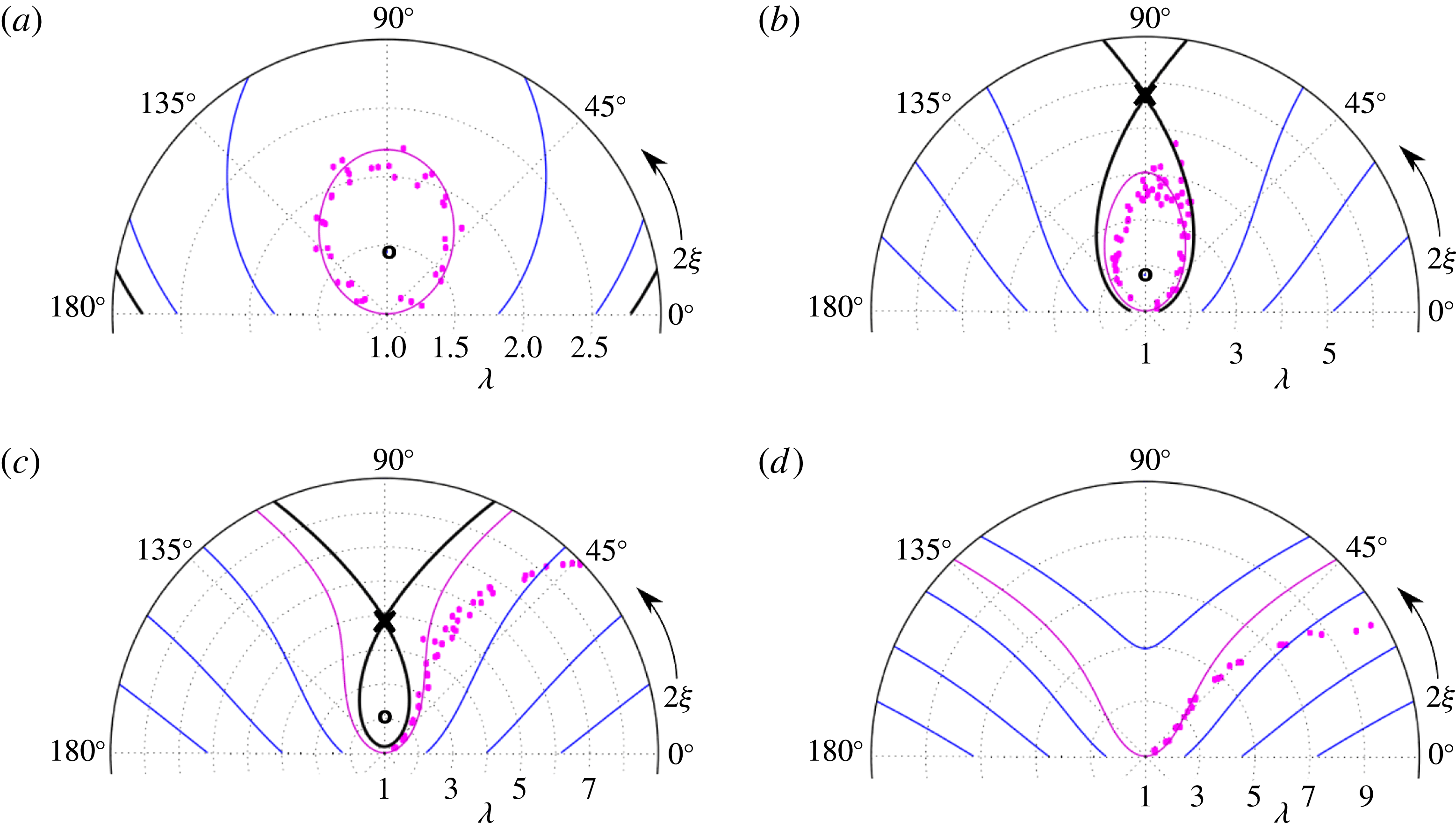
Comparison of experimental data and predictions of the K81 theory in polar
 $(\unicode[STIX]{x1D706},2\unicode[STIX]{x1D709})$
space for a quasi-flat vortex under external strain, with
 $\unicode[STIX]{x1D716}^{\ast }=$
(a) 0.087, (b) 0.116, (c) 0.13 and (d) 0.152. Contours of the K81 Hamiltonian are shown, including open orbits (blue lines), the separatrix (thick black line) and the
 $C=1$
orbit (magenta line). Fixed points of the K81 system are shown as (X) and (O), and experimental data are shown as magenta circles.

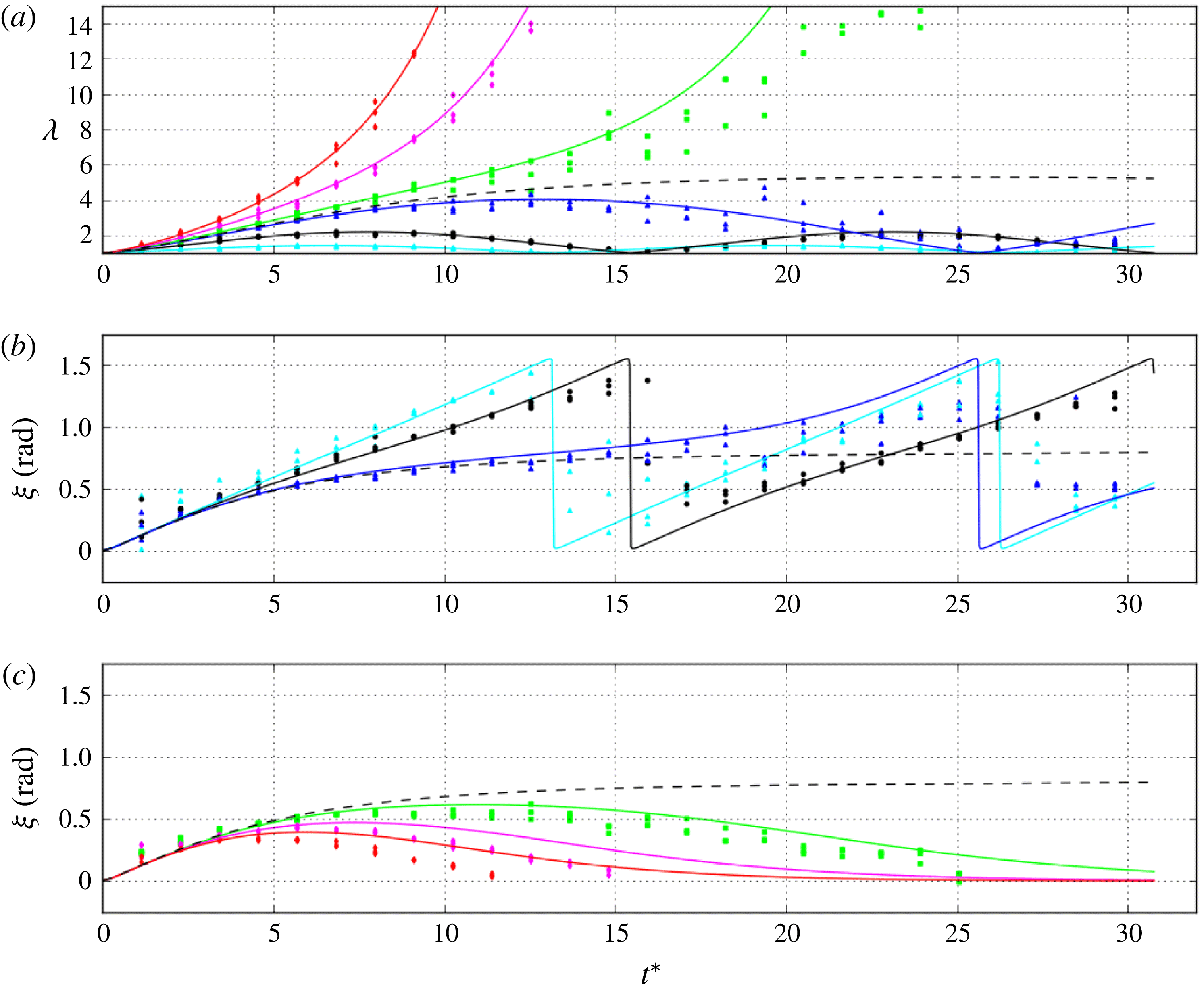
Comparison of experimental data and the K81 theory for a quasi-flat vortex with
 $C=1$
under external strain. (a)
 $\unicode[STIX]{x1D706}(t^{\ast })$
(b)
 $\unicode[STIX]{x1D709}(t^{\ast })$
(closed orbits) and (c)
 $\unicode[STIX]{x1D709}(t^{\ast })$
(open orbits) where
 $t^{\ast }=t\unicode[STIX]{x1D714}_{0}$
and
 $\unicode[STIX]{x1D714}_{0}=228~\text{krad}~\text{s}^{-1}$
, for normalized strains
 $\unicode[STIX]{x1D716}^{\ast }=0.044$
(cyan), 0.087 (black), 0.116 (blue), 0.13 (green), 0.152 (magenta) and 0.173 (red). Predictions of K81 elliptical patch theory are shown as solid lines, including the threshold orbit
 $\unicode[STIX]{x1D716}^{\ast }=0.123$
(black dashed line).

The evolution of
 $(\unicode[STIX]{x1D706},\unicode[STIX]{x1D709})$
are shown in figure 10 for an initially axisymmetric vortex with
 $\unicode[STIX]{x1D6FC}\approx 6$
(cf. figure 5
b), subject to a constant external strain flow given by (1.3). These data are compared to the K81 prediction for
 $C=1$
. Evolution of the ellipse parameters
 $(\unicode[STIX]{x1D706},2\unicode[STIX]{x1D709})$
is plotted for normalized strain
 $\unicode[STIX]{x1D716}^{\ast }=0.087$
, 0.116, 0.13 and 0.152 (panels (a)–(d), respectively), with central vorticity
 $\unicode[STIX]{x1D714}_{0}=228~\text{krad}~\text{s}^{-1}$
. Data are taken at intervals of
 $5~\unicode[STIX]{x03BC}\text{s}$
(
 $1.1\,\unicode[STIX]{x1D714}_{0}^{-1}$
), and repeated three times for statistics. Contours of the K81 Hamiltonian (3.5) are plotted over the data including open orbits, the
 $C=1$
orbit and the separatrix. Note that in figure 10(c) the circular initial condition is unstable, although closed orbits still exist inside the separatrix; whereas in panel (d) the separatrix has disappeared.
These data are also plotted versus normalized time in figure 11, with (a)
 $\unicode[STIX]{x1D706}(t^{\ast })$
and (b,c)
 $\unicode[STIX]{x1D709}(t^{\ast })$
, for six values of strain including
 $\unicode[STIX]{x1D716}^{\ast }=0.044$
, 0.087, 0.116, 0.13, 0.152 and 0.173. Predictions of the K81 theory for
 $C=1$
are shown as solid lines. The lowest strain values
 $\unicode[STIX]{x1D716}^{\ast }=0.044$
, 0.087 and 0.116 are below the dynamical stability threshold
 $\unicode[STIX]{x1D716}_{d}^{\ast }(C=1)\approx 0.123$
(shown as dashed lines), so the system executes periodic orbits in
 $(\unicode[STIX]{x1D706},\unicode[STIX]{x1D709})$
space. The highest strain values
 $\unicode[STIX]{x1D716}^{\ast }=0.13$
, 0.152 and 0.173 are above the threshold, so
 $\unicode[STIX]{x1D706}$
grows without bound as
 $\unicode[STIX]{x1D709}$
approaches 0.
The data in figures 10 and 11 generally agree with the theory, with a few notable exceptions. Since behaviour of the K81 system is unstable near the separatrix, data for the strain values just above and below the threshold (i.e.
 $\unicode[STIX]{x1D716}^{\ast }=0.116$
and 0.13) become noisy at later times. For the above threshold cases (
 $\unicode[STIX]{x1D716}^{\ast }=0.13$
, 0.152 and 0.173), the experimentally measured
 $\unicode[STIX]{x1D709}$
diverges from that of the theory when
 $\unicode[STIX]{x1D706}$
is large. This is a manifestation of the dump rotation effect discussed in § 2; since the ellipse continues to rotate slightly during the diagnosis process, the data here are corrected using a uniform shift of
 $\unicode[STIX]{x0394}\unicode[STIX]{x1D709}=-10^{\circ }$
, but the rotation shift decreases as the vortex distorts, according to (3.1).
Dynamics of unstable elliptical vortices above the critical strain threshold. (a) Data (circles) for
 $\unicode[STIX]{x1D706}(t^{\ast })$
for
 $\unicode[STIX]{x1D716}^{\ast }=0.136$
, 0.159, 0.181, 0.204, 0.227, 0.249, 0.272 (blue to red), with exponential fits (lines), where
 $\unicode[STIX]{x1D714}_{0}=195~\text{krad}~\text{s}^{-1}$
. (b) Normalized time constant of the exponential fits
 $\unicode[STIX]{x1D70F}^{\ast }\equiv \unicode[STIX]{x1D70F}\unicode[STIX]{x1D714}_{0}$
for
 $\unicode[STIX]{x1D714}_{0}=195$
(blue circles), 260 (green squares) and 326 (magenta triangles)
 $\text{krad}~\text{s}^{-1}$
. Also shown is the K81 theoretical prediction (solid black line), that assuming passive vorticity
 $\unicode[STIX]{x1D70F}^{\ast }=1/2\unicode[STIX]{x1D716}^{\ast }$
(dashed black line) and the stability boundary
 $\unicode[STIX]{x1D716}_{d}^{\ast }(C=1)\approx 0.123$
(dotted red line).

Well above the critical strain threshold
 $\unicode[STIX]{x1D716}^{\ast }\gg \unicode[STIX]{x1D716}_{c}^{\ast }$
, the K81 elliptical patch theory predicts exponential behaviour
 $\unicode[STIX]{x1D706}(t)=\exp (t/\unicode[STIX]{x1D70F})$
, where
 $\unicode[STIX]{x1D70F}=1/2\unicode[STIX]{x1D716}$
(cf. (2.6)). For
 $\unicode[STIX]{x1D716}^{\ast }>\unicode[STIX]{x1D716}_{d}^{\ast }$
, exponential curves are fit to data for
 $\unicode[STIX]{x1D706}(t)$
to find
 $\unicode[STIX]{x1D70F}$
. Figure 12(a) shows measurements of
 $\unicode[STIX]{x1D706}(t)$
for
 $\unicode[STIX]{x1D714}_{0}=195~\text{krad}~\text{s}^{-1}$
and
 $\unicode[STIX]{x1D716}^{\ast }=0.136$
, 0.159, 0.181, 0.204, 0.227, 0.249, 0.272 with exponential fits. Figure 12(b) shows the normalized time constant
 $\unicode[STIX]{x1D70F}^{\ast }\equiv \unicode[STIX]{x1D70F}\unicode[STIX]{x1D714}_{0}$
associated with the exponential fits as a function of
 $\unicode[STIX]{x1D716}^{\ast }$
for
 $\unicode[STIX]{x1D714}_{0}=195$
, 260 and
 $326~\text{krad}~\text{s}^{-1}$
, compared to the K81 prediction. The prediction assuming passive vorticity (
 $\unicode[STIX]{x1D70F}=1/2\unicode[STIX]{x1D716}$
) is shown, as is the K81 stability limit
 $\unicode[STIX]{x1D716}_{d}^{\ast }(C=1)\approx 0.123$
. Figure 12 shows that the assumption of passive vorticity is accurate for roughly
 $\unicode[STIX]{x1D716}^{\ast }>0.20$
; whereas for
 $0.123<\unicode[STIX]{x1D716}^{\ast }<0.20$
the stretching rate is reduced (i.e. the lifetime of the vortex is extended), and
 $\unicode[STIX]{x1D706}(t)$
is not exactly exponential because the system stalls near the saddle point.
Demonstration of MS71 strained vortex equilibria. Data are obtained using a slow linear ramp function
 $\unicode[STIX]{x1D716}^{\ast }\propto t$
, for
 $\unicode[STIX]{x1D714}_{0}=143~\text{krad}~\text{s}^{-1}$
(red triangles),
 $182~\text{krad}~\text{s}^{-1}$
(green squares),
 $228~\text{krad}~\text{s}^{-1}$
(magenta circles) and
 $313~\text{krad}~\text{s}^{-1}$
(blue triangles). They are compared to the stable branch (solid line) of the MS71 theory (3.8). The unstable branch is also shown (dashed line). Data and predictions for the maximum aspect ratio in a K81 orbit
 $\unicode[STIX]{x1D706}_{m}$
are shown as well, with theory given by (3.9) (dotted line) and data (black diamonds).

For the case of constant strain imposed on an initially axisymmetric vortex, as in figure 10, stationary solutions are not possible. However, if the strain is gradually increased, the system can be expected to behave adiabatically. In this case, the action
 $J$
remains approximately zero, such that the
 $(\unicode[STIX]{x1D706},\unicode[STIX]{x1D709})$
are given by the MS71 equilibrium solution (3.8). Data are shown in figure 13, where
 $\unicode[STIX]{x1D706}$
is studied by the imposition of a slow, linearly ramped strain, for
 $\unicode[STIX]{x1D714}_{0}=143$
, 182, 228 and
 $313~\text{krad}~\text{s}^{-1}$
; and ramp rates in the range
 $\text{d}\unicode[STIX]{x1D716}^{\ast }/\text{d}t^{\ast }=0.0025{-}0.005$
. The theoretical equilibria (3.8) are shown, including both the stable and unstable branches. The data agree with the theory, up to the stability limit of
 $\unicode[STIX]{x1D716}_{c}^{\ast }\approx 0.15$
to within the experimental uncertainty, implying that the system is behaving adiabatically. However, numerical solutions to (3.2) and (3.3) indicate that a small-amplitude orbit may be excited due to the kink in
 $\unicode[STIX]{x1D716}(t)$
as the linear ramp begins (Notte et al.
Reference Notte, Fajans, Chu and Wurtele1993).
Also shown in figure 13 is the maximum aspect ratio
 $\unicode[STIX]{x1D706}_{m}$
reached by a K81 orbit with
 $C=1$
(3.9), with data for
 $\unicode[STIX]{x1D716}^{\ast }=0.045$
, 0.087 and 0.116, corresponding to the orbits shown in figure 10. Again, the data and theory are in close agreement.
Shown in figure 14 are experimental measurements of both the equilibrium and dynamical stability thresholds for quasi-flat vortices with
 $\unicode[STIX]{x1D6FC}\geqslant 5$
. These data are compared to results of vortex-in-cell simulations, and predictions of the elliptical patch theory
 $\unicode[STIX]{x1D716}_{c}^{\ast }\approx 0.15$
and
 $\unicode[STIX]{x1D716}_{d}^{\ast }(C=1)\approx 0.123$
. Experimentally, the dynamical stability threshold is found by observing
 $\unicode[STIX]{x1D706}$
at late times in the evolution under constant strain (
 $t_{f}\sim 30\unicode[STIX]{x1D714}_{0}^{-1}$
, cf. figure 11). These measurements of
 $\unicode[STIX]{x1D716}_{d}^{\ast }(C=1)$
are plotted against the peak vorticity
 $\unicode[STIX]{x1D714}_{0}$
in figure 14, where the bottom (top) end of the error bar corresponds to a strain where five consecutive runs show stable (unstable) behaviour. A similar technique is used to measure the equilibrium stability limit
 $\unicode[STIX]{x1D716}_{c}^{\ast }$
. In this case, the strain is slowly increased using a linear ramp time dependence with rate
 $\text{d}\unicode[STIX]{x1D716}^{\ast }/\text{d}t^{\ast }\sim 0.005$
(cf. figure 13), and then held at a particular value of
 $\unicode[STIX]{x1D716}^{\ast }$
to determine the stability. The stability thresholds are found in a similar manner using vortex-in-cell simulations. The experimental measurements give
 $\unicode[STIX]{x1D716}_{c}^{\ast }=0.15\pm 0.01$
and
 $\unicode[STIX]{x1D716}_{d}^{\ast }(C=1)=0.124\pm 0.006$
. The simulations give
 $\unicode[STIX]{x1D716}_{c}^{\ast }=0.145{-}0.147$
and
 $\unicode[STIX]{x1D716}_{d}^{\ast }(C=1)=0.123{-}0.125$
.
Stability threshold measurements versus peak vorticity. The thresholds
 $\unicode[STIX]{x1D716}_{d}^{\ast }(C=1)$
for initially axisymmetric vortices subject to constant strain are shown (blue). Also shown are those for vortex equilibria
 $\unicode[STIX]{x1D716}_{c}^{\ast }$
using a linearly ramped strain (red). K81 and MS71 predictions are shown (
 $\unicode[STIX]{x1D716}^{\ast }=0.123$
, dashed, and 0.15, dotted), as are results of vortex-in-cell simulations (shaded). The experimental measurements are indicated by error bars (see text for details).

Thus the stability threshold observed in experiments and simulations are in good agreement with the predictions of elliptical patch theory, except for a slightly reduced value of
 $\unicode[STIX]{x1D716}_{c}^{\ast }$
in the simulations. Small deviations such as this may be associated with the smoothness of the profile at the edge of the vortex, an issue which is investigated in further detail in figure 17. Alternatively, the finite ramp time of the strain could lead to breaking of the adiabaticity and therefore slightly reduced stability limits. Constancy of the experimental results over a wide range of
 $\unicode[STIX]{x1D714}_{0}$
lends confidence that non-ideal or 3-D effects depending on the electron density are negligible.
In conclusion, many aspects of the elliptical vortex patch model studied by K81 and MS71 have been tested using realistic quasi-flat vorticity profiles that are subjected to external strain. In general, the global dynamics of the vortex cores is found to be in good agreement with the theory.
4.2 Physics beyond the elliptical patch model
The agreement between the experiments and the elliptical patch theory for quasi-flat profiles raises the following questions: How ‘flat’ must the profile be in order to agree with the theory? How is the vortex dynamics modified relative to the patch theory predictions when the profile is not sufficiently flat? These questions are addressed here by studying the full flow field as described by the 2-D Euler equations (1.1), and by studying non-flat profiles.
Evolution of a quasi-flat vortex is shown for
 $\unicode[STIX]{x1D716}^{\ast }=$
(a) 0.116 and (b) 0.13 (i.e. the same data shown in figure 1). Also shown are streamlines (black lines), the separatrix (thick black line), saddle points (X), centre points (O) and the Okubo–Weiss stability boundary defined by
 $Q=0$
(dashed line). Note the topological change of the streamfunction between fourth and fifth panels in row (b).

The vorticity evolution data shown in figure 1 for
 $\unicode[STIX]{x1D716}^{\ast }=$
0.116 and 0.13 are plotted again in figure 15, with overlaid streamlines, the separatrix and the Okubo–Weiss stability criterion
 $Q=0$
. At
 $t=0$
, a small amount of circulation exists outside the separatrix; as the vorticity evolves, the separatrix changes accordingly. Below the critical strain threshold (panel (a)), peripheral vorticity is carried into filaments exterior to the separatrix, while the majority of the circulation remains on closed streamlines inside the separatrix. Above the critical threshold (panel (b)), the separatrix shrinks as the vortex distorts. The saddle points move inward and annihilate the centre point at the origin between the fourth and fifth panels, thus changing the streamfunction topology as the vortex is destroyed. The Okubo–Weiss local stability criterion shows qualitatively similar behaviour to the separatrix, disappearing at the same point in figure 15(b). Quantitatively, however, stable regions predicted by the separatrix and the Okubo–Weiss theory show a slightly different shape and spatial extent.
Local stability inside a vortex versus time, for
 $\unicode[STIX]{x1D716}^{\ast }=0.045$
(cyan), 0.087 (black), 0.116 (blue), 0.13 (green), 0.152 (magenta) and 0.173 (red). (a) The normalized total circulation, (b) circulation inside the separatrix, (c) circulation inside the Okubo–Weiss stability boundary and (d) value of the normalized Okubo–Weiss parameter at the origin, compared to the stability threshold (dashed line). Note that
 $\unicode[STIX]{x1D6E4}_{sep},\unicode[STIX]{x1D6E4}_{Q}\rightarrow 0$
and
 $Q_{0}^{\ast }$
crossing zero indicate a change of the streamfunction topology.

The temporal evolution of the local stability properties are studied quantitatively in figure 16 for six values of
 $\unicode[STIX]{x1D716}^{\ast }$
. Shown are (a) the total normalized circulation integrated over the domain
 $\unicode[STIX]{x1D6E4}/\unicode[STIX]{x1D6E4}_{0}$
; (b) the circulation contained inside the separatrix
 $\unicode[STIX]{x1D6E4}_{sep}/\unicode[STIX]{x1D6E4}_{0}$
; (c) the circulation inside the
 $Q=0$
surface
 $\unicode[STIX]{x1D6E4}_{Q}/\unicode[STIX]{x1D6E4}_{0}$
; and (d) the normalized Okubo–Weiss parameter evaluated at the origin
 $Q_{0}^{\ast }$
, where the stability boundary
 $Q_{0}^{\ast }=0$
is shown as a black dashed line. Here,
 $\unicode[STIX]{x1D6E4}_{sep}$
and
 $\unicode[STIX]{x1D6E4}_{Q}$
are calculated as
 $\int _{S}\unicode[STIX]{x1D714}\,\text{d}A$
where
 $S$
corresponds to the region enclosed by the separatrix or the
 $Q=0$
surface. Error bars show averages over three data points. These results are calculated from the same data shown in figures 1, 10 and 11. At late times, figure 16(a) demonstrates loss of circulation to the wall gaps (note that for the three strain values above the threshold,
 $\unicode[STIX]{x1D6E4}/\unicode[STIX]{x1D6E4}_{0}$
eventually tends to zero). Panels (b) and (c) show the shrinking and disappearance of the separatrix and Okubo–Weiss stable region for the cases above the strain threshold, and destabilization of peripheral circulation for the case slightly below threshold. In figure 16(d),
 $Q_{0}^{\ast }=s^{\ast 2}-1$
increases dramatically from its initial value
 $4\unicode[STIX]{x1D716}^{\ast 2}-1$
due to the self-strain
 $s_{v}$
as the vortex distorts. For the three strains above the threshold,
 $Q_{0}^{\ast }$
crosses the stability boundary as the stream function changes topology. Thus, the initial streamfunction separatrix and the Okubo–Weiss criteria fail to predict the eventual destruction of the vortex due to nonlinear evolution of the vorticity. The temporal behaviour of
 $\unicode[STIX]{x1D6E4}_{sep}$
and
 $\unicode[STIX]{x1D6E4}_{Q}$
are comparable, although not exactly in agreement. Further study of these local stability criteria is left for future work.
Hurst et al. (Reference Hurst, Danielson, Dubin and Surko2016) demonstrated a slightly reduced critical strain threshold for smooth, Gaussian vorticity profiles relative to quasi-flat ones. This effect is analysed further in figure 17, which shows the dynamical threshold
 $\unicode[STIX]{x1D716}_{d}^{\ast }(C=1)$
versus the smoothness exponent
 $\unicode[STIX]{x1D6FC}$
. Experimental and numerical data are shown, as is the K81 strain threshold
 $\unicode[STIX]{x1D716}_{d}^{\ast }(C=1)\approx 0.123$
. The error bars are found in the same manner described above in the discussion of figure 14. Here, the simulations use profiles given by (2.5), with
 $\unicode[STIX]{x1D6FC}$
varying from 2 to 10. For the experimental data,
 $\unicode[STIX]{x1D6FC}$
is found using a fit to (2.5). Both the experimental and numerical data show a clear shift to lower stability threshold at low
 $\unicode[STIX]{x1D6FC}$
(i.e. approaching Gaussian profiles). Data are taken here for
 $\unicode[STIX]{x1D714}_{0}=347{-}571~\text{krad}~\text{s}^{-1}$
, and radius
 $r_{v}=0.1{-}0.2~r_{w}$
. The experimental profiles agree closely with (2.5). Other data (not shown here) suggest that the threshold is lowered by approximately 10 % for
 $r_{v}\approx 0.3r_{w}$
, likely due to influence from the wall. Additionally, results for profiles which are not good fits to (2.5) show that the threshold can be sensitive to specific details of the profile.
Data for the evolution of a Gaussian vortex relative to a quasi-flat vortex is shown in figure 18. Here, panel (a) shows a Gaussian vortex with
 $\unicode[STIX]{x1D6FC}\approx 2$
, and panel (b) shows a quasi-flat vortex with
 $\unicode[STIX]{x1D6FC}\approx 8$
. For both profiles,
 $\unicode[STIX]{x1D714}_{0}=785~\text{krad}~\text{s}^{-1}$
and
 $\unicode[STIX]{x1D716}^{\ast }=0.112$
. The strain magnitude is chosen just slightly below the K81 threshold, such that the flat vortex survives, but the Gaussian vortex is destroyed, demonstrating the threshold shift shown in figure 17. A plausible explanation for this shift is that the smooth profiles feature substantial filamentary structures near the saddle points which augment the total strain in the vortex core. In contrast, although quasi-flat profiles may also show filamentary behaviour, the circulation contained in these filaments is small and therefore the effect of the filaments on the core is negligible.
Dynamical stability threshold for constant strain
 $\unicode[STIX]{x1D716}_{d}^{\ast }(C=1)$
versus smoothness exponent
 $\unicode[STIX]{x1D6FC}$
, where
 $\unicode[STIX]{x1D6FC}=2$
corresponds to a Gaussian profile and
 $\unicode[STIX]{x1D6FC}\rightarrow \infty$
to a patch profile. Shown are the K81 theoretical stability limit (dashed line), simulations (black error bars, shaded) and experimental data (magenta error bars).

Experimental evolution of vorticity (colour maps) and streamfunction (lines) for (a) a Gaussian profile, and (b) a quasi-flat profile with
 $\unicode[STIX]{x1D6FC}\approx 8$
. Both rows (a) and (b) correspond to
 $\unicode[STIX]{x1D714}_{0}=785~\text{krad}~\text{s}^{-1}$
,
 $\unicode[STIX]{x1D716}^{\ast }=0.112$
and panels are separated by time
 $t^{\ast }=12.56$
beginning with
 $t^{\ast }=0$
.

For a smooth vortex below the critical destruction threshold, although the core may survive, the outer circulation can be stripped away to some degree. Figure 19 shows the total remaining circulation in a vortex subjected to constant strain for time
 $t_{f}=25\unicode[STIX]{x1D714}_{0}^{-1}$
. The experimental data agree well with simulations for both a quasi-flat profile with
 $\unicode[STIX]{x1D6FC}\approx 7$
and a smooth profile with
 $\unicode[STIX]{x1D6FC}=2$
. The K81 destruction threshold is shown as well. The data show that smooth vortices suffer heavy stripping due to the external strain, even well below the destruction threshold.
Fraction of the circulation remaining in a vortex after a straining event. Shown are experimental data (magenta) for a quasi-flat vortex with
 $\unicode[STIX]{x1D6FC}\approx 7$
(diamonds) and a Gaussian vortex with
 $\unicode[STIX]{x1D6FC}\approx 2$
(squares), and simulation data (black, with lines) for
 $\unicode[STIX]{x1D6FC}=7$
(triangles) and
 $\unicode[STIX]{x1D6FC}=2$
(circles). The K81 stability threshold is indicated by the dashed line.

The K81 elliptical patch model preserves energy, and therefore trajectories in phase space are given by contours of the Hamiltonian (3.5). However, it is observed that these orbits can undergo inviscid damping (i.e. spatial Landau damping (Schecter et al.
Reference Schecter, Dubin, Cass, Driscoll, Lansky and O’Neil2000; Balmforth et al.
Reference Balmforth, Smith and Young2001; Turner et al.
Reference Turner, Gilbert and Bassom2008)) when the vorticity profile is sufficiently non-flat. This effect is demonstrated in figure 20 using an initial profile which has a flat core (
 $\unicode[STIX]{x1D6FC}\approx 8$
) and a low-vorticity tail exterior to the core (cf. figure 5
c). Figure 20(a–c) shows evolution of the ellipse parameters
 $(\unicode[STIX]{x1D706},2\unicode[STIX]{x1D709})$
in response to constant strain of magnitude
 $\unicode[STIX]{x1D716}^{\ast }=0.045$
, 0.09 and 0.108, respectively. Shown here are experimental data and simulation data, where the simulations use an initial vorticity profile identical to the experimental one. The data are compared to the
 $C=1$
contour of the K81 Hamiltonian. The energy
 $H$
is calculated from
 $(\unicode[STIX]{x1D706},\unicode[STIX]{x1D709})$
, and plotted versus time in figure 20(d–f) for experimental and numerical data, corresponding to the damped orbits in panels (a–c). The amount of remaining circulation at the end of each data set is
 $\unicode[STIX]{x1D6E4}_{f}/\unicode[STIX]{x1D6E4}_{0}\approx$
1 (panel a), 0.95 (panel b) and 0.9 (panel c). The evolution of the vorticity and streamfunction is shown for two damped orbits in figure 21 with
 $\unicode[STIX]{x1D716}^{\ast }=$
(a) 0.045 and (b) 0.09 (corresponding to the data in figure 20(a,b)). Both cases clearly show filamentation behaviour, and panel (b) also shows circulation loss to the wall.
Inviscid damping of K81 orbits in
 $(\unicode[STIX]{x1D706},2\unicode[STIX]{x1D709})$
space. (a–c) Experimental data (magenta circles) and simulation results (black triangles), as well as contours of
 $H$
for the
 $C=1$
orbit (magenta line) and separatrix (black line), and the stable equilibrium point (green square), for
 $\unicode[STIX]{x1D716}^{\ast }=$
(a) 0.045, (b) 0.09 and (c) 0.108. (d–f) The temporal evolution of
 $H$
corresponding to the data in (a–c), relative to the initial value (dashed) and the value at the stable equilibrium (dotted).

Vorticity (colour maps) and streamfunction (lines) evolution during inviscid damping of a K81 orbit, for
 $\unicode[STIX]{x1D716}^{\ast }=$
(a) 0.045 and (b) 0.09. Here,
 $\unicode[STIX]{x1D714}_{0}=458~\text{krad}~\text{s}^{-1}$
, and data are shown at time intervals
 $\unicode[STIX]{x0394}t^{\ast }=9.16$
beginning with
 $t^{\ast }=0.916$
.

Here, the energy
 $H$
(3.5) associated with the
 $m=2$
elliptical distortions decreases as energy is transferred to other wavenumbers, either by differential rotation or filamentation. Thus, the
 $C=1$
orbit evolves toward the local minimum of
 $H$
at the stable centre point given by the lower branch of (3.8). In figure 20(a,b), the damping drives the system very close to the equilibrium. However in panel (c), the damping saturates at a finite orbit amplitude. In this case, the tail is stripped away suddenly and the damping shuts off, and the remaining flat core executes a nutation mode. Both the experiments and simulations show similar behaviour, although the onset and rate of damping is slightly different.
Based on these observations, inviscid Landau damping of an elliptical vortex in the presence of external strain differs qualitatively from the freely relaxing case studied previously (Schecter et al. Reference Schecter, Dubin, Cass, Driscoll, Lansky and O’Neil2000; Balmforth et al. Reference Balmforth, Smith and Young2001; Turner et al. Reference Turner, Gilbert and Bassom2008) in two major ways. First, rather than damping toward axisymmetry, the system damps toward a steady elliptical state similar to the stable equilibria given by MS71. In the case of zero strain, the damping may saturate as a rotation mode, whereas with non-zero strain the saturated state can be a nutation mode. Secondly, circulation may be stripped and lost to the wall due to the external strain. Thus, in addition to damping via differential rotation and filamentation, damping may occur through an ‘evaporative’ process associated with circulation crossing the separatrix. Note that in figure 20 panels (b) and (c) evidence of circulation loss implies that the evaporative damping mechanism is active, whereas in panel (a) no circulation loss is observed. Here, inviscid damping of the K81 orbit is demonstrated for a profile which is quasi-flat in the core, but with a tail of circulation at the edge of the vortex, as shown in figure 5(c). Other various data from the 8ST (not shown here) indicate that damping may occur for a broad range of non-flat profiles.
5 Summary and discussion
This work focuses on the behaviour of a 2-D ideal vortex structure under the influence of external strain. The experiments are done in an electron plasma confinement apparatus which was designed specifically to study vortex dynamics under the influence of an external flow. Corresponding simulations are conducted using the vortex-in-cell technique. External strain is imposed by adjusting the boundary conditions in two dimensions. Details of the experimental technique are given, including a discussion of the analogy between a 2-D ideal fluid and pure electron plasma. Quasi-flat initial vorticity profiles are prepared, and the resulting dynamics is compared to a simple model which treats the vorticity distribution as piecewise constant in an elliptical region.
The theoretical predictions of K81 (Kida Reference Kida1981) are confirmed, that strained vortices execute closed orbits below a certain strain threshold, where the aspect ratio and orientation of the ellipse oscillate periodically. Above this threshold, the experiments confirm that the aspect ratio increases without bound in response to the external strain and the entire vortex is destroyed. Measurements of the critical strain threshold are in good agreement with results of simulations and theoretical predictions. Additionally, when the strain is slowly ramped up, the experimental data agree with the stable elliptical patch equilibria given by Moore & Saffman (Reference Moore, Saffman, Rogers, Olsen and Goldburg1971). The elliptical patch variables
 $(\unicode[STIX]{x1D706},\unicode[STIX]{x1D709})$
are measured directly by diagnosing the vorticity field, and the observed dynamics agrees quantitatively with the theoretical predictions.
When the initial vorticity profile is relatively smooth, the dynamics of strained vortices diverges from the predictions of the elliptical patch model. Here, stability of the vorticity is a local matter, so vortices may experience partial or total destruction. During total destruction, saddle points move smoothly into the profile, eventually causing a topological change in the fluid streamfunction as the strain overcomes rotation at the centre of the vortex. Linear predictions from the initial flow field and the Okubo–Weiss criterion fail to predict the eventual destruction of vortices in the range
 $\unicode[STIX]{x1D716}_{d}^{\ast }<\unicode[STIX]{x1D716}^{\ast }<1/2$
due to additional strain associated with the vortex distortion. Experiments show that smooth profiles exhibit slightly reduced stability limits relative to quasi-flat profiles, possibly due to additional self-strain produced by filaments which form near the saddle points. Finally, non-flat profiles are found to execute periodic orbits similar to those discussed in K81, but the orbits may experience inviscid damping, reminiscent of the work of Schecter et al. (Reference Schecter, Dubin, Cass, Driscoll, Lansky and O’Neil2000), Balmforth et al. (Reference Balmforth, Smith and Young2001) and Turner et al. (Reference Turner, Gilbert and Bassom2008). This is manifested by a decrease in the orbit amplitude, where the system evolves toward the stable equilibria given by MS71 and may saturate as a K81 nutation mode. In general, it is observed that the dynamics of a vortex core can be modified due to the behaviour of peripheral circulation near the vortex edge, leading to deviations from the elliptical patch theory.
These results are relevant to a variety of quasi-2-D fluid systems found in man-made and natural environments. Examples include geophysical fluids, strongly magnetized plasmas, astrophysical disks and various engineering and industrial applications. A common theme in many of these systems is that the transport of heat, momentum and particulate matter (i.e. passive tracers, chemicals, etc.) is often dominated by the formation and persistence of coherent vortices. For example, vortices appear routinely in the Earth’s atmosphere and oceans, and they have a substantial impact on weather and climate behaviour (Dritschel & Legras Reference Dritschel and Legras1993). In strongly magnetized toroidal laboratory plasmas, quasi-2-D turbulent transport has challenged attempts to generate the conditions necessary for nuclear fusion, although recent work has shown that transport can be suppressed through an eddy decorrelation mechanism similar to the K81 destruction modes (Terry Reference Terry2000). Although many practical fluid systems feature non-2-D and non-ideal effects at some level, the 2-D ideal vortices discussed here provide a simple qualitative description of the physics involved (Tabeling Reference Tabeling2002).
Recent experimental results from the 8ST suggest opportunities for further investigations. For example, more detailed studies could be carried out regarding inviscid damping of the K81 orbits for non-flat profiles. Additionally, further studies of the Okubo–Weiss local stability criterion and its variants would be interesting. The time dependence of the external strain can be chosen arbitrarily, while this work focused only on constant or ramped strain. Further investigation of vortex adiabaticity under ramped strain would be an important direction of research. Other possibilities include a Gaussian strain pulse, which could mimic a smooth transient straining event, or a sinusoidal time dependence to produce a periodic straining scenario. Another interesting direction would be the intentional introduction of various non-2-D or non-ideal effects, with the goal of more accurately simulating flows of interest to geophysics, astrophysics and plasma physics.
Acknowledgements
We wish to acknowledge helpful conversations with W. R. Young and the expert technical assistance of the late G. Jerzewski. This work is supported by plasma partnership grants NSF no. PHY-1414570, DOE no. DE-SC0002451, and DOE no. DE-SC0016532.