I. INTRODUCTION
When the spacing between neighboring interfaces is refined down to the nanoscale regime, interface densities increase and interface dynamics dominates. Consequently, interfaces play a critical role in the response of an interface-dense material when exposed to extreme environments such as radiation, elevated temperatures and high strain and strain rates.Reference Beyerlein, Mara, Wang, Carpenter, Zheng, Han, Zhang, Kang, Nizolek and Pollock1–Reference Wang and Misra4 Recent atomic scale studies have shown that the behavior of an interface in response to forces or to extrinsic defects is strongly connected to characteristics of their interfacial dislocation network.Reference Wang and Misra4–Reference Hirth, Pond, Hoagland, Liu and Wang6 The directions of the Burgers vectors of the interfacial dislocations affect its response to an applied interfacial shear stress, determining whether it slidesReference Wang, Hoagland, Liu and Misra7, Reference Wang, Hoagland, Hirth and Misra8 or it emits dislocations.Reference Wang, Kang, Zhang, Zheng, Beyerlein and Mara5, Reference Wang, Misra and Hirth9, Reference Zhang, Wang, Beyerlein, Misra and Germann10 Such differences have also been found to influence the propensity for deformation twinningReference Zheng, Beyerlein, Wang, Carpenter, Han and Mara11, Reference Han, Carpenter, Wang, Beyerlein and Mara12 and resistance to shock compression.Reference Zhang, Germann, Wang, Liu and Beyerlein13 Regarding radiation resistance, the vacancy sink strength has been connected to the number of intersections between distinct interfacial dislocation arraysReference Demkowicz, Wang, Hoagland and Hirth2, Reference Hirth, Pond, Hoagland, Liu and Wang6 and the core of the nonplanar component of the Burgers vector.Reference Kang, Wang, Zheng and Beyerlein14 Last, the mechanism by which glide dislocations nucleate from the interface depends on the Burgers vectors of the interfacial network,Reference Wang, Kang, Zhang, Zheng, Beyerlein and Mara5, Reference Zhang, Wang, Beyerlein, Misra and Germann10, Reference Zhang, Wang, Beyerlein and Germann15 being easier for those with nonplanar Burgers vectors than with only planar Burgers vectors. These examples are just the beginning and motivate detailed analysis of interface defect structure, as well as further exploration of its effect on interface dynamics.
When two crystals are joined to form an interface, in general, there exist some overlapping regions and/or gaps at the interface due to the incompatibilities and/or the dissimilarities between the two lattices. Accompanying the removal of incompatibilities and/or the dissimilarities, interfacial dislocations (IDs) are required in forming the semicoherent interface, which act as stress annihilators to free the stresses far from the interfaces. FrankReference Frank16 and BilbyReference Bilby17 provided a theory in which the net Burgers vector content  $\vec B\left( {\vec p} \right)$ of the stress generators crossing a probe vector
 $\vec p$ lying in the interface could be determined. Driven to minimize chemical potential energy of interfaces, atoms within the interface in the two crystals tend to match each other, forming a coherent lattice within the interface. As a consequence, the continuous distribution of interface Burgers content
 $\vec B\left( {\vec p} \right)$ will be energetically unfavorable, instead of forming discrete interface dislocations. Consequently, the open issue is how to determine the number of interface dislocations and their characters such as line sense, Burgers vector and spacing.
The O-lattice theory,Reference Bollmann18 which may be regarded as a quantized form of the Frank-Bilby (F-B) theory, was developed to deal with the Burgers vectors content  $\vec B\left( {\vec p} \right)$ in a discrete fashion rather than continuous distribution.Reference Bollmann19–Reference Sutton and Balluffi24 The principle is based on the concept of “well matching”, that is optimal structures are produced in interfaces in regions centered on points where the two lattices adjoining the interface are “well matched”.Reference Sutton and Balluffi24 More precisely, if for any cell of one lattice the internal coordinates of a point, expressed as fractions of the cells edges, are identical with the fractional coordinates of the same point measured relative to a cell of the other lattice, the point is a point of “lattice matching” and it is called an O-lattice.Reference Sutton and Balluffi24 The set of all O-points constitutes the O-lattice that may be a point, line or planar lattice. Following Christian's description,Reference Nakanishi25 the different O-elements (points, lines, and planes) are separated by Wigner-Seitz cell walls.Reference Gleiter26 On constructing the interface by sectioning the O-lattice, the intersections of the Wigner-Seitz cell walls are identified with line discontinuities within the interface that are called “mathematical dislocations.” There have been numerous applications of the O-Lattice theory to interpreting observed line defect contrast at grain boundaries and interphase boundaries in the electron microscope.Reference Goodhew, Darby and Balluffi27–Reference Goodhew30 However, the O-lattice construction is purely geometrical in nature; it may or may not predict the correct interface dislocations,Reference Hirth, Pond, Hoagland, Liu and Wang6, Reference Sutton and Balluffi24 because the actual dislocation structure is dictated by minimization of the boundary energy.
It has been recognized that both theories (F-B and O-Lattice) have one major weak point corresponding to the physical assumption that determines the choice of the reference lattice. Moreover, even if the reference lattice can be reasonably chosen, several sets of interface dislocations can be predicted using the F-B theory and O-lattice theory.Reference Hirth, Pond, Hoagland, Liu and Wang6, Reference Sutton and Balluffi24 The predicted dislocation patterns and their characters may or may not be identical with experimental observation although there have been many successful examples. In a brief summary, the key issues corresponding to the two theories are (i) how to define the reference lattice and (ii) how to determine the characteristics of interface dislocations, such as the number, line sense, Burgers vector, and spacing.
Atomistic simulations with reliable empirical potentials offer a powerful capability of characterizing atomic structures of an interface. For a relaxed interface, the disregistry analysis and/or the relative displacement analysis of the relaxed structure with respect to the unrelaxed structure can provide insights in understanding the relaxation processes.Reference Kang, Wang, Zheng and Beyerlein14, Reference Kang, Wang and Beyerlein31, Reference Demkowicz, Hoagland and Hirth32 Consequently, the coherent regions presented within the interface can be identified from the relaxed interface. Thus, the regions separating the coherent regions correspond to the locations of interface defects, in other words, interface dislocation lines including the line sense and the spacing can be determined from atomistic simulations.Reference Kang, Wang and Beyerlein31, Reference Demkowicz, Hoagland and Hirth32 It is worth mentioning that atomistic simulations may or may not provide the quantitative details of the interface defects in terms of Burgers vectors except for a simple pattern of interface dislocations, because the core relaxation and the local reactions between interface dislocations often disturb the quantitative analysis.Reference Wang, Hoagland, Hirth and Misra8, Reference Demkowicz, Hoagland and Hirth32
To overcome the shortcomings in these methods, we proposed atomically informed F-B theory (AIFB) by combining the classical F-B theory and atomistic simulations. We show that the Burgers vectors for an atomically flat interface (no rotation) can be well defined in a CDP/RCDP lattice, which corresponds to the reference lattice. These Burgers vectors always differ, sometimes only slightly, from the Burgers vectors of either crystal adjoining the interface in its perfect state. In addition, the CDP/RCDP (lattice) is not simply a geometric average of the two lattices in terms of the mismatch strains and the relative twist between the two lattices.Accordingly, this article is organized as follows. In Sec. II, we briefly review the classic F-B theory, describe the atomistic simulation regarding the relaxation and defect characterization of interfaces, and finally discuss the AIFB including the procedure of determining the reference lattice and solving the atomically informed F-B equations for the interface dislocations including the Burgers vector, the line sense, and the spacing. In Sec. III, we have applied the AIFB theory to two types of interfaces, one only contains the misfit and the other contains both the misfit and the twist, to determine interface dislocations. The nonequal geometry partition of both the twist and the misfit into the two lattices has been examined. Finally, we draw the conclusions in Sec. IV.
II. ATOMICALLY INFORMED FRANK-BILBY THEORY
A. The classical Frank-Bilby theory
Frank-Bilby theory provides a way to determine the Burgers vector content  $\vec B\left( {\vec p} \right)$ of an equilibrium interface in a bicrystal. As with most treatments of the problem, all of the detailed solutions are for the homogeneous, isotropic elastic approximation of coherency and defect fields. Considering an interface between bicrystals with lattices A and B, these lattices can be related to a common median lattice (in other words, a reference lattice) by homogeneous distortion transformation matrices S A and S B. For an atomic flat interface, the distortion transformation is represented by 2 × 2 matrices and transforms the vectors in the lattices A and B to the reference lattice. Let
 $\vec p$ be a large vector (probe vector) in the interface where the vector must be large compared with any substructure within the interface, the net Burgers vector
 $\vec B( {\mathord{\buildrel{\lower3pt\hbox{$\scriptscriptstyle\rightharpoonup$}}\over p} } )$ crossing the interfacial vector
 $\vec p$ can be calculated as
 $$\vec B\left( {\vec p} \right) = \left( {S_B^{ - 1} - S_A^{ - 1} } \right)\vec p\quad,$$
where S A−1 and S B−1 are the inverse matrices of S A and S B. It is clear that the interface Burgers content  $\vec B( {\mathord{\buildrel{\lower3pt\hbox{$\scriptscriptstyle\rightharpoonup$}}\over p} } )$ is dependent on the choice of the reference lattice, which is the key source of ambiguity in the dislocation description of an interface.Reference Hirth, Pond, Hoagland, Liu and Wang6, Reference Sutton and Balluffi24 Following Knowles’ suggestionReference Knowles33 that the discrete Burgers vectors of interface dislocations are the lattice vectors in the reference lattice,
 $\vec B( {\mathord{\buildrel{\lower3pt\hbox{$\scriptscriptstyle\rightharpoonup$}}\over p} } )$ is thus expressed in the reference lattice as follows.
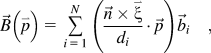 $$\vec B\left( {\mathord{\buildrel{\lower3pt\hbox{$\scriptscriptstyle\rightharpoonup$}}\over p} } \right) = \mathop\sum\limits_{i = 1}^N {\left( {{{\vec n \times \mathord{\buildrel{\lower3pt\hbox{$\scriptscriptstyle\rightharpoonup$}}\over \xi } } \over {d_i }} \cdot \vec p} \right)} \vec b_i\quad,$$
where the sum is taken over the N sets of discrete interface dislocations that are assumed to exist in the interface, b i is the Burgers vector of interface dislocation,  $\vec n$ is the normal of the interface plane,
 $\vec \xi _i$ and d i are the line sense and the spacing of the interface dislocation with the Burgers vector b i, respectively.
It has been pointed out that there are more than one set of solutions using the F-B equation,Reference Hirth, Pond, Hoagland, Liu and Wang6, Reference Sutton and Balluffi24 in other words, the F-B equation serves as the cornerstone of many attempts to account for the line defects. However, all dislocations of a particular interface are descriptions of a unique physical object with a particular atomic structure and energy. Thus, experimental observations using the electron microscopy and/or atomistic simulations are required to confirm the prediction of the F-B theory.Reference Kang, Wang, Zheng and Beyerlein14, Reference Kang, Wang and Beyerlein31–Reference Sauvage, Renaud, Deconihout, Blavette, Ping and Hono34
B. Atomistic simulations
Besides the electron microscopy, atomistic simulations can also provide the details of atomic structures of an interface, which can serve as the evidence in determining the physical solution obtained from the F-B theory. Atomistic simulations include two stages, (i) interface relaxation and (ii) defect characterization.
1. Interface relaxation
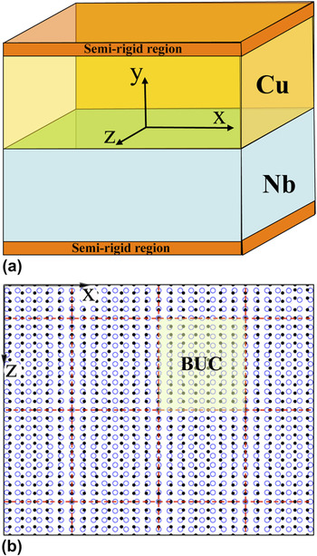
The relaxed, equilibrium interface structures are obtained by atomistic simulations with the reliable empirical interatomic potentials. The geometry of the bicrystal simulation model is shown in Fig. 1(a). The interface plane corresponds to the x-z plane. Periodic boundary conditions are applied in both the x- and z-directions and a semirigid boundary is applied in the y-direction for mimicking the response of the bulk material. In all simulations, the y dimension is sufficiently large (>10 nm) for each crystal, which is greater than the regions affected by the interfaces.Reference Kang, Wang and Beyerlein31, Reference Demkowicz, Hoagland and Hirth32
(a) The geometry of the bicrystal simulation model and (b) the natural dichromatic pattern (NDP) of the interface.

The periodic in-plane x and z dimensions, however, must be determined with respect to the orientation relationship (i.e., macroscopic degrees of freedom in defining an interface) due to the incommensurate nature of two lattices. For example, Fig. 1(b) shows the natural dichromatic pattern (NDP) of the interface. The dimensions can be chosen from the NDP corresponding to the variation of misfit strains. In general, it is hard to find the finite dimensions that are identical in both crystals. Thus by applying the additional strains to both crystals, a super boundary unit cell (BUC) can be defined, referred to as the strained-NDP. The optimal strained-NDP can be determined as follows. For example, let N xA and N xB be the total number of periodicity lying along the periodic cell dimension along the x-direction in the unrelaxed A and B crystals, respectively. Accordingly,  $X_A = N_x^{\rm{A}} \mathord{\buildrel{\lower3pt\hbox{$\scriptscriptstyle\rightharpoonup$}}\over e} _x{\mathord{\buildrel{\lower-1.6pt\hbox{$\scriptstyle \kern-3ptA$}}}} $ and
 $X_B = N_x^B \mathord{\buildrel{\lower3pt\hbox{$\scriptscriptstyle\rightharpoonup$}}\over e} _x{\mathord{\buildrel{\lower-1.6pt\hbox{$\scriptstyle \kern-3ptB$}}}} $ are the dimensions of both crystals along the x-axis. Employing the same method,
 $Z_A = N_z^A \mathord{\buildrel{\lower3pt\hbox{$\scriptscriptstyle\rightharpoonup$}}\over e} _z{\mathord{\buildrel{\lower-1.6pt\hbox{$\scriptstyle \kern-3ptA$}}}} $ and
 $Z_B = N_z^B \mathord{\buildrel{\lower3pt\hbox{$\scriptscriptstyle\rightharpoonup$}}\over e} _z{\mathord{\buildrel{\lower-1.6pt\hbox{$\scriptstyle \kern-3ptB$}}}} $ are the dimensions of both crystals along the z-axis, where
 $\mathord{\buildrel{\lower3pt\hbox{$\scriptscriptstyle\rightharpoonup$}}\over e} _i{\mathord{\buildrel{\lower-3pt\hbox{$\scriptstyle \kern-2ptA$}}}} $ is the periodicity vector of the lattice A along the i-axis. The misfit strains are
 $$\varepsilon _{xx}^{{\rm{misfit}}} \,\equiv {{2\left| {\left| {X_A } \right| - \left| {X_B } \right|} \right|} \over {\left| {X_A } \right| + \left| {X_B } \right|}}\quad {\rm{and}}\quad \varepsilon _{zz}^{{\rm{misfit}}} \,\equiv {{2\left| {\left| {Z_A } \right| - \left| {Z_B } \right|} \right|} \over {\left| {Z_A } \right| + \left| {Z_B } \right|}}\quad,$$
which varies with the choice of (N xA, N xB) and (N zA and N zB). For a chosen set of (N xA, N xB) and (N zA and N zB), the imposed strains to the ideal crystals,  $\varepsilon _{ii}^A$ and
 $\varepsilon _{ii}^B$, can be solved according the elastic theory while satisfying the equilibrium conditions,
 $\sigma _{xx}^A h_A + \sigma _{xx}^B h_B = 0$,
 $\sigma _{zz}^A h_A + \sigma _{zz}^B h_B = 0$,
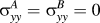 $\sigma _{yy}^A = \sigma _{yy}^B = 0$ under the periodic boundary conditions in the both x- and z-axis, where h A and h B are the thickness of the crystal in the y-direction. By applying the imposed strains
 $\varepsilon _{ii}^A$ and
 $\varepsilon _{ii}^B$ for the both crystals, a strained-NDP is created.
The bicrystal simulation model is then relaxed at zero temperature by quenching molecular dynamics with the embedded atom method (EAM) potentials.Reference Wang, Hoagland, Hirth and Misra35–Reference Demkowicz and Hoagland38 During relaxation, the two crystals are allowed to translate in the three orthogonal x-y-z directions, but restricted from rotating about the interface normal. The net forces, acting parallel and perpendicular to the interface, drive the translations. Consequently, relaxation removes these forces as well as forces on each of the atoms within the computational cell.
2. Characterization methods of interface dislocations
To determine the interface dislocations, we first construct a trial reference lattice. Useful reference structures are often interfaces in which one or two directions are nearly commensurate in both crystal lattices enabling near-coincidence site lattices (CSLs) to be generated. With a trial reference lattice, the disregistry analysis is performed to characterize interface defects. In the disregistry analysis, pairs of atoms that straddle the desired interface plane are first identified in the unrelaxed interface. Three sets of vectors with respect to three structures are calculated with the following identified pairs:  $r_{ij}^{CDP}$ describes the relative displacements of the i∼j pair in the reference lattice,
 $r_{ij}^{UnR}$ describes the relative displacements of the i∼j pair in the unrelaxed interface, and
 $r_{ij}^{Rlx}$ describes the relative displacements of the i∼j pair in the relaxed, equilibrium interface.
The vector  $r_{ij}^{U - C} = r_{ij}^{UnR} - r_{ij}^{CDP}$ describes the relative displacements corresponding to the distortion from a NDP to a CDP. Along a given probe vector, it will define the uniformly continuous distribution of interface Burgers vectors. The vector
 $r_{ij}^{R - C} = r_{ij}^{Rlx} - r_{ij}^{CDP}$ describes the relative displacements corresponding to the distortion from the relaxed interface to a CDP. Along a given probe vector, it will define the nonuniformly continuous distribution of interface Burgers vectors along the probe vector. The net vector along the probe vector is equal to the interface Burgers vectors as defined with
 $r_{ij}^{U - C}$. The vector
 $r_{ij}^{R - U} = r_{ij}^{Rlx} - r_{ij}^{UnR}$ describes the relative displacements corresponding to the distortion from the relaxed interface to a NDP. It defines the nonuniform relaxation displacement due to the formation of discrete interface dislocations. Within a periodic length of the BUC, the net vector
 $r_{ij}^{R - U} = r_{ij}^{Rlx} - r_{ij}^{UnR}$ along the probe vector is zero. According to the feature of the displacement field in association with an isolated dislocation, the displacements in the left and the right of the dislocation line have the opposite sign. Thus, the two vector fields
 $r_{ij}^{R - C}$ and
 $r_{ij}^{R - U}$ along the probe vector will provide the necessary details in determining the position of discrete interface dislocations in a real bicrystal interface. Correspondingly, the dislocation lines and their spacing can be well determined from atomistic simulations through the disregistry analysis.
C. Procedure of determining interface dislocations in AIFB
AIFB is developed by combining the F-B theory and the atomic structures of interfaces obtained by atomistic simulations to overcome the shortcomings in choosing the reference lattice in the F-B theory and in determining the Burgers vectors of interface dislocations.
Regarding a trial reference lattice, as discussed in. Sec. II. B, the possible Burgers vectors can be defined in the reference lattice. Disregistry analysis is performed for the relaxed, equilibrium interface. Following the procedure described in Sec. II. B, we can characterize the possible dislocations lines and the spacing. However, certain dislocations in terms of the line sense and the Burgers vector cannot be well determined because the trial reference lattice might not be the real reference. To find out the real reference lattice and determine the characters of interface dislocations, we further rely on the F-B theory. For an atomic flat interface, the procedure of solving the F-B equation is described as follows.
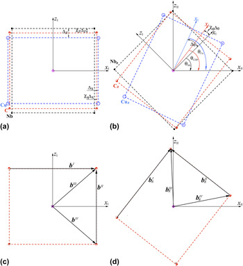
(i) Construct a trial reference lattice. As schematically shown in Fig. 2, if an interface does not involve a twist, two unknown variables χ x and χ z correspond to the geometric partition of the mismatch strain between the two crystals in the two commensurate directions. If a twist is involved in creating an interface, the third variable χ θ is introduced to describe the partition of the twist angle between the two crystals.
FIG. 2.(a) A Commensurate/Coherent Dichromatic Pattern (CDP) and natural dichromatic patterns (NDPs) between Cu and Nb. (b) the Rotation CDP (RCDP) and the corresponding NDPs. (c) Possible Burgers vectors in the CDP lattice, and (d) Possible Burgers vectors in the RCDP lattice. Three variables are employed to describe the CDP and RCDP lattices with respect to the NDPs.

(ii) According to the trial reference lattice, we first calculate the two distortion matrices S A, S B, and the inverse matrices S A−1 and S B−1.
(iii) We assign the possible lines to be interface dislocation lines according to atomistic simulations. For each line, the line sense could be positive or negative, and its Burgers vector can be one or a combination of the lattice vectors in the trial reference lattice.
(iv) If there are only two sets of lines presented within the simulated interface, we assume two sets of interface dislocations. Using the F-B theory, more than one set of solutions can be found. The real solution must be one that fully satisfies the prediction from atomistic simulations. In other words, the line senses and the spacings of interface dislocations should be consistent with the disregistry analysis of the atomistic simulated interfaces, and the Burgers vector must be a vector in the reference lattice.
(v) If all solutions cannot satisfy the disregistry analysis of the atomistic simulated interfaces, we then adjust the three variables, χ z, χ z and χ θ until the solutions are consistent with the disregistry analysis of the atomistic simulated interfaces.
(vi) Corresponding to the F-B theory for a flat interface, there are only two independent probe vectors (orthogonal), because any probe vector lying in the interface can be described with the two vectors. In other words, there are only four governing equations with respect to the two independent probe vectors (four terms in the matrix. However, there are more than four unknown variables: χ x, χ z, χ θ, ξ i, b i, d i, and N. If there are more than two dislocation lines presented within the atomic interface, the F-B equations cannot be directly solved. First, we assign the line sense and Burgers vector to one of all lines that are characterized from atomistic simulations. Then using the F-B equation, we search for the possible line sense and Burgers vector for the other two lines. If there does not exist any solution in agreement with atomistic simulations, we will re-assign the line sense and Burgers vector for the line and repeat the above procedure.

III. APPLICATION OF AIFB FOR CHARACTERIZING INTERFACE DISLOCATIONS
Two typical interfaces are studied to demonstrate the AIFB. The two interfaces are bonded between fcc {110} and bcc {001}. The BUCs in the two crystallographic planes are similar and could form semicoherent interfaces (Fig. 2). The 1st interface only contains the misfit dislocations because of the parallelism of their commensurate directions. The 2nd interface destroys the parallelism through twisting one crystal relative to the other about the interface normal and thus contains the additional twist angle with respect to the 1st one. Thus, the 1st interface can be used to determine the two parameters χ x and χ z related to the partition of the mismatch strain, and the 2nd interface can be used to determine the third parameter χ θ related to the partition of the twist angle.
Atomistic simulations were performed for the two interfaces between the dissimilar crystals, copper (Cu), and niobium (Nb), with embedded atom method (EAM) interatomic potentials.Reference Wang, Hoagland, Hirth and Misra35–Reference Demkowicz and Hoagland38 These potentials have been demonstrated to reproduce well measurements for surface diffusion, defect formation energies, crystal growth during physical vapor deposition.Reference Liu, Hoagland, Wang, Germann and Misra37–Reference Wang, Huang, Kesapragada and Gall41
A. Interface geometries: CDP and RCDP lattices
The 1st interface is bonded between fcc  $\left( {\bar 1\bar 10} \right)$ and bcc (001), and within the interface plane [001]Cu||[010]Nb parallel to the x-axis and
 $\left. {\left[ {1\bar 10} \right]_{Cu} } \right\|\left[ {100} \right]_{Nb}$ parallel to the z-axis. Corresponding to
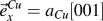 $\vec e_x^{Cu} = a_{Cu} \left[ {001} \right]$,
 $\vec e_x^{Nb} \left[ {010} \right] = a_{Nb} \left[ {010} \right]$,
 $\vec e_z^{Cu} = {\textstyle{{a_{Cu} } \over 2}}\left[ {1\bar 10} \right]$, and
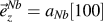 $\vec e_z^{Nb} = a_{Nb} \left[ {100} \right]$, using Eq. (3), we found
 $\left( {N_x^{Cu} ,N_x^{Nb} } \right)$ = (21, 23) and
 $\left( {N_z^{Cu} ,N_z^{Nb} } \right)$= (31, 24), and the imposed strains
 $\left( {\varepsilon _{xx}^{Cu} ,\varepsilon _{zz}^{Cu} } \right)$ = (1.6E-5, -1.5E-4) for Cu and
 $\left( {\varepsilon _{xx}^{Nb} ,\varepsilon _{zz}^{Nb} } \right)$ = (-2.9E-5, 1.4E-4) for Nb. The strained-NDP has the final dimensions 7.59 and 7.92 nm in the x and z directions corresponding to a super BUC at equilibrium.
The 2nd interface is also bonded between fcc  $\left( {\bar 1\bar 10} \right)$ and bcc (001) with the Nishiyama-Wasserman (NW) orientation relationship. Within the interface plane,
 $\left. {\left[ {\bar 111} \right]_{Cu} } \right\|\left[ {1\bar 10} \right]_{Nb}$ is parallel to the x-axis and
 $\left. {\left[ {1\bar 12} \right]_{Cu} } \right\|\left[ {110} \right]_{Nb}$ is parallel to the z-axis. Corresponding to
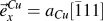 $\vec e_x^{Cu} = a_{Cu} \left[ {\bar 111} \right]$,
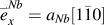 $\mathord{\buildrel{\lower3pt\hbox{$\scriptscriptstyle\rightharpoonup$}}\over e} _x^{Nb} = a_{Nb} \left[ {1\bar 10} \right]$,
 $\vec e_z^{Cu} = {\textstyle{{a_{Cu} } \over 2}}\left[ {1\bar 12} \right]$, and
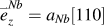 $\mathord{\buildrel{\lower3pt\hbox{$\scriptscriptstyle\rightharpoonup$}}\over e} _z^{Nb} = a_{Nb} \left[ {110} \right]$, using Eq. (3) we found
 $\left( {N_x^{Cu} ,N_x^{Nb} } \right)$ = (23, 31) and
 $\left( {N_z^{Cu} ,N_z^{Nb} } \right)$ = (18, 17), and the imposed strains
 $\left( {\varepsilon _{xx}^{Cu} ,\varepsilon _{zz}^{Cu} } \right)$ = (2.4E-3, -2.0E-3) for Cu and
 $\left( {\varepsilon _{xx}^{Cu} ,\varepsilon _{zz}^{Cu} } \right)$ = (-2.4E-3, 2.1E-3) for Nb. The strained-NDP has the final dimensions 14.44 and 7.93 nm in the x and z directions corresponding to a super BUC at equilibrium.
Figures 2(a) and 2(b) show the natural lattices and the reference lattices of the 1st and 2nd interfaces, respectively. The reference lattice (CDP) contains two variables χ x and χ z that describe the partition of the geometry mismatch of the neighboring lattice sites. It is noticed that the 2nd interface can be obtained by twisting the two crystals θ Cu = 54.74° for Cu and θ Nb = 45° for Nb around the interface normal. We speculated that the 2nd interface will share the same reference lattice but it will be rotated about θ CDP[= θ Nb + χ θ(θ Cu − θ Nb)]. Corresponding to the twist, the reference lattice in the 2nd interface is called rotation CDP lattice (RCDP).
For the 1st interface [Fig. 2(a)], we define the two variables, χ x and χ z, and the reference lattice (CDP). The four sites in the CDP lattice can be written in the x-z coordinate system as
 $$\eqalignb{ C( 1 ) = ( {{{a_{Nb} } \over 2} + \chi _x ( {{{a_{Cu} } \over 2} - {{a_{Nb} } \over 2}} )\quad, {{a_{Nb} } \over 2} - \chi _z ( {{{a_{Nb} } \over 2} - {{\sqrt 2 a_{Cu} } \over 4}} ) )\quad,C( 2 ) = ( { - {{a_{Nb} } \over 2} - \chi _x ( {{{a_{Cu} } \over 2} - {{a_{Nb} } \over 2}} )\quad,\quad {{a_{Nb} } \over 2} - \chi _z ( {{{a_{Nb} } \over 2} - {{\sqrt 2 a_{Cu} } \over 4}} ) )\quad,C( 3 ) = ( { - {{a_{Nb} } \over 2} - \chi _x ( {{{a_{Cu} } \over 2} - {{a_{Nb} } \over 2}} )\quad,\quad - {{a_{Nb} } \over 2} + \chi _z ( {{{a_{Nb} } \over 2} - {{\sqrt 2 a_{Cu} } \over 4}} ) )\quad, C( 4 ) = ( {{{a_{Nb} } \over 2} + \chi _x ( {{{a_{Cu} } \over 2} - {{a_{Nb} } \over 2}} )\quad,\quad - {{a_{Nb} } \over 2} + \chi _z ( {{{a_{Nb} } \over 2} - {{\sqrt 2 a_{Cu} } \over 4}} ) )\quad. \cr}$$
The corresponding lattice sites in Cu are
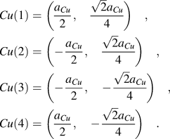 $$\eqalignb{ & Cu\left( 1 \right) = \left( {{{a_{Cu} } \over 2},\quad {{\sqrt 2 a_{Cu} } \over 4}} \right)\quad, \cr & Cu\left( 2 \right) = \left( { - {{a_{Cu} } \over 2},\quad {{\sqrt 2 a_{Cu} } \over 4}} \right)\quad, \cr & Cu\left( 3 \right) = \left( { - {{a_{Cu} } \over 2},\quad - {{\sqrt 2 a_{Cu} } \over 4}} \right)\quad, \cr & Cu\left( 4 \right) = \left( {{{a_{Cu} } \over 2},\quad - {{\sqrt 2 a_{Cu} } \over 4}} \right)\quad. \cr}$$
and in Nb are
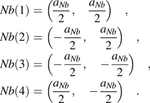 $$\eqalignb{ & Nb\left( 1 \right) = \left( {{{a_{Nb} } \over 2},\quad {{a_{Nb} } \over 2}} \right)\quad, \cr & Nb\left( 2 \right) = \left( { - {{a_{Nb} } \over 2},\quad {{a_{Nb} } \over 2}} \right)\quad, \cr & Nb\left( 3 \right) = \left( { - {{a_{Nb} } \over 2},\quad - {{a_{Nb} } \over 2}} \right)\quad, \cr & Nb\left( 4 \right) = \left( {{{a_{Nb} } \over 2},\quad - {{a_{Nb} } \over 2}} \right)\quad. \cr}$$
The distortion matrix is constructed by mapping the lattice vectors from the real lattices to the reference lattice as follows.
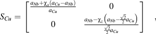 $$S_{Cu} = \left[ {\matrix{ {{{a_{Nb} + \chi _x \left( {a_{Cu} - a_{Nb} } \right)} \over {a_{Cu} }}} & 0 \cr 0 & {{{a_{Nb} - \chi _z \left( {a_{Nb} - {{\sqrt 2 } \over 2}a_{Cu} } \right)} \over {{{\sqrt 2 } \over 2}a_{Cu} }}} \cr } } \right]\quad,$$
 $$S_{Nb} = \left[ {\matrix{ {{{a_{Nb} + \chi _x \left( {a_{Cu} - a_{Nb} } \right)} \over {a_{Nb} }}} & 0 \cr 0 & {{{a_{Nb} - \chi _z \left( {a_{Nb} - {{\sqrt 2 } \over 2}a_{Cu} } \right)} \over {a_{Nb} }}} \cr } } \right]\quad.$$
The possible Burgers vectors defined in the CDP lattice [Fig. 2(c)] are
 $$\eqalign{ & b^I = \left[ {a_{Nb} + \chi _x \left( {a_{Cu} - a_{Nb} } \right),0} \right]\quad, \cr & b^{II} = \left[ {0,a_{Nb} - \chi _z \left( {a_{Nb} - {{\sqrt 2 } \over 2}a_{Cu} } \right)} \right]\quad, \cr & b^{III} = \left[ {{{a_{Nb} + \chi _x \left( {a_{Cu} - a_{Nb} } \right)} \over 2},{{a_{Nb} - \chi _z \left( {a_{Nb} - {{\sqrt 2 } \over 2}a_{Cu} } \right)} \over 2}} \right]\quad, \cr & b^{IV} = \left[ {{{a_{Nb} + \chi _x \left( {a_{Cu} - a_{Nb} } \right)} \over 2},{{ - a_{Nb} + \chi _z \left( {a_{Nb} - {{\sqrt 2 } \over 2}a_{Cu} } \right)} \over 2}} \right] \,\,\,.\cr}$$
For the 2nd interface [Fig. 2(b)], as it is related to the twist one of the 1st interface, the reference lattice will share the same reference lattice as that in the 1st interface but it will be rotated θθCDP about the normal of the interface. Thus, a third variable χ θ is introduced to describe the RCDP. Corresponding to Fig. 2(b), the four lattice sites in the RCDP lattice can be written in the x-z coordinate as
 $$C_R \left( i \right) = \left[ {\matrix{ {\cos \left( {\theta _{Nb} + \chi _\theta \left( {\theta _{Cu} - \theta _{Nb} } \right)} \right)} & {\sin \left( {\theta _{Nb} + \chi _\theta \left( {\theta _{Cu} - \theta _{Nb} } \right)} \right)} \cr { - \sin \left( {\theta _{Nb} + \chi _\theta \left( {\theta _{Cu} - \theta _{Nb} } \right)} \right)} & {\cos \left( {\theta _{Nb} + \chi _\theta \left( {\theta _{Cu} - \theta _{Nb} } \right)} \right)} \cr } } \right]C\left( i \right)\quad.$$
The corresponding lattice sites in Cu are
 $$Cu_R \left( i \right) = \left[ {\matrix{ {\cos \left( {\theta _{Cu} } \right)} & {\sin \left( {\theta _{Cu} } \right)} \cr { - \sin \left( {\theta _{Cu} } \right)} & {\cos \left( {\theta _{Cu} } \right)} \cr } } \right]Cu\left( i \right)\quad.$$
and in Nb are
 $$Nb_R \left( i \right) = \left[ {\matrix{ {\cos \left( {\theta _{Nb} } \right)} & {\sin \left( {\theta _{Nb} } \right)} \cr { - \sin \left( {\theta _{Nb} } \right)} & {\cos \left( {\theta _{Nb} } \right)} \cr } } \right]Nb\left( i \right)\quad.$$
The distortion matrixes S R,Cu and S R,Nb are constructed by mapping the lattice vectors from the real lattices to the RCDP, containing one more unknown variable, χ θ. The four Burgers vectors defined in the RCDP lattice [Fig. 2(d)] are
 $$b_R^i = \left[ {\matrix{ {\cos \left( {\theta _{Nb} + \chi _\theta \left( {\theta _{Cu} - \theta _{Nb} } \right)} \right)} & {\sin \left( {\theta _{Nb} + \chi _\theta \left( {\theta _{Cu} - \theta _{Nb} } \right)} \right)} \cr { - \sin \left( {\theta _{Nb} + \chi _\theta \left( {\theta _{Cu} - \theta _{Nb} } \right)} \right)} & {\cos \left( {\theta _{Nb} + \chi _\theta \left( {\theta _{Cu} - \theta _{Nb} } \right)} \right)} \cr } } \right]b^i ,\quad i\, = \,{\rm{I}},{\rm{II}},{\rm{III}},\;{\rm{and}}\;{\rm{IV}}\quad.$$
With these possible Burgers vectors and the distortion matrixes, the characters of discrete interface dislocations including the Burgers vectors, the line senses, and the spacing can be obtained by solving the F-B equations when varying the three variables. The iteration regarding the reference lattice stops when the solutions obtained by solving the F-B equations are identical with the prediction from atomistic simulations.
B. Interface dislocations and the CDP lattice in the 1st interface
Atomic structures of the unrelaxed and relaxed interface structures are shown in Figs. 3(a) and 3(b), respectively. The disregistry plot of the vector fields  $r_{ij}^{R - U}$ is shown in Fig. 3(c), which is independent on the choice of the reference lattice. First, a quasirepeating pattern observed in Figs. 3(b) and 3(c) describes a two-dimensional BUC in the shape of a rectangle. Second, inside the rectangle, atomic structures are close to a coherent lattice. The displacement patterns associated with these distorted fields perturb the locations of nearby atoms as would be expected of a crystalline defect with a well-defined elastic strain field, as indicated by the solid lines. Third, the highly distorted regions correspond to the corners of the rectangle and the intersection points of solid lines in Figs. 3(b) and 3(c). According to the characteristics of the displacement of a dislocation, the interface dislocations should be aligned to these solid lines.
Atomic structures of (a) the unrelaxed and (b) relaxed interfaces between Cu and Nb. (c) The disregistry plot of the vector fields  $r_{ij}^{R - U}$. The length of arrows indicates the magnitude of the displacements, and the color is assigned with respect to the direction of the displacement. The green lines indicate the interface dislocations.

To quantitatively identify interface discrete dislocations, we performed the disregistry analysis as described in Sec. II. Figure 4(a) shows the disregistry vectors  $r_{ij}^{R - C}$ and
 $r_{ij}^{U - C}$ as the probe vector is located at z = 0 along the x-direction. Figure 4(b) shows the disregistry
 $r_{ij}^{R - U}$ corresponding to the difference between the two disregistry vectors
 $r_{ij}^{R - C}$ and
 $r_{ij}^{U - C}$ in Fig. 4(a). Figure 5(a) shows the disregistry vectors
 $r_{ij}^{R - C}$ and
 $r_{ij}^{U - C}$ as the probe vector is located at x = 0 along the z-direction. Figure 5(b) shows the disregistry
 $r_{ij}^{R - U}$ along the z-direction corresponding to the difference between the two disregistry vectors
 $r_{ij}^{R - C}$ and
 $r_{ij}^{U - C}$ in Fig. 5(a). These disregistry plots provide the useful information in understanding the interface relaxation and determining the position of interface discrete dislocations. First, the disregistry corresponding to the vector
 $r_{ij}^{U - C}$ shows a uniform distribution of interface Burgers vectors contents, but the vector
 $r_{ij}^{R - C}$ corresponds to a nonuniform distribution of interface Burgers vectors content. The nonuniform distribution is a result of the formation of interface discrete dislocations, corresponding to the recombination of the continuous distribution of interface Burgers content, and indicating the number of interface discrete dislocations that intersect with the probe vector. Second, the disregistry
 $r_{ij}^{R - U}$ only shows the nonuniform relaxation in association with the formation of interface discrete dislocations. Corresponding to Figs. 4 and 5 with respect to the two probe vectors, the interface dislocation will locate at the position where the disregistry
 $r_{ij}^{R - C}$experiences the change of the sign from the negative to the positive or from the positive to the negative, depending on the sign of Burgers vector and the corresponding line sense. The similar plots as Figs. 4 and 5 can be drawn when the probe vectors are located at any different position; the results show the same position as that in Figs. 4 and 5. The location and the sense of interface discrete dislocation lines then can be defined by connecting these positions that are defined with respect to the probe vectors. With this disregistry analysis, interface discrete dislocation pattern can be visualized in the disregistry plot of the vector field
 $r_{ij}^{R - U}$ in Fig. 3(c). Third, as a result, two sets of edge-type dislocations are identified in Figs. 3–5. The set 1 dislocation line is parallel to the x-axis and the set 2 parallel to the z-axis, whereas the average spacing between the same type interface discrete dislocations are calculated to be 1.279 nm for the set 1 and 3.328 nm for the set 2. In addition, the further information regarding the core width of interface dislocations can also be calculated from the first-order derivation of the vector
 $r_{ij}^{R - C}$with respect to the coordinate.
Identification of interface dislocations. (a) The disregistry vectors  $r_{ij}^{R - C}$ and
 $r_{ij}^{U - C}$ as the probe vector is located at z = 0 along the x-direction. (b) The disregistry
 $r_{ij}^{R - U}$ corresponding to the difference between the two disregistry vectors
 $r_{ij}^{R - C}$and
 $r_{ij}^{U - C}$ in (a). r ij,x and r ij,z present the x-component and the z-component of the disregistry vector. The positions of interface dislocations are marked as a dislocation symbol.

Identification of interface dislocations. (a) The disregistry vectors  $r_{ij}^{R - C}$ and
 $r_{ij}^{U - C}$ as the probe vector is located at x = 0 along the z-direction. (b) The disregistry
 $r_{ij}^{R - U}$ corresponding to the difference between the two disregistry vectors
 $r_{ij}^{R - C}$ and
 $r_{ij}^{U - C}$ in (a). r ij,x and r ij,z present the x-component and the z-component of the disregistry vector. The positions of interface dislocations are marked as a dislocation symbol.

Corresponding to the analysis of atomistic simulations, the interface contains two sets of interface dislocations, that is N = 2; the line senses are ξ 1 = [001] for the set 1 dislocation and ξ 2 = [100] for the set 2 dislocation in the x-y-z coordinates, and the average spacings are d 1 = 3.80 nm and d 2 = 1.13 nm, respectively. Thus there are the four unknown variables χ x, χ z, b 1, and b 2. For the first attempt, we simply assign χ x = χ z = 0.5, and choose the two probe vectors along the x-axis and z-axis in the BUC, the results obtained by solving the F-B Eq. (2) indicate that both sets should be pure-edge dislocations, thus  $b_{{\rm{intf}}}^I = b^I$ and
 $b_{{\rm{intf}}}^{II} = b^{II}$. After this step, there are only two unknown variables χ x and χ z. By solving F-B Eq. (2), we obtained χ x = 0.48 and χ z = 0.54, implying a nonequal partition of the mismatch strain between the two crystals. Correspondingly, the CDP and the four lattice vectors are determined using Eqs. (4) and (9).
C. Interface dislocations and the RCDP lattice in the 2nd interface
Atomic structures of the unrelaxed and relaxed structures of the 2nd interface are shown in Figs. 6(a) and 6(b), respectively. The disregistry plot of the vector field  $r_{ij}^{R - U}$ is shown in Fig. 6(c). It is clearly observed that the regions surrounded by the distorted regions take the coherent structure. Following the same method in Sec. III. B, we outline interface dislocations as the dashed lines in Fig. 6. It is noticed that the two sets of dislocations within the interface are not straight, instead forming a segmented pattern. Corresponding to the feature revealed by the disregistry analysis in Fig. 6(c), we hypothesize that the segmented pattern results from the reaction of the two sets of dislocations, which will be demonstrated using discrete dislocation dynamics in a later section. Thus, the interface will contain two sets of dislocations and they are not simply parallel to either the x-axis or the z-axis.
Atomic structures of (a) the unrelaxed and (b) relaxed interfaces between Cu and Nb. (c) The disregistry plot of the vector fields  $r_{ij}^{R - U}$. The length of arrows indicates the magnitude of the displacements, and the color is assigned with respect to the direction of the displacement. The green and yellow lines indicate the interface dislocations.

To quantitatively determine the discrete interface dislocations, Fig. 7(a) shows the disregistry vectors  $r_{ij}^{R - C}$ and
 $r_{ij}^{U - C}$ when the probe vector is located at x = 0 along the z-direction; Fig. 7(b) shows the disregistry
 $r_{ij}^{R - U}$ corresponding to the difference between the two disregistry vectors
 $r_{ij}^{R - C}$ and
 $r_{ij}^{U - C}$ in Fig. 7(a). As discussed in Sec. III. B, there are two dislocations in a unit cell, denoted as
 $b_{{\rm{intf}}}^I$. Figure 8(a) shows the disregistry vectors
 $r_{ij}^{R - C}$ and
 $r_{ij}^{U - C}$ as the probe vector is located at z = 0 along the x-direction. Figure 8(b) shows the disregistry
 $r_{ij}^{R - U}$ along the z-direction corresponding to the difference between the two disregistry vectors
 $r_{ij}^{R - C}$ and
 $r_{ij}^{U - C}$ in Fig. 8(a). As shown in Fig. 8(b), there are eight discrete dislocations, denoted as
 $b_{{\rm{intf}}}^{II}$. To determine the line direction of the discrete dislocation, the disregistry analysis was performed with respect to the position of the probe vector. Figure 9 show the disregistry
 $r_{ij}^{R - U}$ as the probe vector is located at x = 6 nm along the z-direction, conforming to the existence of the two discrete dislocations
 $b_{{\rm{intf}}}^I$ and their positions. Using the same method, the position of discrete dislocations
 $b_{{\rm{intf}}}^{II}$ can be determined with respect to the location of the probe vector along the x-direction. By connecting these positions determined through the above analysis, we found that the line of the dislocation
 $b_{{\rm{intf}}}^I$ is parallel to the vector [cos(28.9°) 0 sin(28.9°)], and the line of dislocation
 $b_{{\rm{intf}}}^{II}$ is parallel to the vector [cos(77.2°) 0 sin(77.2°)], which is defined by connecting the middle points of each segment.
Identification of interface dislocations. (a) The disregistry vectors  $r_{ij}^{R - C}$ and
 $r_{ij}^{U - C}$ as the probe vector is located at x = 0 along the z-direction. (b) The disregistry
 $r_{ij}^{R - U}$ corresponding to the difference between the two disregistry vectors
 $r_{ij}^{R - C}$ and
 $r_{ij}^{U - C}$ in (a). r ij,x and r ij,z present the x-component and the z-component of the disregistry vector. The positions of interface dislocations are marked as a dislocation symbol.

Identification of interface dislocations. (a) The disregistry vectors  $r_{ij}^{R - C}$ and
 $r_{ij}^{U - C}$ as the probe vector is located at z = 0 along the x-direction. (b) The disregistry
 $r_{ij}^{R - U}$ corresponding to the difference between the two disregistry vectors
 $r_{ij}^{R - C}$ and
 $r_{ij}^{U - C}$ in (a). r ij,x and r ij,z present the x-component and the z-component of the disregistry vector. The positions of interface dislocations are marked as dislocation symbols.

Identification of interface dislocations. (a) and (b) The two components of the disregistry  $r_{ij}^{R - U}$ corresponding to the difference between the disregistry vectors
 $r_{ij}^{R - C}$ and
 $r_{ij}^{U - C}$ as the probe vector is located at x = 6 nm along the z-direction. r ij,x and r ij,z present the x-component and the z-component of the disregistry vector. The positions of interface dislocations are marked as dislocation symbols.

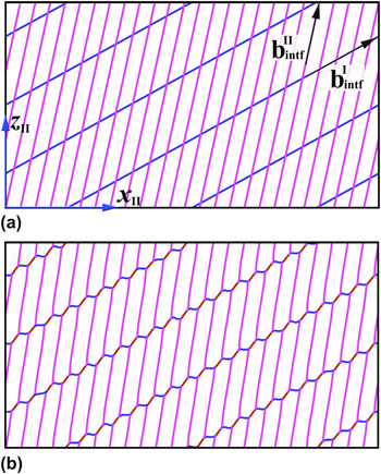
Demonstration of local reactions of interface dislocations. (a) The initial pattern of two sets of interface dislocations, and (b) the relaxed, equilibrium dislocation pattern obtained by PDD simulations.

From atomistic simulations, we find that the interface contains two sets of interface dislocations, N = 2. For set 1, the line sense is [cos(28.9°) 0 sin(28.9°)] and the average spacing is d 1 = 7.0 nm; for the set 2, the line sense is along [cos(77.2°) 0 sin(77.2°)] and d 2 = 1.8 nm. As before for the first attempt, we assign χ θ = 0.5 and choose the two probe vectors along the x-axis and the z-axis in the simulation cell. The results obtained by solving the F-B Eq. (2) indicate that the Burgers vector associated with set 1 interface dislocation is close to  $- b_R^I$ and with set 2 interface dislocation is close to a combination of
 $2b_R^{II} + b_R^I$. By optimizing χ θ to minimize the difference of the net Burgers vector within interface, we found that χ θ = 0.45, which implies a nonequal partition of the twist angle between the two crystals.
We further examined the local reaction of two sets of interface dislocations using the Parameterized Dislocation Dynamics (PDD) developed by Nasr Ghoniem et al.Reference Ghoniem, Tong and Sun42 In the PDD simulations, for simplicity, we assume an isotropic medium. Figure 10(a) shows the initial pattern of two sets of interface dislocations. The line directions and Burgers vectors of dislocations were initially set the same as those from the atomistic analysis. A relaxation calculation was performed to equilibrate the dislocation microstructure. The evolution of the dislocation structure is only driven by the dislocation interaction stresses. The calculation is interrupted when no significant dislocation motion is observed over a long time period. The relaxed, equilibrium dislocation pattern in Fig. 10(b) is consistent with that observed in the atomistic simulations.
IV. CONCLUSIONS
For characterizing interface dislocations in semicoherent interface, we propose an AIFB to determine interface dislocations by combining the classical Frank-Bilby theory and atomistic simulations. This method can overcome the shortcomings in choosing the reference lattice in the F-B theory and in determining the Burgers vectors of interface dislocations in molecular dynamics (MD) simulations. We demonstrated our method by characterizing two atomically flat interfaces, one only involves a lattice mismatch and the other additionally involves a twist with respect to the first interface. The results revealed that (i) both interfaces share the same reference lattice, CDP; (ii) the Burgers vectors of the interface dislocations can be well defined in the reference lattice (CDP or RCDP). (iii) These Burgers vectors always differ, sometimes only slightly, from the Burgers vectors of either crystal adjoining the interface in its perfect state. Most importantly, (iv) the CDP (lattice) is not simply a geometric average of the two lattices, implying a nonequal partition of the lattice misfit. If a twist is also present in the interface, the partition of the twist is also nonequal between the two lattices.
ACKNOWLEDGMENTS
This work was supported by the Center for Materials at Irradiation and Mechanical Extremes, an Energy Frontier Research Center funded by the U.S. Department of Energy, Office of Science, Office of Basic Energy Sciences under Grant No. 2008LANL1026. JW and IJB also thank the support provided by a Los Alamos National Laboratory Directed Research and Development project ER20110573 and DR20110029. CZZ thanks the support provided by CNLS at Los Alamos National Laboratory.