Introduction
Optical techniques based on digital cameras are increasingly used to measure surface displacements or strains on a sample under loading. In general, this requires some form of a pattern on the sample's surface to track deformations in two-dimensional space with one digital camera and in three-dimensional space with two or more digital cameras. The out of plane displacement component (in the third dimension) is quantified using computer vision techniques. Among the displacement-tracking algorithms, the pure grid method appears to be the simplest as it utilizes a uniform grid pattern. The displacements are evaluated on the nodes and strains are computed from displacement gradients using the strain displacement relation:  ${\bf \varepsilon} = 0.5\,((\nabla {\bf u}) + (\nabla {\bf u})^{\rm T})$ where
 ${\bf \varepsilon} $ denotes the strain tensor and
 ${\bf u}$ denotes the displacement vector. Digital image correlation (DIC) methods utilize random speckle (dot) patterns,[Reference Bruck, McNeill, Sutton and Peters1] decompose the problem domain into a mesh consisting of grid points and facets. The displacements are calculated from facet similarities/correlations between deformed and undeformed images. DIC systems are commercially as well as open source available, while the latter ones are mostly confined to two-dimensional capabilities. Researchers at the Naval Research Laboratories led by Dr. John Michopoulos introduced a mesh-free random grid method that also relies on random speckle patterns, but does not require facets.[Reference IIiopoulos, Michopoulos, Orifici and Thomson2, Reference Michopoulos and IIiopoulos3] Instead, centroids of speckles are identified and their displacements between pre- and post-deformed images are calculated. Digital strain imaging was developed by the same group and quantifies strains directly from the speckle pattern,[Reference IIiopoulos and Michopoulos4] resulting in lower strain noise levels as opposed to calculating them via noisy displacement differentiation.
Displacement or strain measurements based on digital cameras provide opportunities to improve the mechanical characterization of solids. For example, uniaxial tensile tests are currently used to characterize a material's stress–strain behavior. This, however, is a crude approach since (1) the tensile testing device has some play in the fixture (rigid body motion) and is falsely recorded as elongation (or stretch) of the specimen, (2) slip may occur resulting in non-axial loading conditions, and (3) local strains due to necking are significantly different from averaged recorded strains. Measuring strains using one of the aforementioned techniques would address all these issues.[Reference Stamborska, Kvícala and Losertova5, Reference Kato6] The authors of this paper took this one step further and utilized boundary displacements to map the model parameters of a material with varying parameter distribution by solving an inverse problem in elasticity.[Reference Mei, Fulmer, Raja, Wang and Goenezen7, Reference Mei, Wang, Shen, Rabke and Goenezen8] This has a potential in characterizing engineered tissues, monitoring growth and remodeling of tissues, characterizing additively manufactured materials, and analyzing collective cell expressions locally that are all associated with changes in the stiffness distribution in space. Measurements were simulated using finite element methods, and the problem domain was confined to two dimensions to reduce computational time when solving the inverse problem. Further, we assumed a linear elastic and incompressible material behavior under plane strain conditions. Simulated displacement measurements were assumed to be known solely on boundary edges (assuming plane strain conditions) and the shear moduli were introduced as unknowns on finite element mesh nodes and interpolated throughout the domain with linear shape functions. Thus, the total number of unknown shear moduli was equal to the mesh size, i.e., total number of nodes. No assumptions were made on locally homogeneous regions as was done in other works.[Reference Liu, Sun, Wang and Vannier9–Reference Elijah, Houten, Peters and Chase11]
Since the authors of this paper demonstrated proof of concept in prior works for two-dimensional problem domains composed of one and two stiff inclusions in a homogeneous background, one may raise the question if this procedure may work for a large number of stiff inclusions. Further, it is not obvious that this methodology could actually work for three-dimensional problems using surface displacement measurements as well. We acknowledge that the total number of unknown shear moduli increases dramatically for the problem domain in three-dimensional space. To the best of our knowledge, in this paper, we demonstrate for the first time that it is feasible to recover (1) inclusions with varying stiffness values and diameters, (2) nine stiff inclusions embedded in a homogeneous background, and (3) the shear modulus distribution for a three-dimensional problem domain using solely boundary displacement measurements and without any a priori assumptions about the shear modulus distribution. A thorough literature review on related works, but using prior information on the shear modulus distribution was provided in.[Reference Mei, Fulmer, Raja, Wang and Goenezen7] Key ingredients that allow the successful solution of the inverse problem with limited measurements on the specimen's surface are the (a) inverse problem formulation posed as a constrained minimization problem, (b) regularization term in the objective function to smooth the overall reconstruction and control how close the measured displacements fit the computed displacements, (c) accommodation of multiple measurements (from multiple experiments) in the objective function to yield a unique solution, and (d) the efficient computation of the gradient for the optimization scheme using the adjoint equations. Overall, the methodology presented in this paper could have a great impact and help researchers characterize in vitro samples, since it requires low-cost digital cameras for data acquisition.
Methods
We assume the material to be isotropic, non-homogeneous, and linear elastic. We apply forces in the form of indentations to gently deform the problem domain and utilize boundary deformations to solve an inverse problem, discussed in more detail below. Acquisition of boundary displacement measurements will be simulated with finite element methods.[Reference Reddy12] For the two-dimensional problems, we will assume plane strain conditions of an incompressible material. For the three dimensional problem, we will assume that the material is incompressible as well, since many soft tissues or engineered tissues are known to be nearly incompressible. The inverse problem is posed as a constrained optimization problem, where the equilibrium equations in elasticity represent the constraint of the problem. In more detail, given N measured boundary displacement data sets, we seek to find the optimal shear modulus distribution μ such that the objective function:
 $$\eqalign{ \pi& = \sum\limits_{i = 1}^N {\left[ {\sum\limits_{e = 1}^{n_n} {\int\limits_{\Omega _e} {{\left( {\sum\limits_{\,j = 1}^{n_e} {N_j^e ({\bf x}){\left( {{\bf u}_e^i - {({\bf u}_e^i )}_{{\rm meas}}} \right)}_j}} \right)}^2d\Omega}}} \right]} \cr &\quad + \alpha \sum\limits_{e = 1}^{n_n} {\int\limits_{\Omega _e} {\sqrt {\sum\limits_{\,j = 1}^{n_e} { \vert \mu _j^e \nabla N_j^e ({\bf x}) \vert ^2} + c_0^2}}} \,d\Omega} $$
is minimized, subject to the constraint of the equilibrium equations as detailed further below. The objective function is provided in discretized form using finite element shape functions  $N_j^e ({\bf x})$ for the e-th element and j-th local node number. In Eq. (1), n e and n n are the number of nodes on element e and the total number of elements throughout the entire problem domain, respectively. The first term is referred to as the boundary displacement correlation term, where
 ${\bf u}_e^i $ and
 $({\bf u}_e^i )_{{\rm meas}}$ are the i-th computed and measured boundary displacement datasets, respectively, and we set
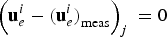 $\left( {{\bf u}_e^i - {({\bf u}_e^i )}_{{\rm meas}}} \right)_j\; = 0$ if it is not on the measured boundary. We emphasize that it is important to conduct a large number of experiments denoted by N in order to drive the recovered shear modulus distribution to a unique solution. The computed displacements
 ${\bf u}_e^i $ satisfy the equations of equilibrium, solved with finite element methods, and referred to as the forward problem. We note that
 ${\bf u}_e^i $ also depends on the shear modulus distribution. To simplify the implementation and make use of the currently existing in-house written program structure, we define the first integral in Eq. (1) over finite element volumes Ωe at measured boundaries rather than using boundary (surface) elements directly. Consequently, shape functions
 ${\bf N}_{}^e $ are defined over Ωe at the boundary; however, no measurements from the domain's interior are utilized. This has been thoroughly discussed in[Reference Mei, Fulmer, Raja, Wang and Goenezen7] and therein concluded that it introduces different weights in correlating measured and computed displacements.
Ideally, the boundary displacement correlation term should be as close as possible to a zero value after solving the minimization problem. However, due to noise in measured boundary displacements  $({\bf u}_e^i )_{{\rm meas}}$, we do not wish to fit this term beyond inherent noise level. Since the inverse problem is highly ill-posed, this would manifest itself in dramatically amplified noise levels in the recovered shear modulus distribution. We address this issue with a so-called regularization term in the second term of the objective function, and select the total variation diminishing regularization that penalizes oscillations in the shear modulus distribution and smooths the overall solution. In Eq. (1), this regularization term is provided in discretized form with the nodal shear modulus
 $\mu _j^e $, a constant c 0 = 0.01 to avoid singularities when differentiating, and the regularization factor α. The regularization factor α assigns a weight to the regularization term and with that its relative contribution to the boundary displacement correlation term. We select the regularization factor such that the boundary displacement correlation term is not smaller than the actual noise level. Later in the “Two-dimensional problem domain with two inclusions of different sizes and shear modulus values” section, we rewrite the displacement correlation term by scaling it with measured displacements, take the square root, and require this to be of the order of the relative noise in the displacement. This is also known as Morozov's discrepancy principle[Reference Frick, Lorenz and Resmerita13] and given that our group has extensive experience with these computations, the actual regularization factors were selected after few trial and errors.
The inverse problem is solved using a quasi-Newton method, more precisely, the limited Broyden–Fletcher–Goldfarb–Shanno method detailed in.[Reference Zhu, Byrd, Lu and Nocedal14] This requires the calculation of the gradient of the objective function with respect to the shear moduli. We calculate the gradient efficiently using the adjoint method and the interested reader is referred to[Reference Goenezen15, Reference Goenezen, Barbone and Oberai16] for a thorough derivation. The constrained minimization procedure is considered to be converged when the relative change in the objective function or the gradient is close to machine precision.
Finally, the computations were done on Ada, an IBM X86_64 cluster hosted and maintained by the High Performance Research Computing group at Texas A&M University. Ada has 874 nodes and most of the compute nodes (792) are IBM NextScale nx360 M4 dual socket servers based on the Intel Xeon 2.5 GHz E5-2670 v2 10-core processor, commonly known as the Ivy Bridge. The inverse program utilizes a combination of OpenMP for each linear matrix vector solve and MPI to perform the computations for each measurement i in Eq. (1) on an individual computing node with 20 cores each. Thus, for a total number of N measurements, we utilize N computing nodes on the supercomputer.
Results
Two-dimensional problem domain with two inclusions of different sizes and shear modulus values
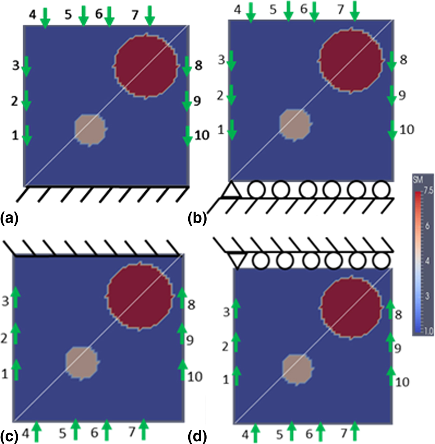
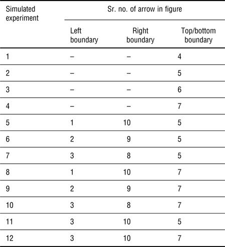
We consider a 1 cm × 1 cm domain with two stiff inclusions: a small inclusion with a radius of 0.1 cm and a larger one with a radius of 0.2 cm surrounded by a softer homogeneous background material as shown in Fig. 1. The coordinates of the center of the inclusions are (0.4 cm, 0.35 cm) and (0.75 cm, 0.75 cm) for the small and large inclusions, respectively, assuming that the coordinate system's origin (0 cm, 0 cm) is at the bottom left corner. The target shear modulus value of the background is 10 kPa and the shear moduli are 50 kPa for the small inclusion and 75 kPa for the large inclusion. As shown in Fig. 1(a), we have fixed the bottom boundary and forces represented by arrows are applied on top edge as well as on sides. The problem domain is discretized with 7200 linear triangular elements (61 nodes are uniformly distributed in each direction). The forces are applied only in vertical directions. Varying the locations of force application represents a new simulated experiment and provides distinct boundary displacement data sets, which ultimately will help in achieving well-recovered shear modulus distributions. Each arrow representing a force has been assigned a number and their combined loadings for each simulated experiment have been summarized in Table I. A total of 12 simulated experiments were conducted and will be used to solve the inverse problem later in this section. Further, in each simulated experiment, a force of 0.2 N is applied and distributed over eight finite element nodes. For example, for the simulated experiments 1–4 in Table I, the single force indentations are applied on the top boundary edge sequentially and each distributed over eight neighboring nodes. On the other hand, for simulated experiments 5–12 in Table I, the forces are applied as a combination of forces on sides as well as on top edges. In this scenario, the forces are distributed on four neighboring nodes at the top and two neighboring nodes on each left and right boundaries. This force will produce small deformations and can be effectively measured using digital cameras and displacement-tracking techniques discussed in the Introduction section. The resulting boundary displacements on all three edges are assumed to be the “measured” data. We also add 0.1% and 1% random noise to the boundary displacements, since measured data contain noise.
The problem domain with two stiff inclusions surrounded by a softer background material. Along the diagonal line, the shear modulus reconstructions are plotted and analyzed. The arrows indicate all applied forces and are combined according to Table I. (a) Fixed boundary conditions are applied on the bottom edge; (b) roller support conditions are imposed on bottom edge; (c) top boundary is subjected to fixed conditions; (d) top boundary is supported with rollers. Note: SM represents reconstructed shear modulus (unit in the color bar: 10 kPa).

Combination of forces applied on the boundaries.

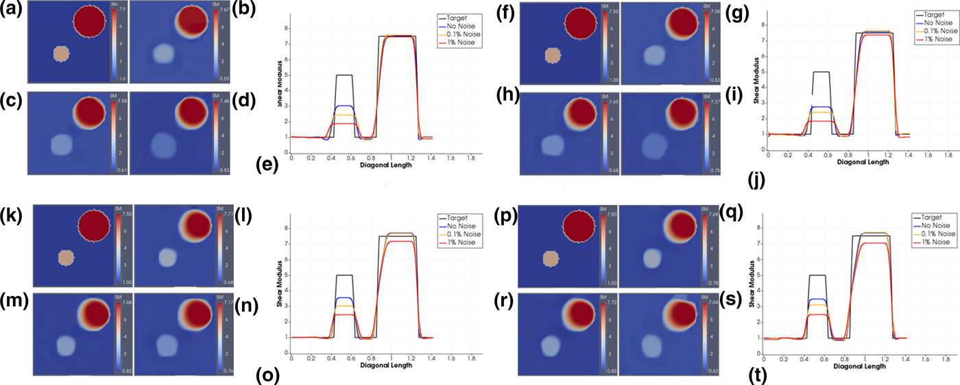
The reconstructed shear modulus distributions are given in Figs 2(b)–2(d) for noise levels of 0% (i.e., without noise), 0.1%, and 1%, respectively, together with the target shear modulus distribution in Fig. 2(a) for comparison. In Fig. 2(e), we plot the reconstructed shear modulus values along the diagonal line introduced in Fig. 1(a). The regularization factors for the reconstructions in Figs 2(b)–2(d) were chosen to be 1 × 10⁻¹³, 5 × 10⁻¹², and 1 × 10⁻¹⁰, respectively. We observe that the locations of the inclusion centers are identified precisely for all noise levels. However, we notice that the shear modulus value for the small inclusion has been significantly underestimated and its circular shape appears to increase in diameter with increasing noise levels. The large inclusion on the top right corner has been reconstructed very well and is close to the target inclusion for all noise levels.
(a) Target shear modulus distribution and (b)–(d) shear modulus reconstructions for 0%, 0.1%, and 1% noise levels for bottom boundary with fixed support [Fig. 1(a)], respectively. (f) Target shear modulus distribution and (g)–(i) shear modulus reconstructions for 0%, 0.1%, and 1% noise levels for bottom boundary with roller support [Fig. 1(b)], respectively. (j) Target shear modulus distribution and (l)–(n) shear modulus reconstructions for 0%, 0.1%, and 1% noise levels for top boundary fixed [Fig. 1(c)], respectively. (p) Target shear modulus distribution and (q)–(s) shear modulus reconstructions for 0%, 0.1%, and 1% noise levels for top boundary with roller support [Fig. 1(d)], respectively. (e), (j), (o), and (t) Shear modulus plot over diagonal line for reconstructed shear modulus with 0%, 0.1%, and 1% noise levels for bottom boundary with fixed support [Fig. 1(a)], bottom boundary with roller support [Fig. 1(b)], top boundary fixed [Fig. 1(c)], and top boundary with roller support [Fig. 1(d)]. Note: SM represents reconstructed shear modulus (unit in the color bar: 10 kPa).
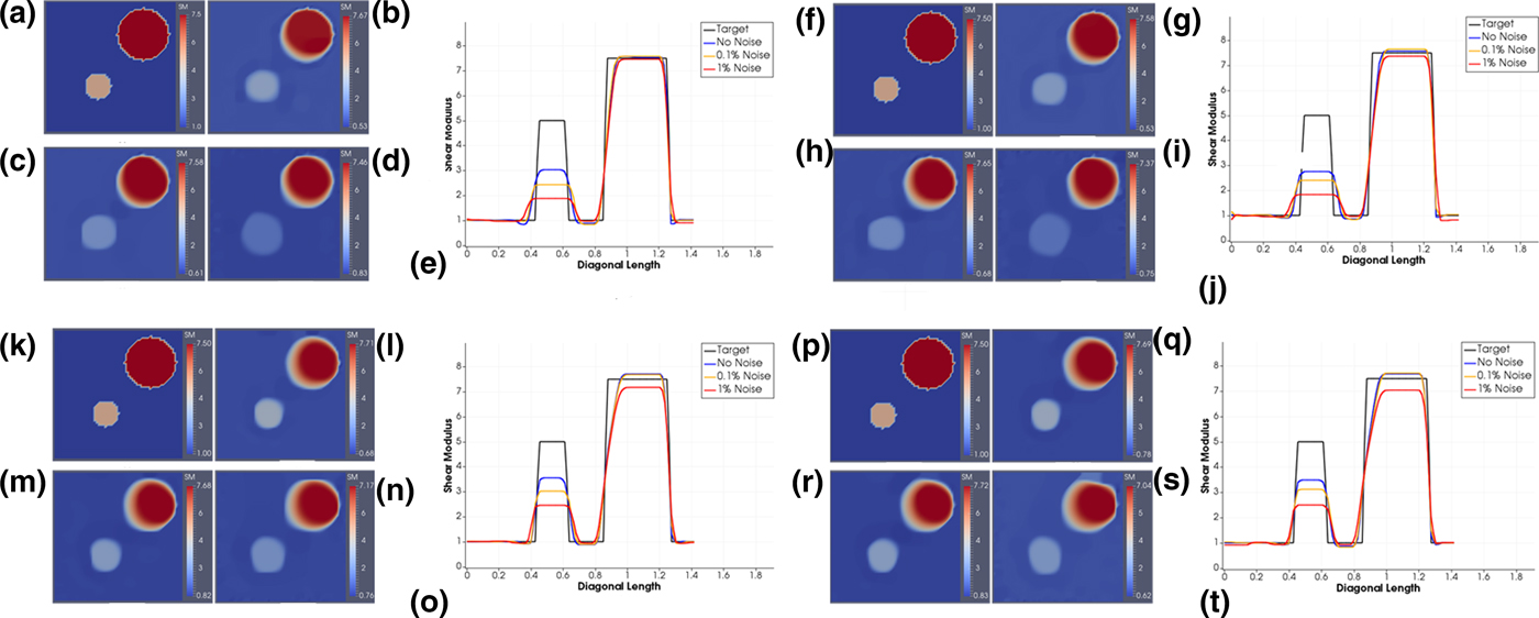
Figure 2(e) represents the shear modulus plots for all noise levels together with the target over the diagonal line drawn in Fig. 1(a). Conclusions stated above are clearly observed in this plot.
In Fig. 1(b), we have replaced the previous fixed support with a roller support. The applied forces and other parameters described for the previous problem remain the same. We select the regularization factors of 5 × 10⁻¹³, 5 × 10⁻¹², and 1 × 10⁻¹⁰ for 0%, 0.1%, and 1% noise levels, respectively. The shear modulus reconstructions for these noise levels are depicted in Figs 2(f)–2(j). We observe that the reconstructions are of similar quality to the case with fixed boundary conditions and exhibit similar trends.
In the previous examples, we observed that the small inclusion has been significantly underestimated in both problem domains, i.e., with roller and fixed support. For most in vitro samples, we can move and rotate the sample and with that change the location of supports. Thus, we will make use of this strategy to improve the contrast of the small inclusion. More precisely, we define the problem domain with fixed boundary conditions on the top edge, which could be interpreted as the original sample being rotated by 180°. The forces are applied to the bottom, left, and right boundary edges as shown in Fig. 1(c). A vertical force of 0.2 N is distributed over a total of eight finite element nodes as described earlier for the problem domain in Fig. 1 and the combination of applied forces for each simulated experiment (total of 12) is according to Table I. The shear modulus reconstructions are given in Figs 2(l)–2(n) for noise levels of 0%, 0.1%, and 1% and regularization factors of 5 × 10⁻¹³, 5 × 10⁻¹², and 1 × 10⁻¹⁰, respectively. Figure 2(k) represents the target shear modulus distribution for comparison. We also provide the shear modulus values along the diagonal line drawn in Fig. 1(c) for all noise levels together with the target in Fig. 2(o).
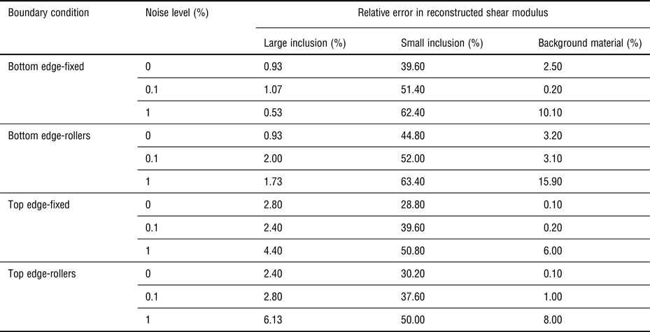
We notice that the reconstructions for all noise levels improved over the cases we discussed previously. The reconstructed shear modulus value for the small inclusion improved from 3.03 for the bottom fixed problem to 3.55 for the case with no noise in both problems. We also observe similar trends as in previous examples that with increasing noise level the recovered shear modulus value in the inclusion decreases and the inclusion diameter increases.
In the same fashion, keeping all the parameters same as in the previous example, we now support the top boundary with rollers as shown in Fig. 1(d) and apply forces as in the previous example according to Table I. The shear modulus reconstructions from these experimental simulations are shown in Figs 2(q)–2(s) for the noise levels of 0%, 0.1%, and 1% with regularization factors of 8 × 10⁻¹³, 5 × 10⁻¹², and 1 × 10⁻¹⁰, respectively. Figure 2(t) plots the reconstructed shear modulus values over the diagonal line depicted in Fig. 1(d). Overall, the shear modulus reconstructions are similar to the case with top boundary fixed conditions.
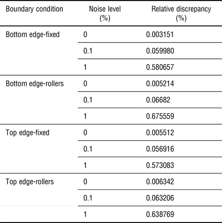
According to Morozov's discrepancy principal, the relative correlation between measured and computed displacements in Eq. (1) should be of the order of the noise level. To show that this is indeed the case, we calculate the relative discrepancy with the following formula:
 $$e = \sqrt {\displaystyle{{\sum\limits_{i = 1}^N {\left[ {\sum\limits_{e = 1}^{n_e} {\int\limits_{\Omega _e} {{\left( {{\bf N}_{}^e ({\bf x}){\left( {{\bf u}_e^i - {({\bf u}_e^i )}_{{\rm meas}}} \right)}_{}} \right)}^2d\Omega}}} \right]}} \over {\sum\limits_{i = 1}^N {\left[ {\sum\limits_{e = 1}^{n_e} {\int\limits_{\Omega _e} {{\left( {{\bf N}_{}^e ({\bf x}){({\bf u}_e^i )}_{{\rm meas}}} \right)}^2d\Omega}}} \right]}}}} \times 100\% $$
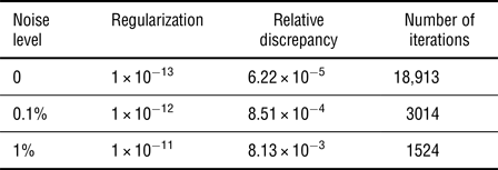
and summarize the calculations in Table II for all previous examples. We observe that the noise level differs by about a factor of 2 from the relative discrepancy for the noise levels of 0.1% and 1%, and is very small for the case with no noise.

We also calculate the error in the shear modulus reconstruction according to
 $$\; e = \sqrt {\displaystyle{{{\left( {\bar \mu - {\bar \mu} ^0} \right)}^2} \over {{\left( {{\bar \mu} ^0} \right)}^2}}} \times 100\% $$
where  $\bar \mu \; $ and
 $\bar \mu ^0$ are average recovered shear modulus and target shear modulus observed for a particular region of the domain, respectively (see Table III).
Relative error in shear modulus of inclusions and background.

Comparison of the shear modulus reconstruction with the target values is carried out for the stiff inclusions and the background material. For the average reconstructed shear modulus value of background material, the aberrations near the edge of the inclusions are neglected when calculating the error.
Two-dimensional problem domain with nine stiffness inclusions
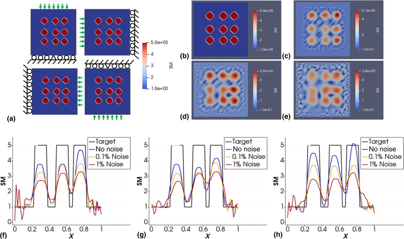
In this section, we consider a 1 cm × 1 cm domain with nine stiff inclusions of radii 0.07 cm shown in Fig. 3(a) with varying support locations. The vertical locations of the inclusion centers are at 0.3, 0.5, and 0.75 cm from the bottom edge, and the horizontal locations of the inclusion centers are at 0.3, 0.55, and 0.75 cm from the left edge. The shear modulus of all inclusions is 50 kPa, while the background has a shear modulus value of 10 kPa. The problem domain is discretized with 7200 linear triangular elements (61 nodes are uniformly distributed in each direction). Each indentation is applied in a separate simulated experiment with a total number of 28 simulated experiments. In each simulated experiment, nodal forces of 0.1 N are applied to three neighboring nodes. Thus, the total force applied in each simulated experiment is 0.3 N. Figures 3(c)–3(e) represent the shear modulus reconstructions for 0%, 0.1%, and 1% noise, respectively, together with the target problem domain in Fig. 3(b) as comparison. It is observed that with increasing noise level, the shear modulus values of the inclusions decrease and their shapes deteriorate. Figures 3(f)–3(h) is the reconstructed and target shear moduli over the horizontal lines passing through the center of the inclusions on different rows. Overall, the inclusions are well recovered.
(a) Seven indentations are applied on each side sequentially, while the opposite side is roller supported. The center node of the supported side is fixed to avoid rigid body motion. Distance between adjacent indentations is 0.1 cm. Each arrow represents a single indentation that is applied in a single simulated experiment (total of 28). (b) Target shear modulus distribution; (c) reconstruction with zero noise; (d) reconstruction with 0.1% noise; (e) reconstruction with 1% noise. Comparison of reconstructed and target shear moduli over the horizontal lines passing through the center of the inclusions (f) on the bottom row; (g) on the middle row; (h) on the top row (unit in the color bar: 10 kPa).
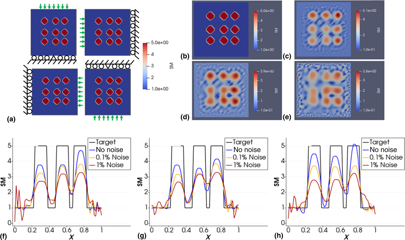
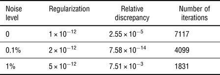
In Table IV, we report the regularization factors selected for each noise level and the relative discrepancy in the data fit defined in the “Methods” section. It is observed that the discrepancy is of the order of the noise level for 0.1% and 1% noise.
Regularization, relative discrepancy, and number of iterations for cases presented in Fig. 3.

Three-dimensional problem domain with one stiff inclusion
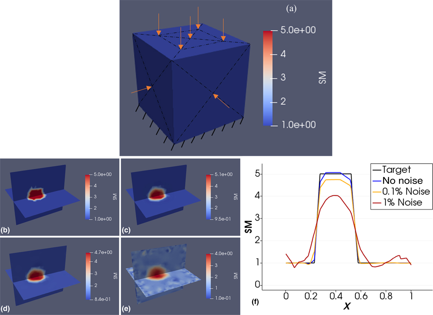
We define a cube with side lengths of 1 cm [see Fig. 4(a)] containing a stiff inclusion of radius 0.15 cm, with its center located at (0.4, 0.5, 0.5) cm measured from one corner. The shear modulus of the inclusion and background are 50 kPa and 10 kPa, respectively. The mesh is composed of 20,738 nodes and 108,567 linear tetrahedral elements. Each edge is discretized using 31 equally spaced nodes resulting in a structured mesh composed of 2 × 30 × 30 triangular elements on each surface. The mesh within the cube is unstructured though. Force indentations are applied sequentially at different locations with each indentation having a total force of 0.05 N and being distributed over five neighboring nodes. Four indentations are applied sequentially for each simulated experiment to the centers of the left, right, front, and back face. In Fig. 4(a), the arrows on the right and back sides are not visible. Five indentations are applied to the top as shown in the figure. Thus, a total of nine simulated experiments have been obtained and their surface displacements utilized to solve the inverse problem. Figures 4(c)–4(e) show the reconstructed shear modulus distribution for 0%, 0.1%, and 1% noise, respectively, together with the target problem domain in Fig. 4(b) as comparison. We observe that the inclusion has been very well recovered with respect to its shape and its shear modulus values for all noise levels. We also observe that the quality of the reconstructed solution deteriorates with increasing noise level. Figure 4(f) plots the shear modulus over the horizontal line passing along the intersection of the two planes shown in Fig. 4(a) and passing through the center of the inclusion.
(a) Boundary conditions. Each arrow represents a single indentation used for each simulated experiment (top subfigure). Shear modulus: (b) target distribution; (c) reconstruction with zero noise; (d) reconstruction with 0.1% noise; (e) reconstruction with 1% noise. Comparison of reconstructed and target shear moduli over the horizontal lines passing through the center of the inclusion along the intersection of the planes depicted in (f) (unit in the color bar: 10 kPa).
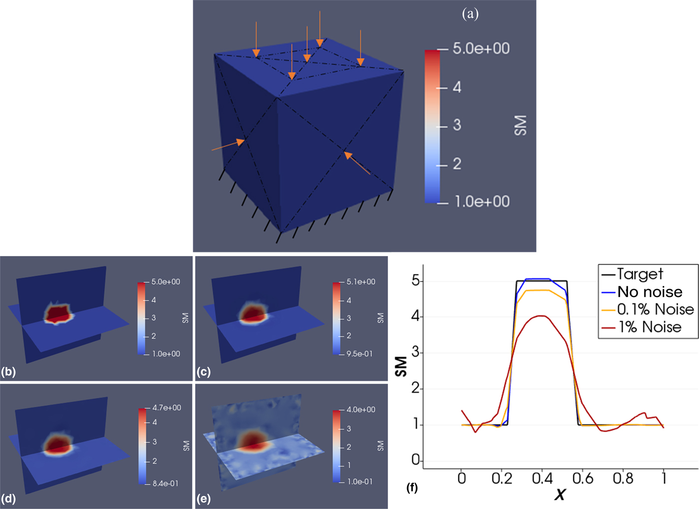
In Table V, we report the regularization factors selected for each noise level and the relative discrepancy in the data fit defined in the “Methods” section. It is observed that the discrepancy is in the order of the noise level for 0.1% and 1% noise.
Regularization, relative discrepancy, and number of iterations for cases presented in Fig. 4.

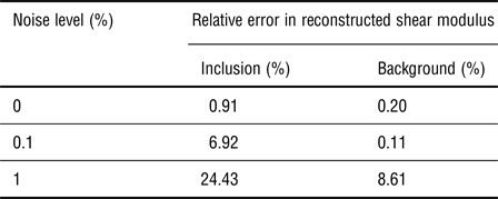
In Table VI, we report the relative error in the reconstructed shear moduli for inclusion and background with and without noise for several selected points within these regions. We observe that the error increases with the noise level with the exception of error in the background from no noise to 0.1% noise. This may be due to the fact that the error with 0.2% and 0.11% is quite low. We also report the computational time to be of the order of hours for the three-dimensional computations (about 8 h depending on how many iterations are needed).
Relative error in shear modulus for inclusion and background.

Discussion
In this paper, we analyzed the performance of solving the inverse problem in elasticity for the shear modulus distribution for two two-dimensional problem domains and a three-dimensional problem domain using solely boundary displacements that could be measured using digital camera techniques and known force applications. The two-dimensional problems were modeled as plane strain, thus displacements can only be measured on the boundary edges and not on the entire face, since these are not accessible for camera imaging. On the other hand, for plane stress problems, full-field displacements (i.e., displacements on the entire face) can be measured to solve the inverse problem with a rich data set. This was demonstrated in past studies by the authors with experimental data using a DIC system[Reference Mei, Stover, Kazerooni, Srinivasa, Hajhashemkhani, Hematiyan and Goenezen17] and simulated data.[Reference Mei, Tajderi and Goenezen18] Full field displacements yield a rich measurement data set that will facilitate to obtain a unique solution.
In this paper, we observe that it is feasible to solve the inverse problem in two-dimensional space for a plane strain problem using solely boundary displacement data. However, we do acknowledge that it is significantly harder than solving the inverse problem with full-field displacements. For the two-dimensional examples, we introduced one case with two inclusions having distinct stiffness values and diameters. We observed that the small inclusion being further away from the boundary edges was harder to recover than the larger inclusion being closer to the boundary edges. Furthermore, we realized that supports (roller and fixed) in proximity of the inclusions aggravates their reconstructions. The choice of support, roller or fixed, did not make a significant difference in the shear modulus reconstructions. Additionally, we presented the solution of the inverse problem in three dimensions, but utilized a coarse mesh with 20,738 nodes and 108,567 linear tetrahedral elements to reduce computational time overall. This implies that the three-dimensional problem consisted of 20,738 unknown shear moduli. Our inverse solution strategy successfully recovered the shear modulus distribution utilizing only nine boundary displacement data sets from simulated experiments.
We added white Gaussian random noise to the simulated boundary displacements to mimic actual displacement measurements, e.g., using digital cameras. The noise levels of 0.1% and 1% are significantly higher than the noise levels anticipated from actual displacement measurements using digital cameras and displacement-tracking programs. We observed that with increasing noise level, the shear modulus reconstructions deteriorated overall. In more detail, with increasing noise levels (1) the shear modulus values in the stiff inclusions and background decreased, (2) the inclusion shapes deteriorated, and (3) oscillations in the shear modulus distributions were more pronounced.
We acknowledge that utilizing white Gaussian noise may not fully represent noisy data from actual experimental measurements. In our earlier publication[Reference Mei, Stover, Kazerooni, Srinivasa, Hajhashemkhani, Hematiyan and Goenezen17] we have used a DIC system to measure full-field displacement data to solve the inverse problem for a problem domain having two inclusions of varying sizes. Therein, we also simulated data acquisition with finite element methods and added white Gaussian random noise to the simulated displacement measurements. We observed that the results from simulated experiments closely resembled the results using actual experimental measurements, thus the type of noise as well as the noise level seem to be a reasonable assumption. Nevertheless, future works will focus on a proof of concept using actual experimental data obtained via a DIC system.
The shear moduli in the inclusions were assumed to be 5 and 7.5 times stiffer than the background. As the stiffness ratio of inclusion to background becomes smaller and approaches 1, it is expected that the sensitivity of this method may not be sufficient to infer the shear modulus distribution accurately. On the other hand, if the stiffness ratio of inclusion to background is being increased and grows large, the inclusion will relatively behave like a rigid solid and sensitivity of displacement response may be compromised to infer the shear modulus distribution accurately. Additional factors that may affect the accuracy of the reconstructions are the total number of inclusions being modeled and the noise level. To explore the limitations of this inverse approach with respect to the discussion above, a large number of computations needs to be performed and is beyond the scope of this paper.
It is understood that most soft tissues as well as engineered soft tissue scaffolds have a pronounced non-linear mechanical response and non-linearity has not been modeled in this paper. The non-linear elastic response however is typically observed at large deformations; thus, given that the overall deformations are small, a linear elastic constitutive model may be sufficient to represent the mechanical response at small strains. We note that non-linear constitutive models can conveniently be implemented in the inverse problem formulation by changing the constraint of the optimization problem and modifying the adjoint equations accordingly. While it is anticipated that mapping the non-linear model parameters may be significantly harder to map with boundary displacement measurements and may also be more sensitive to measurement noise, we have not tested it at this point and will be part of our future studies.
Maybe more importantly than representing the non-linear mechanical behavior of the specimen would be to use the shear modulus distribution from the linear elastic model to delineate the morphology of soft tissues. For example, the morphology of the entire breast could potentially be mapped in vivo and non-invasively via the shear modulus reconstruction and could aid in visualizing tumors, lobes of the mammary gland, or ducts. It could also help to monitor the changes in extracellular matrix (ECM) of engineered tissues non-destructively, e.g., after seeding a hydrogel with cells. As these cells secrete collagen fibers, the structural integrity of the ECM changes and with that the shear modulus. These shear modulus distributions will significantly differ from the inclusion models in this paper and may in part need to be modeled as functionally graded materials. Since the shear moduli in the present inverse formulation are unknowns on finite element mesh nodes and interpolated with finite element shape functions, continuity of the shear modulus distribution in the problem domain is warranted and functionally graded materials representable. In this paper, the inclusions had abrupt changes at their interface and future works will include testing of this approach with functionally graded materials. Finally, we also acknowledge that our models do not take into account anisotropy and feasibility of mapping anisotropic elastic properties using boundary displacement measurements will be subject for future studies.
Conclusions
We presented for the first time the feasibility to recover the volumetric shear modulus distribution in three-dimensional space using surface displacements only. We recovered the shear modulus distribution of a stiff inclusion within a cubic softer background. Due to computational time constraints of three-dimensional problems, we analyzed the feasibility of more involved shear modulus distributions using two-dimensional problems. The results of this paper are encouraging and may open up new opportunities to characterize heterogeneous materials for their mechanical property distribution. We acknowledge that the experiments in this paper were simulated including high noise levels, and actual experimental data are needed to further analyze the potential of this approach.
Acknowledgments
The authors would like to acknowledge funding from the National Science Foundation under Grant No. CMMI #1663435 and thank for their support. The authors would also like to thank the High Performance Research Computing at Texas A&M University for their computing resources.