1. Introduction
Target tracking refers to tracking and identifying information such as the position, velocity, and state of a target within a continuous time series. In the field of robotics, target tracking is the foundation of many core tasks and is widely applied in key areas such as navigation, environmental perception, and path planning [Reference Sun, Zhao, Shi, Liu and Liu1–Reference Sharma and Voruganti3]. Especially in industries like logistics, security, and autonomous driving, it not only enhances the autonomy and intelligence of robotic systems but also drives technological advancements in these fields. Logistics delivery robots need to navigate in dynamic environments and accurately track the position of items or targets, particularly in open spaces or crowded scenarios, ensuring timely and accurate deliveries. In security monitoring, robots or drones utilize target-tracking technology to identify and track suspicious individuals or objects in real time, especially in large-area surveillance. This improves the efficiency of automated patrol systems, reduces labor costs, and enhances security response capabilities. In autonomous vehicles, target tracking helps the vehicle monitor the movement trajectories of other road users (such as pedestrians, other vehicles, bicycles, etc.) in real time. This enables the vehicle to make decisions on evasion or route adjustments, ensuring driving safety [Reference Wang, Jia, Lai and Shi4, Reference Gao, Ma, Zhang and Zhou5]. This process includes target recognition, localization, and path planning, often combining data from sensors such as vision systems, Light Detection and Ranging (LiDAR), and ultrasonic sensors, while utilizing computer vision, filtering algorithms (such as Kalman filters and particle filters), and deep learning techniques for target detection and tracking [Reference Tian, Liu, Zhang, Zheng and Dong6–Reference Liu, Yan, Wan, Li, Al-Rubaye, Al-Dulaimi and Quan8]. The challenges of target tracking include issues like occlusion, motion uncertainty, sensor noise, and environmental changes.
In the field of target recognition, deep learning-based methods have gained widespread acceptance due to significant improvements in detection accuracy [Reference Dong and Zhang9]. Unlike traditional approaches reliant on manually crafted features, deep learning models can directly learn powerful features from facial images [Reference Pan, Peng, Li, Han and Wang10, Reference Yadav, Nagar and Shah11]. These methods are typically categorized into single-stage and multi-stage frameworks, with single-stage models gaining attention for their computational simplicity and operational efficiency in recent years [Reference Liu, An, Chen and Zhao12, Reference Yang, Xu, Liu and Li13]. Cao et al. [Reference Cao, Wang, Li and Mao14] addressed the issue of small target omission or mis-detection in drone detection processes by proposing an improved YOLOv5s-based algorithm named YOLOv5s_MSES. Compared to existing methods, experimental results on the VisDrone2019 drone object detection dataset demonstrate that YOLOv5s_MSES achieves better detection performance, effectively completing small target detection tasks in drone aerial images. Xiong et al. [Reference Xiong, He, Li, Zheng, Xu, Fan and Zhang15] proposed the AS-YOLOV5 algorithm for small target detection by addressing the challenges posed by the complexity and variability of real-world road environments. This algorithm integrates adaptive feature fusion and improved attention mechanisms. During the feature extraction stage, AS-YOLOV5 employs soft pooling to enhance feature extraction networks, thereby mitigating the inherent loss of critical edge information of small targets in standard downsampling techniques. Chen et al. [Reference Chen, Wu, Peng, Li and Shang16] proposed a novel object detector based on continuous unsupervised domain adaptation to address the challenges of high scene complexity, small-scale targets, and model domain shift. This approach enhances the detection accuracy and generalization capability of the detector for small floating targets. However, many existing deep learning models prioritize higher accuracy, resulting in increasingly complex and parameter-heavy neural network structures, sometimes spanning hundreds or thousands of megabytes. This poses challenges for deployment on mobile or embedded devices with limited computational power and storage resources.
Research on target tracking control for mobile robots primarily focuses on identifying targets in the environment and directing the robot to track them. Currently, the main methods used are LIDAR-based and vision-based tracking control [Reference Wu, Tao, Wu, Gong and Yin17, Reference Pan, Li, Deng and Wei18]. Yan et al. [Reference Yan, Huang, Yang, Hasegawa and Fukuda19] proposed a walking aid robot for assisting patients in rehabilitation training, where they employed onboard laser range finder sensors to track human users. However, these sensors somewhat hinder tracking performance as they do not easily discern human direction and intention. In contrast, Chen et al. [Reference Chen, Sahdev and Tsotsos20] utilized an online real-time convolutional neural network target tracker with a stereo camera to track and control human targets. Yet, this method is vulnerable to light variations and occlusions, affecting its tracking efficacy. LIDAR-based tracking is straightforward and less affected by lighting changes, but it solely provides distance information, limiting its adaptability to complex targets and environments [Reference Tai, Ilias, Shukor, Abdul Rahim and Markom21]. Vision-based tracking can capture more detailed target and environmental data but is sensitive to lighting changes, target deformations, and is constrained by the camera’s field of view, increasing the risk of losing track of the target [Reference Wang, Liu, Su, Liao, Shi and Miro22]. Each sensor type possesses distinct strengths and weaknesses in target tracking. Hence, exploring the integration of multiple sensors could leverage their respective advantages to enhance tracking performance. Thus, investigating multi-sensor combination approaches holds significant promise for advancing the technology of mobile robots in achieving robust target-tracking control.
The computing power of the control system carried by mobile robots is relatively low, which makes deploying intelligent algorithms challenging. To address the issue of insufficient computing power, a target tracking control algorithm based on lightweight networks is proposed in the paper. First, to accurately extract features, a feature extraction model based on a depthwise separable convolution backbone network is constructed. Then, an efficient channel attention module (ECAM) is introduced into the target recognition algorithm to reduce the impact of redundant features and focus on significant channels, thereby simplifying model complexity and improving network efficiency. Finally, a model predictive control (MPC) tracking strategy that integrates information from visual and ultrasonic sensors is proposed to achieve target following. Validation of the proposed algorithm is conducted using a mobile robot equipped with Raspberry Pi 4B. Experimental results demonstrate that the proposed algorithm achieves rapid target tracking.
The remainder of the paper is organized as follows: Section 2 outlines the lightweight recognition method and the employed target tracking strategy; Section 3 covers the experimental aspects, including demonstrations of the effectiveness and analysis of results from target detection comparison experiments and target tracking control experiments; Section 4 presents the conclusions drawn from this study and suggests future research directions.
2. Tracking control algorithm based on lightweight network
2.1. Lightweight recognition method
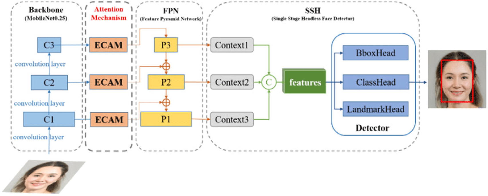
The target recognition method presents lightweight improvements to RetinaFace, as depicted in Figure 1. This method focuses on two main enhancements: (1) In the backbone network, depthwise separable convolutions are used to replace standard convolutions, significantly reducing computational parameters and improving interpretability; (2) The algorithm introduces ECAM, which selectively emphasizes the key channels for object detection, minimizing the impact of redundant features, thereby effectively reducing network complexity while improving efficiency. In addition, in terms of the loss function, the CIoU Loss (Complete Intersection over Union Loss) is used as the target bounding box regression loss to address the issue that the Smooth L1 loss is not equivalent to the actual evaluation metric IoU, while also improving the model’s validation accuracy.
Network architecture of improved RetinaFace.

To accommodate the neural network’s input size requirements and enhance feature extraction performance, preprocessing of input images is essential [Reference Cui, Li, Qu, Fan and Lu23]. Initially, the image is scaled from 320 × 240 to 320 × 320 to align with the model’s input size specified in this paper. Following scaling, mean subtraction is applied, which involves subtracting the mean pixel value of each channel from the corresponding pixels. This process improves the model’s capability to mitigate brightness variations in input images, thereby reducing the impact of illumination on target detection performance.
2.1.1 Lightweight backbone network
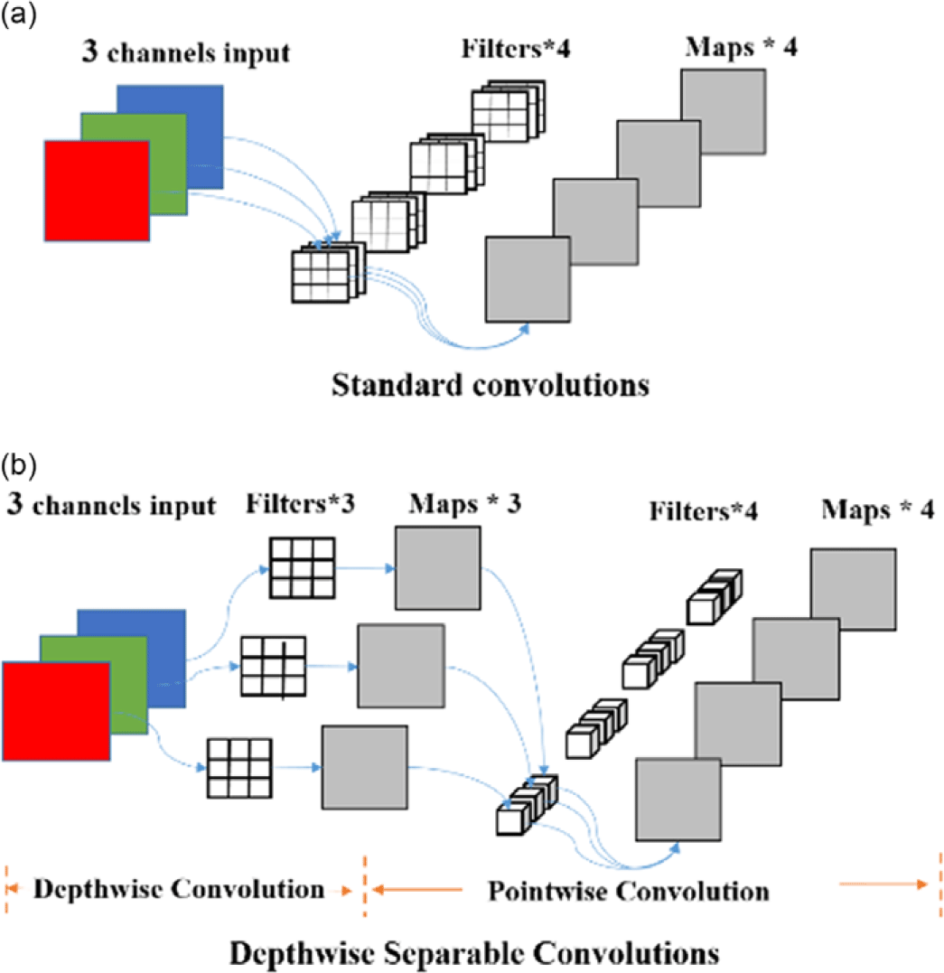
For mobile and embedded vision applications, MobileNet stands out as an excellent choice due to its lightweight architecture [Reference Biswas and Barma24]. In this study, we utilize MobileNet0.25, which employs depthwise separable convolutions as the backbone network. Figure 2 illustrates a comparison between depthwise separable convolution and standard convolution methods.
Standard convolutions and depthwise separable convolutions.

As depicted in Figure 2, depthwise separable convolution achieves equivalent feature map output size as standard convolution by decomposing it into depthwise convolution and pointwise convolution. Standard convolution extracts feature correlations within the image feature map and between channels, involving numerous parameters and posing interpretability challenges. In contrast, depthwise separable convolution divides these tasks, decreasing parameter count and enhancing interpretability. Thus, depthwise separable convolution markedly reduces computational parameters compared to standard convolution.
2.1.2 Efficient channel attention module
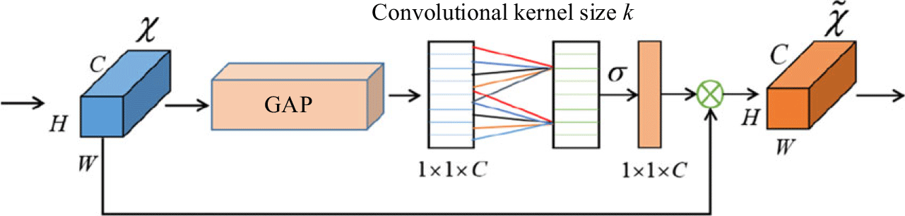
The ECAM is introduced to enhance the RetinaFace method. This module enables the network to diminish the impact of redundant features and prioritize channels crucial for target detection, thereby reducing model complexity and enhancing network efficiency. The structure of ECAM is illustrated in Figure 3.
Efficient channel attention module.

As illustrated in Figure 3, ECAM chooses average pooling to extract global information from each channel. It then utilizes a fully connected layer to learn channel weights, which are normalized using an activation function – a sigmoid function, as shown in Eq. (1). The kernel size(k) of the convolutional layer in the channel attention module depends on the number of channels, as depicted in Eq. (2). Where
 $| x| _{\mathrm{odd}}$
indicates the nearest odd number of
 $x$
.
 \begin{equation} \textit{sigmoid}\left(x\right)=\frac{1}{1+exp\left(-x\right)} \end{equation}
 \begin{equation} k=\left| \frac{\log _{2}C+1}{2}\right| _{\mathrm{odd}} \end{equation}
Following the feature extraction by ECAM, the target detection model incorporates a feature enhancement module to maximize the utilization of these extracted features, thereby significantly enhancing target detection accuracy. This enhancement is achieved through two primary modules: the Feature Pyramid Network [Reference Liu, Ning, Ma and Lian25] and the Single Stage Head-less network [Reference Zhang, Guo, He, Wang, Guo and Ding26], which are utilized for advanced feature extraction and further accuracy improvement in target detection.
2.1.3 Loss function
The loss function used for training the target detection model in this paper is shown in Eq. (3).
 \begin{equation} L=\lambda _{1}L_{cls\left({p_{i}},p_{i}^{*}\right)}+\lambda _{2}p_{i}^{*}L_{box}\left(t_{i},t_{i}^{*}\right)+\lambda _{3}p_{i}^{*}L_{pts}\left(l_{i},l_{i}^{*}\right) \end{equation}
The loss function consists of three main items,
 $L_{cls({p_{i}},p_{i}^{*})}$
is target classification loss,
 $L_{box}(t_{i},t_{i}^{*})$
is target frame regression loss, and
 $L_{pts}(l_{i},l_{i}^{*})$
is target information regression loss. According to the above task needs, in this paper, the loss-balancing parameters
 $\lambda _{1}, \lambda _{2}$
, and
 $\lambda _{3}\,$
are set 1, 2, and 0.1 respectively.
2.1.4 Lightweight deployment
Target detection models are deployed on embedded devices, where choosing the right inference computation framework is crucial for enhancing model efficiency. In order to further boost real-time performance of the target detection model on Raspberry Pi, refs. [Reference Qasaimeh, Denolf, Khodamoradi, Blott, Lo, Halder, Vissers, Zambreno and Jones27, Reference Putra and Imelda28] led to the selection of OpenCV’s DNN module for deployment and execution of the model. To deploy the target detection model, the trained model file is first converted to the ONNX format. Subsequently, installation of the relevant framework dependencies enables deployment. Once deployed, this approach enables the creation of a lightweight real-time target detection system on Raspberry Pi.
2.2 Target tracking control based on multi-sensor information
Target tracking relies primarily on two key pieces of information: target direction and distance. In traditional tracking methods using a single visual sensor, target direction information can be swiftly obtained, but accurately gauging distance is challenging. Typically, distance between the robot and the tracked target is roughly estimated based on the size of the detection frame area, leading to significant estimation errors and inadequate tracking performance in the target of target motion. Addressing these limitations, this paper proposes a target tracking method based on multi-sensor information. By integrating an ultrasonic sensor, accurate distance information of the target is obtained [Reference Zhu, Shi, Wang, Xue, Liao, Xiong, Kuang and Zhang29]. The direction information of the target is obtained through visual sensor data. The mobile robot uses the visual and distance information to implement target tracking using the PID control method.
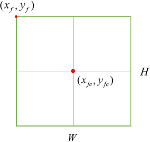
The pivotal aspect of the target tracking process in this paper involves processing the coordinates of the detected target frame, which are subsequently utilized as input for tracking control. The result of target detection returns the coordinates
 $(x_{f},y_{f})$
of the upper-left corner of the target frame and the width
 $W$
and height
 $H\,$
of the target frame, as shown in Figure 4.
Information of target detection frame.

According to the needs of tracking control input, the coordinates of the center of the target frame
 $(x_{fc},y_{fc})$
need to be calculated, and the calculation formulas are shown in Eqs. (4) and (5).
 \begin{equation} x_{fc}=x_{f}+\left(W/2\right) \end{equation}
 \begin{equation} y_{fc}=y_{f}+\left(H/2\right) \end{equation}
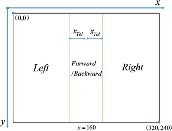
Target tracking control is primarily divided into left-right direction control and forward-backward distance control. The main objective of left-right direction control is to maintain the detected target frame within the central region of the video frame captured by the camera. The schematic diagram illustrating the left-right direction control for target tracking is depicted in Figure 5.
Control schematic of target tracking.

According to Figure 5, this is achieved by pre-setting a suitable directional threshold
 $X_{Tol}$
, which is relative to the width of the detection window and ranges between 0 and 1. Then the deviation
 $X_{Dev}$
between the center of the target frame and the center of the video frame in the X-coordinate direction is calculated, and the formula for the deviation
 $X_{Dev}$
is shown in Eq. (6).
 \begin{equation} X_{Dev}=\left(x_{fc}/W\right)-0.5 \end{equation}
The left-right tracking motion of the robot is controlled by comparing whether the deviation
 $X_{Dev}$
is within the threshold
 $X_{Tol}$
. The control command for left-right direction tracking is
 $C_{\mathrm{dir}\textit{ection}}$
, shown in Eq. (7).
 \begin{equation} C_{\textit{direction}}=\left\{\begin{array}{ll} \quad \quad \quad \quad turn\quad left & {\rm if}\quad X_{Dev}\leq -X_{Tol}\\ move\quad \textit{forward}/\textit{backward} & {\rm if}\quad \left| X_{Dev}\right| \lt X_{Tol}\\ \quad \quad \quad \quad turn\quad \textit{right} & {\rm if}\quad X_{Dev}\geq X_{Tol} \end{array}\right. \end{equation}
It is worth mentioning that the control output in the left-right direction is based on the action time input to the motor, which is adjusted by the magnitude of the deviation
 $d_{\textit{direction}}$
. The calculation formula of
 $d_{\textit{direction}}$
is shown in Eq. (8).
 \begin{equation} d_{\textit{direction}}=\left| X_{dev}\right| -X_{Tol} \end{equation}
In general, the larger the value of the deviation
 $d_{\textit{direction}}$
, the larger the output motor action time
 $t_{\textit{direction}}$
, and vice versa. There is a linear relationship between
 $t_{\textit{direction}}$
and
 $d_{\textit{direction}}$
with a coefficient
 $k$
, which is determined according to the actual situation, the formula is shown in Eq. (9).
 \begin{equation} t_{\textit{direction}}=k\times d_{\textit{direction}} \end{equation}
The forward-backward distance control of target tracking is to make the mobile robot always keep a suitable and safe distance from the target in the process of target tracking, so as to achieve a safe and effective tracking effect. The prerequisite for the forward-backward distance control is that
 $| X_{Dev}|$
is less than
 $X_{Tol}$
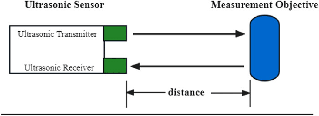
after the mobile robot has completed the current direction control. The hardware basis for distance control of target tracking is an ultrasonic sensor. The principle of distance measurement by ultrasonic sensors is shown in Figure 6.
Ultrasonic sensor distance measurement.

As in Figure 6 the ultrasonic sensor has an ultrasonic transmitter and an ultrasonic receiver. The distance between the ultrasonic sensor and the target can be measured by recording each ultrasonic emission moment
 $t_{\textit{transmitter}}$
and ultrasonic reception moment
 $t_{\textit{receiver}}$
combined with the acoustic velocity
 $v$
The formula for calculating the measurement distance
 $d$
is shown in Eq. (10).
 \begin{equation} d=\left[\left(t_{\textit{receiver}}-t_{\textit{transmitter}}\right)\times v\right]/2 \end{equation}
A suitable safety distance
 $(D_{\min },\,D_{\max })$
is predetermined, and then the distance
 $d$
between the mobile robot and the measured target is measured with the help of ultrasonic sensors. The forward-backward distance control of the mobile robot is performed by comparing
 $d$
with
 $(D_{\min },\,D_{\max })$
. The control command for forward-backward distance tracking is
 $C_{\textit{distance}}$
, and the calculation formula is shown in Eq. (11).
 \begin{equation} C_{\textit{distance}}=\left\{\begin{array}{ll} move\quad \textit{forward} & {\rm if}\quad d\gt D_{\max}\\ \quad \quad stop & {\rm if}\quad D_{\min}\leq d\leq D_{\max}\\ move\quad \textit{backward} & {\rm if}\quad d\lt D_{\min} \end{array}\right. \end{equation}
It should be noted that the forward-backward distance control of target tracking is implemented on the basis of
 $| X_{dev}| \leq X_{Tol}$
.
This paper aims to implement a trajectory-tracking controller through MPC, with the core objective of achieving high-precision trajectory-tracking control by using control inputs with minimal and smooth variations. Specifically, this means that at each moment, the robot’s state
 $\xi$
should be able to accurately track the reference state
 $\xi _{r}$
. Meanwhile, the robot’s input control
 $u$
should remain as close as possible to the reference control
 $u_{r}$
while maintaining minimal variation, subject to system constraints. Based on the above analysis of the MPC strategy, the optimization objective function in the rolling optimization process can be formulated as a function of the robot’s state
 $\xi$
and input control
 $u$
, as shown in Eq. (12):
 \begin{equation}\left(\xi, u\right)=\left\| \xi -\xi _{r}\right\| _{Q}^{2}+\left\| u-u_{r}\right\| _{R}^{2} \end{equation}
where
 $Q$
and
 $R$
represent the weight matrices, which are typically semi-positive definite matrices (
 $Q\geq 0, R\geq 0$
), and are adjusted to change the weight coefficients of different state and control terms according to specific needs. Specifically,
 $Q$
is used to weight the state tracking errors. By properly setting the elements in
 $Q$
, the importance of specific state variables can be emphasized or reduced, thereby achieving differentiated control of different state variables. Similarly,
 $R$
is used to penalize the variations in control inputs. By adjusting the weight coefficients in
 $R$
, the smoothness and magnitude of the control inputs can be controlled to prevent excessive control actions from having a negative impact on the system. By solving for the minimum value of the optimization objective function shown in Eq. (12), a series of optimal control sequences are obtained, as shown in Eq. (13):
 \begin{equation} u^{*}={\rm arg\,min}_{u}\left\{{\unicode[Arial]{x03A6}} \left(\xi, u\right)\right\} \end{equation}
The optimization process of MPC can be expressed as follows: at each sampling time
 $k$
, the controller based on the current robot state information and constraint conditions, along with the optimization objective function, solves the optimization problem to obtain an optimal control sequence
 $u^{*}=\{u(k|k),\ldots, u(k+N_{p}-1|k)\}$
and the corresponding minimum objective function cost
 $^{*}(\xi, u)$
.
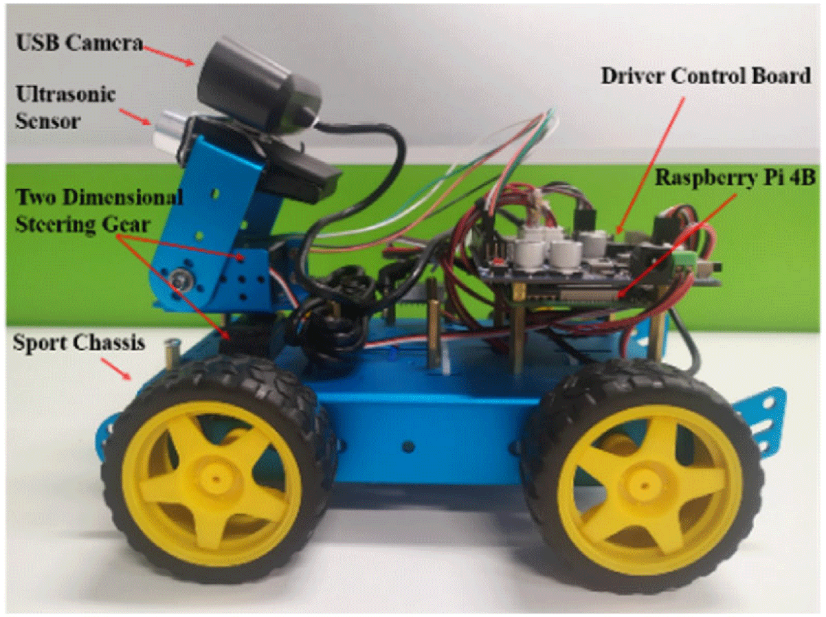
Experimental platform: differential wheel mobile robot based on Raspberry Pi 4B.

3. Experiment and analysis
3.1 Experimental platform
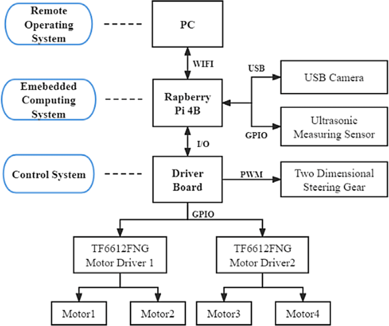
In this paper, a differential wheeled mobile robot based on Raspberry Pi 4B serves as the experimental platform, as illustrated in Figure 7. The hardware system of the experimental platform in this paper is designed with three layers: the control system, the embedded computing system, and the remote operating system. The architecture of the hardware system design is depicted in Figure 8. These three layers communicate and collaborate to achieve the functions of target detection and tracking control. The experiment aims to recognize faces and load the mentioned algorithm onto a Raspberry Pi-based mobile robot. The robot’s facial tracking performance is then validated in a laboratory environment without obstacles.
Robot hardware system architecture.

The lower control system primarily includes a drive board, motor driver, motor, and two-dimensional servo head. It is responsible for controlling the chassis motion and the servo head angle. The upper embedded computing system consists mainly of a Raspberry Pi 4B, USB camera, and ultrasonic sensor. Its main function is to execute visual perception algorithms and target-ranging modules. The remote operation system function is primarily managed by a mobile PC terminal. This layer monitors and oversees the operational functions of each part of the mobile robot.
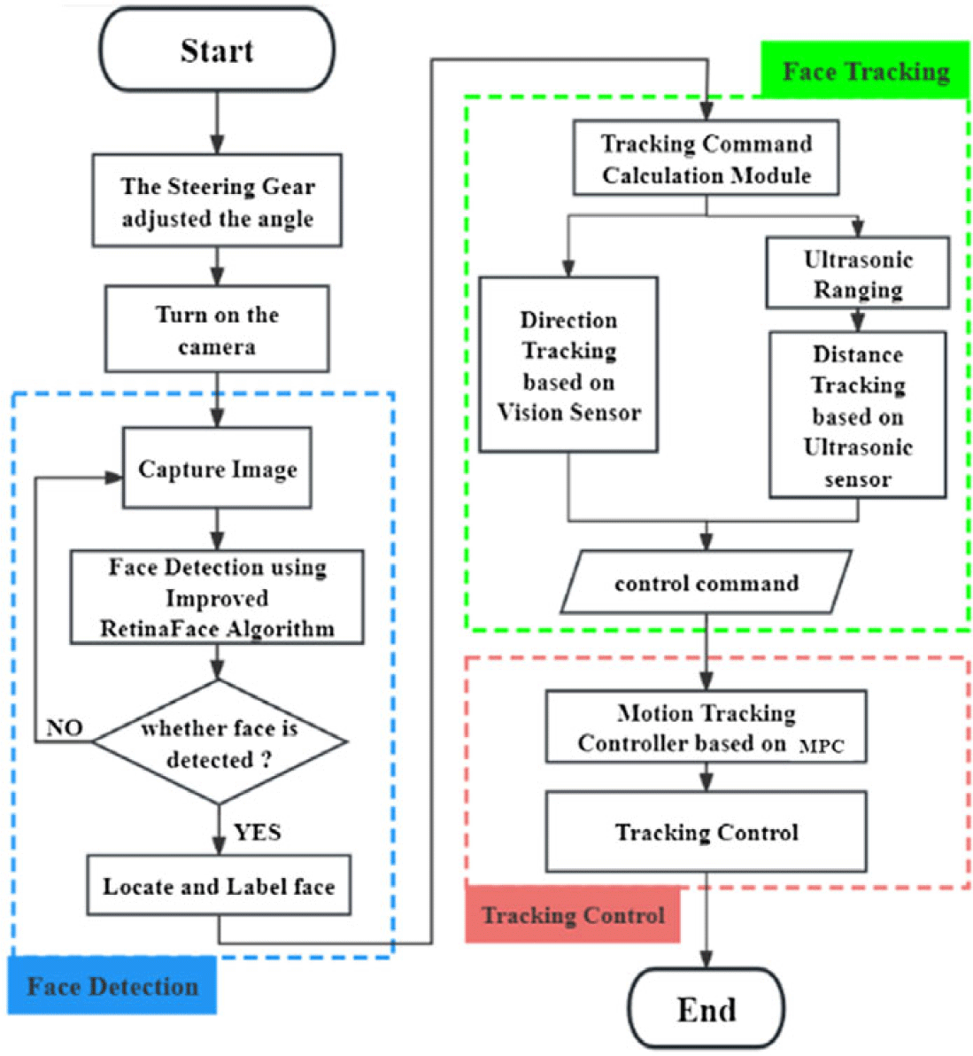
In this paper, faces are used as targets in the object-tracking experiments. The target detection and tracking control system proposed in this paper consists of three main modules: (1) a face detection module based on an efficient lightweight network; (2) a tracking decision module based on multi-sensor combination; and (3) a motion control module utilizing an MPC controller. The system flowchart is illustrated in Figure 9.
Face detection and tracking system flow.

As depicted in Figure 9, the process begins with the visual sensor gathering environmental data, employing an efficient and lightweight method based on enhanced RetinaFace for face detection, while an ultrasonic sensor measures the distance to the target face. Next, the face information and distance data are fed into the multi-sensor combination-based face tracking module, which calculates and outputs the appropriate tracking control commands. Finally, these commands are inputted into the motion control module, utilizing an MPC controller to achieve precise motion tracking of the detected face.
3.2. Target recognition experiment
3.2.1. Data set
In this paper, the WIDER FACE [Reference Yang, Luo, Loy and Tang30] dataset is used to train and test the face detection algorithm. The WIDER FACE dataset comprises 32,203 images with 393,703 annotated faces across 60 event categories. Each event category includes subsets categorized into three detection difficulty levels: Easy, Medium, and Hard. This categorization enables a detailed and nuanced evaluation of face detection performance. According to the official WIDER FACE dataset standards, the images are divided into training, validation, and test sets in a ratio of 4:1:5.
3.2.2. Evaluation indicators
In the context of face tracking control experiments on a Raspberry Pi using a deployed face detection model, two key metrics, AP (Average Precision) and
 $fps$
(frames per second), are employed to evaluate the model’s performance. AP measures the average accuracy rate, indicating the proportion of successfully identified samples among all recognized samples (N) (as depicted in Eq. (16)). Additionally, AP corresponds to the area under the Precision-Recall (P-R) curve, serving as an evaluation metric for face detection accuracy. Here, Precision (P) refers to the proportion of images with correctly detected faces out of all images with detected faces, and Recall (R) indicates the proportion of images correctly detecting faces out of all images containing faces. The formulas for calculating P and R are provided in Eqs. (14) and (15), respectively.
 \begin{equation} \textit{Precision}=\frac{TP}{TP+FP} \end{equation}
 \begin{equation} \textit{Recall}=\frac{TP}{TP+FN} \end{equation}
 \begin{equation} AP=\frac{1}{N}\sum _{i=1}^{m}\left(P\mathrm{re}\textit{cisio}n_{i}\right) \end{equation}
Typically, fps is generally used as an important indicator of detection speed. fps is the number of frames per second, which is how many images are processed per second. The units of fps are
 $f\cdot s^{-1}$
, and
 $f$
represents the number of frames processed. Higher fps means faster detection and better real-time performance.
Performance comparison of different face recognition models.

3.2.3. Experimental results and analysis
Firstly, the proposed face detection method RetinaFace (MobileNet0.25) + ECAM was evaluated using the WIDER FACE validation dataset, comparing its detection accuracy with RetinaFace [Reference Zhu, Ma, Xia and Zhou31, Reference Luo, Liu, Lin and Wang32] and LFFD [Reference Zhu, Shi, Wang, Xue, Liao, Xiong, Kuang and Zhang29] methods. Secondly, models trained based on these methods were quantized to measure their model size. Finally, these models were deployed on a Raspberry Pi 4B using a lightweight deployment method (refer to Section 2.1.4 for details) to compare their detection speeds. Compare the performance of these methods in terms of AP, model size, and detection speed on Raspberry Pi 4B, as shown in Table I.
Table I illustrates that the face detection method introduced in this paper exhibits superior overall performance and broader applicability. While the proposed method does not match RetinaFace (ResNet50) in detection accuracy, its lightweight backbone network based on depthwise separable convolution significantly reduces network parameters and model size. This reduction enhances its suitability for real-time face-tracking tasks. Furthermore, compared to RetinaFace (MobileNet0.25), the proposed method incorporates an attention mechanism to boost network efficiency, resulting in notable accuracy improvements. Specifically, average accuracies on the easy, medium, and hard datasets of the WIDER FACE validation partition increased by 1.2%, 1.4%, and 1.1%, respectively. Overall, the proposed method achieves a balanced blend of detection accuracy and speed, making it highly suitable for embedded applications. This capability is crucial for deploying face detection systems on low-performance embedded devices.
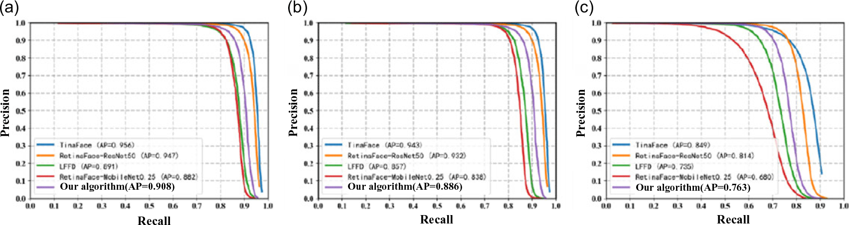
To provide a more intuitive comparison of the accuracy between the proposed algorithm and other algorithms, the target recognition results of the proposed algorithm and other algorithms on the three validation subsets of WIDER FACE are shown using P-R curves, as illustrated in Figure 10.
Results of model ablation experiments.

P-R curves of several face detection algorithms on the WIDER FACE validation set (a) Easy set (b) Medium set (c) Hard set.

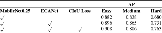
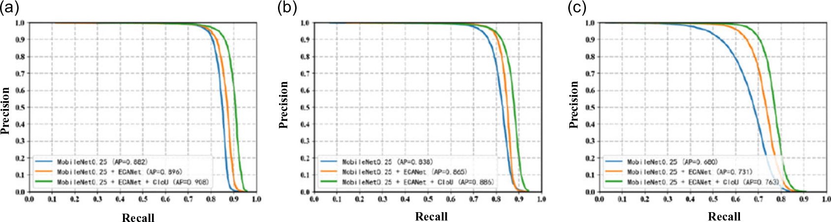
To further test the performance of the mentioned algorithm, this paper conducts ablation experiments based on the RetinaFace network architecture, using MobileNet0.25 as the backbone for feature extraction. The experiments verify the effectiveness of the efficient channel attention module ECANet and the improved loss function CIoU Loss. The experimental data are shown in Table II. The ablation experiment P-R curve on the WIDER FACE validation set is shown in Figure 11.
From the data in Table II, it can be seen that after using the MobileNet0.25 lightweight network as the feature extraction backbone, the model’s average precision on the three difficulty validation subsets of WIDER FACE are 0.882, 0.838, and 0.680, respectively. Compared to face detection models with heavyweight backbone networks, its detection accuracy has not yet reached the expected performance in practical application scenarios. After introducing the efficient channel attention module ECANet after the backbone network, the model’s detection accuracy on the three difficulty validation subsets of WIDER FACE improved by 1.4%, 2.7%, and 5.1%, respectively. The experimental results demonstrate that the proposed ECANet module significantly enhances face detection accuracy, particularly in terms of improving the detection accuracy of complex faces in the challenging subsets. This improvement is due to the integration of the attention mechanism, which enables the network to focus more on the important channel features for face detection. By optimizing the face bounding box loss function with CIoU Loss, the proposed method achieved improvements in average precision of 1.2%, 2.1%, and 3.2% on the three difficulty validation subsets of WIDER FACE, demonstrating the effectiveness of CIoU Loss in enhancing face localization accuracy and detection rate. Overall, the proposed model, based on improvements to the RetinaFace network architecture, achieved average precision increases of 2.6%, 4.8%, and 8.3% on the three difficulty validation subsets of WIDER FACE. Therefore, the experimental results fully validate the effectiveness of the proposed improvement module based on the RetinaFace network in enhancing face detection performance.
3.3. Target tracking control simulation and experiment
3.3.1. Target tracking control simulation
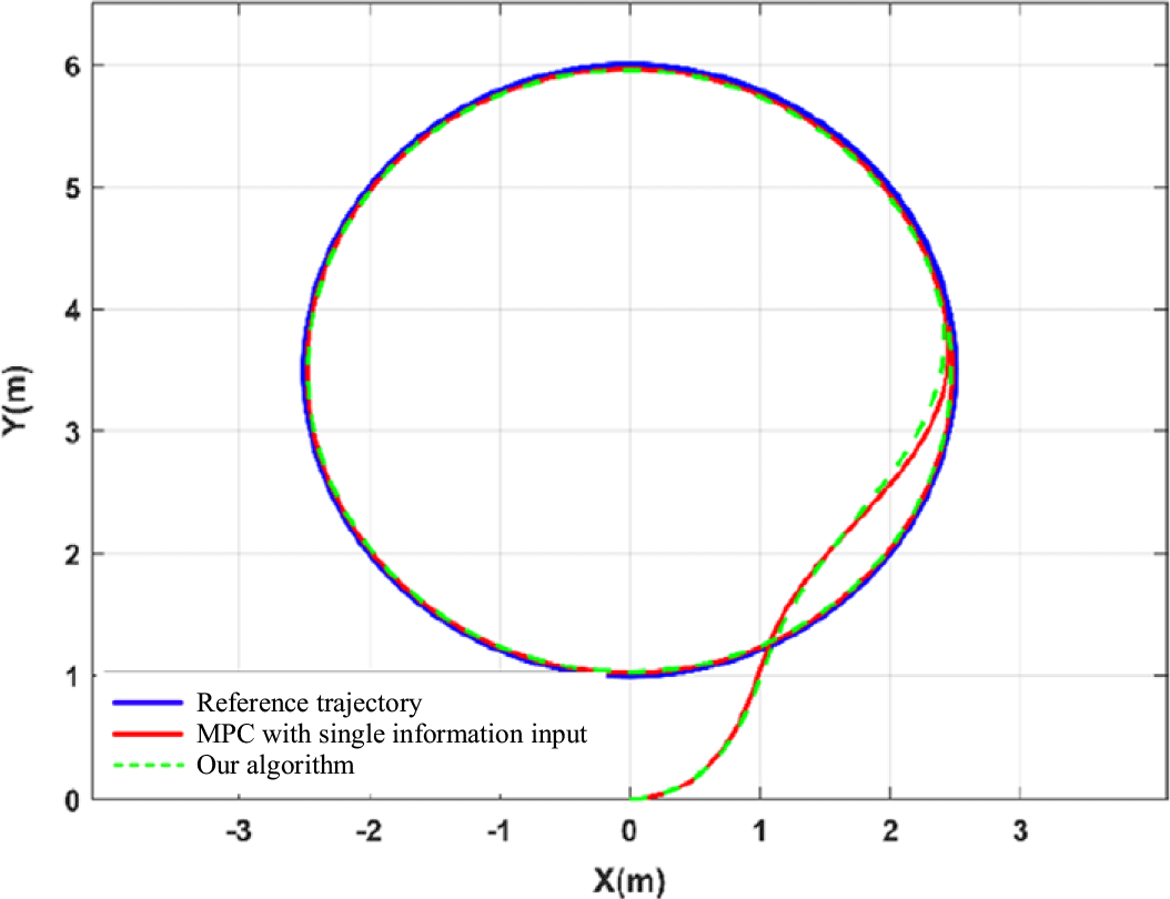
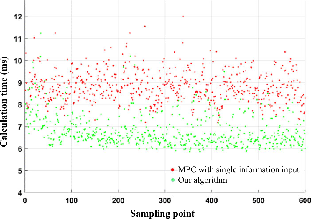
The target direction and distance information are simultaneously input into the MPC control function for circular trajectory tracking simulation. The tracking performance is compared with the MPC method that only uses direction information as input under the same experimental conditions. The trajectory tracking results are shown in Figure 12, while the comparison of the controller’s computation time for all time steps during the tracking process is presented in the scatter plot in Figure 13. From the performance comparison in Figure 12, it can be seen that the proposed method, compared to the MPC method with single information input, exhibits excellent tracking performance for the circular trajectory. Both methods follow the reference trajectory almost simultaneously and maintain stability once the trajectory is tracked, verifying that the proposed algorithm can effectively and stably track the reference trajectory, demonstrating good tracking performance. As shown in Figure 13, the proposed algorithm, compared to the MPC method with single information input, has shorter solution times for each time step throughout the entire tracking process, resulting in overall faster computation speed and significantly improved computational performance.
Algorithm performance on different hardware platforms.

P-R curves of ablation experiment results on the WIDER FACE validation set (a) Easy set (b) Medium set (c) Hard set.

Comparison of circular trajectory tracking effects.

Comparison scatterplot of controller computation time.

In order to better validate the superiority of the algorithm presented in this paper, the average computation time and the maximum computation time for a single run during the entire trajectory tracking control process were recorded. The comparison of computation times between the two methods is shown in Table III. It can be seen that the average computation time of the method in this paper is reduced by 24.57% and the maximum single computation time is reduced by 24.66% compared to the MPC method with single information input. The experimental results demonstrate that the proposed algorithm shortens the overall computation time and improves the real-time performance of the controller.
3.3.2. Direction tracking experiment
In the face tracking experiments, we utilized the efficient and lightweight face detection model based on an improved RetinaFace, as proposed in this paper, for face detection. Subsequently, we employed the face servo tracking method, which integrates vision and ultrasound sensors, also proposed in this paper, to achieve tracking decision output. According to Section 2, the experiment set the distance threshold in the X-direction to
 $X_{Tol}=10\%$
.
 $X_{Tol}$
is based on the percentage width of the frame captured by the vision sensor, defining a threshold region spanning 10% width to the left and right of the midline in the X-direction. The advantage of using percentage thresholds lies in their adaptability to changes in the size of the face detection window. This adaptive adjustment eliminates the need for manual modifications to the threshold range when resizing the window. Distance measurement between the mobile robot and the tracking target was conducted using the HC-SR04 ultrasonic distance sensor. This sensor can accurately measure distances from 2cm to 4m with a precision of up to 3 mm, making it both accurate and cost-effective. For the experiments, the safe distance range between the mobile robot and the face target was set to 1.3 m–1.5 m, denoted as
 $D_{\min }=1.3\,{\rm m}$
and
 $D_{\max }=1.5\,{\rm m}$
.
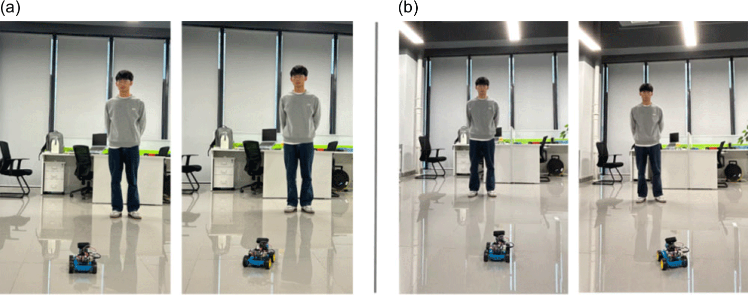
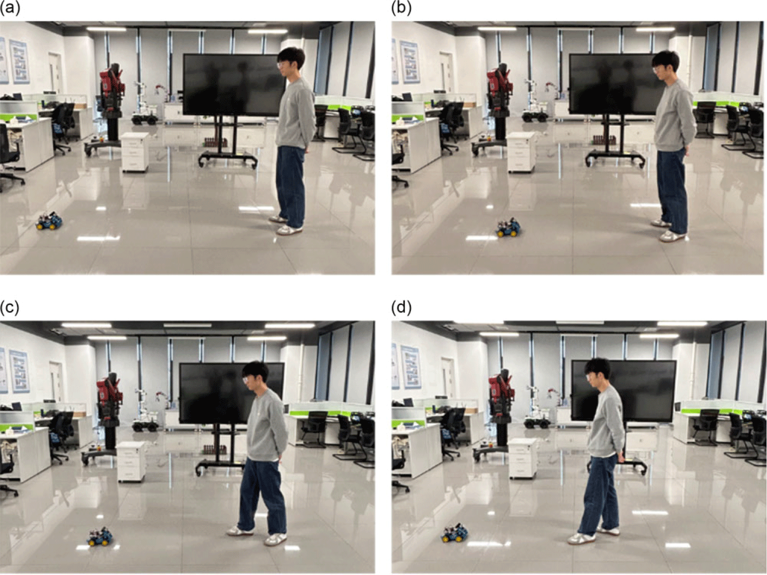
The experimental scenario and process of directional tracking are depicted in Figure 14. In Figure 14(a), the target initially positions at the right front of the robot. Once the robot detects the face and computes the directional deviation, it begins turning right. This continues until the absolute value of the directional deviation is adjusted within the pre-set directional threshold, aligning the robot directly toward the target. This signifies the completion of directional tracking through rightward adjustment.
Direction tracking experiment. (a) Right-turn direction tracking (b) Left-turn direction tracking.

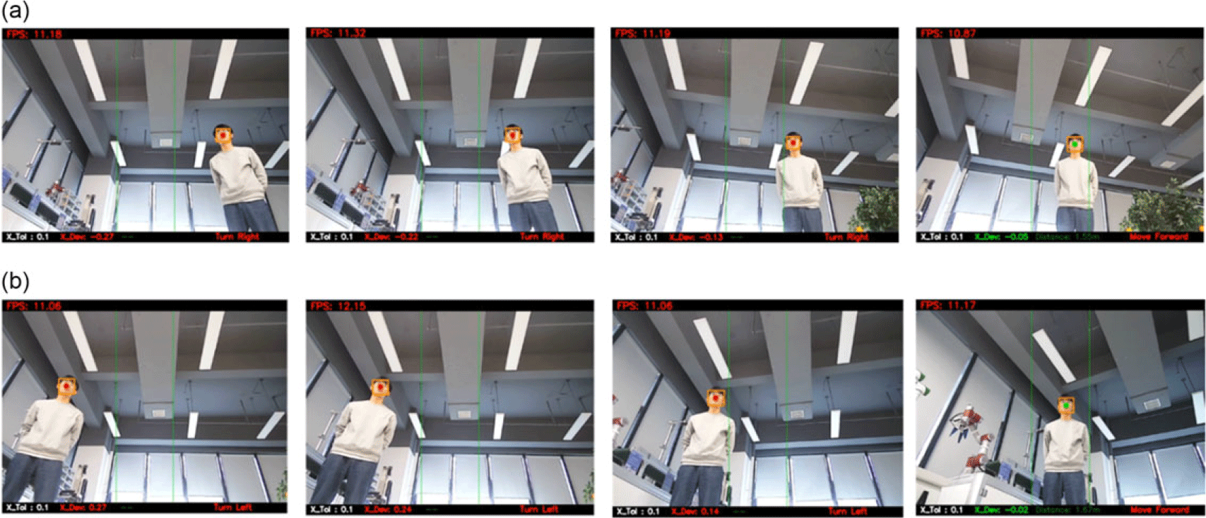
The real-time direction tracking is shown in Figure 15, with a focus on the right-turn direction tracking experiment presented in Figure 15(a). Initially, the tracking target is situated in the robot’s right front, with a directional deviation of
 $X_{Dev}=-0.27$
. This value exceeds the absolute directional threshold, necessitating directional adjustments. As the direction tracking progresses, the directional deviation gradually diminishes, reaching
 $X_{Dev}=-0.05$
, where the absolute value falls below
 $X_{Tol}$
, indicating successful completion of the direction tracking through a right turn. For left-turn direction tracking, refer to the experimental setup and real-time detection shown in Figs. 14(b) and 15(b) respectively. Similarly, the robot detects the face target positioned in front of it on the left, computes the directional deviation, and achieves real-time and effective directional control through left-turn tracking, ensuring precise tracking of the target at all times.
Real-time detection of direction tracking experiment. (a) Right-turn direction tracking (b) Left-turn direction tracking.

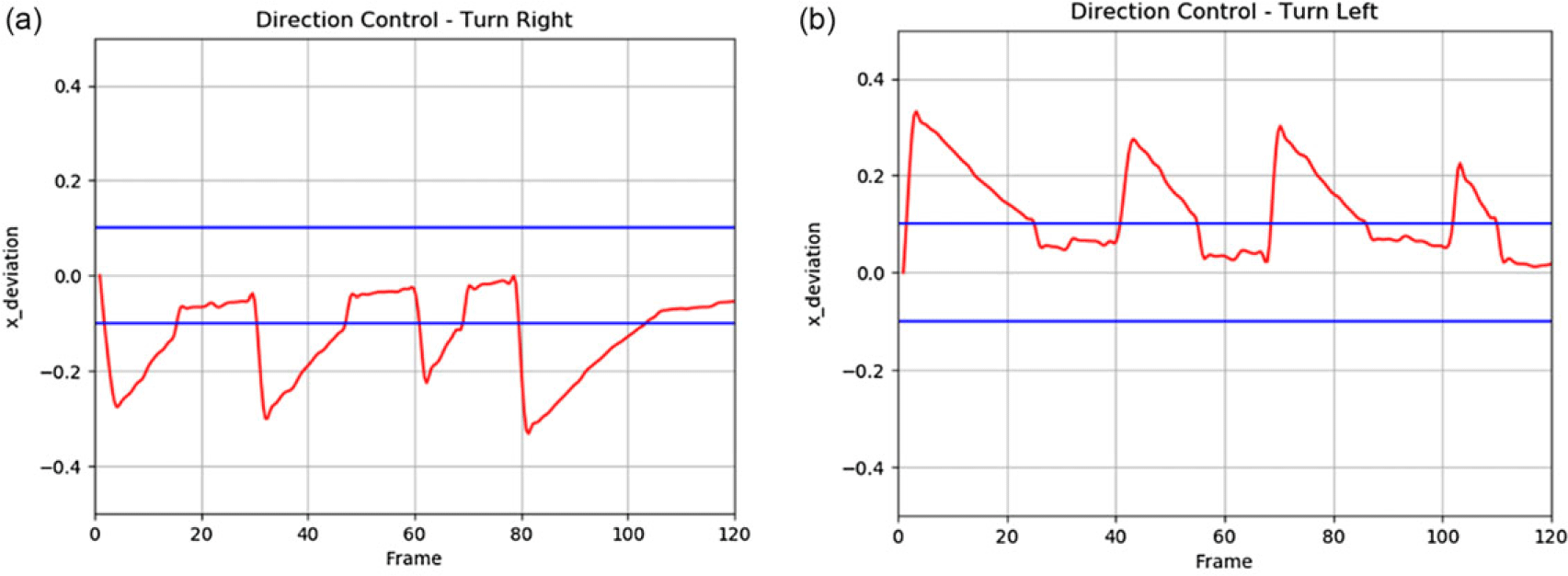
Several experiments were conducted on direction tracking, and real-time deviations were generated by capturing the orientation deviation of the center of the face frame in the X-direction frame by frame during the tracking process. The direction deviations from these experiments are illustrated in Figure 16.
Real-time deviation of direction tracking. (a) Right-turn direction tracking and (b) Left-turn direction tracking.

In the real-time deviation graph, the X-axis represents the number of frames detected and processed, while the Y-axis depicts the real-time deviation of the center of the face frame from the center of the video frame along the X-coordinate. The increment in frames from 0 to 120 illustrates the duration of the face-tracking experiment. Assuming the real-time detection and processing interface operates at approximately 10 frames per second (fps), processing 120 frames corresponds to approximately 12 s. As the number of frames increases, the phase characterized by increasing absolute deviation reflects rapid movement of the target in front of the robot, prompting continuous evaluation of the system’s ability to track the direction of the human face. Conversely, periods where absolute deviation decreases and stabilizes signify the robot’s directional tracking phase, during which directional deviations are adjusted within predefined thresholds. As illustrated in Figure 13, the target continuously adjusts its position in front of the robot, enabling the system to perform real-time face detection, calculate directional deviations, and adjust robot steering accordingly. This ensures precise tracking of the target throughout. Directional tracking experiments confirm the system’s capability to achieve real-time and effective directional tracking based on the strategies outlined in this paper, contingent upon successful face detection by the robot.
3.3.3. Distance tracking experiment
The experimental setup and process of distance tracking are depicted in Figure 17. In Figure 17(a), the face target initially positions directly in front of the robot, and the distance to the robot exceeds
 $D_{\max }=1.5\,{\rm m}$
. Upon detecting this, the robot initiates forward movement to track the target until it reaches a safe distance, then stabilizes its position. Figure 17(b) illustrates a scenario where the target is approaching the robot, and the robot detects that the distance to the target is less than
 $D_{\min }=1.3\,{\rm m}$
. In response, the robot moves backward to avoid collision, ensuring it maintains a safe distance within the range of (1.3 m, 1.5 m).
Forward and backward distance tracking experiment.

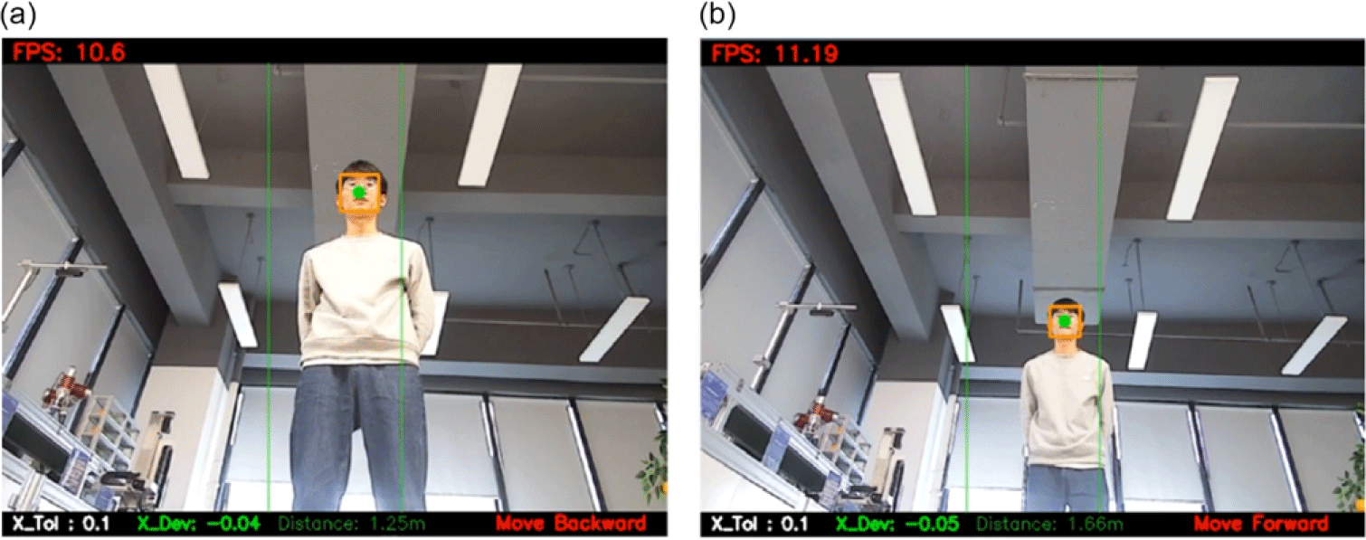
Figure 18 depicts real-time detection of forward-backward distance tracking. In Figure 18(a), the robot measures the distance to the face target as 1.66 m, which exceeds
 $D_{\max }=1.5\,{\rm m}$
, prompting it to move forward to track the target. Figure 18(b) shows the distance measured as 1.25 m, which falls below
 $D_{\min }=1.3\,{\rm m}$
, indicating the robot moves backward to maintain a distance within (1.3 m, 1.5 m) from the target.
Real-time detection of distance tracking.

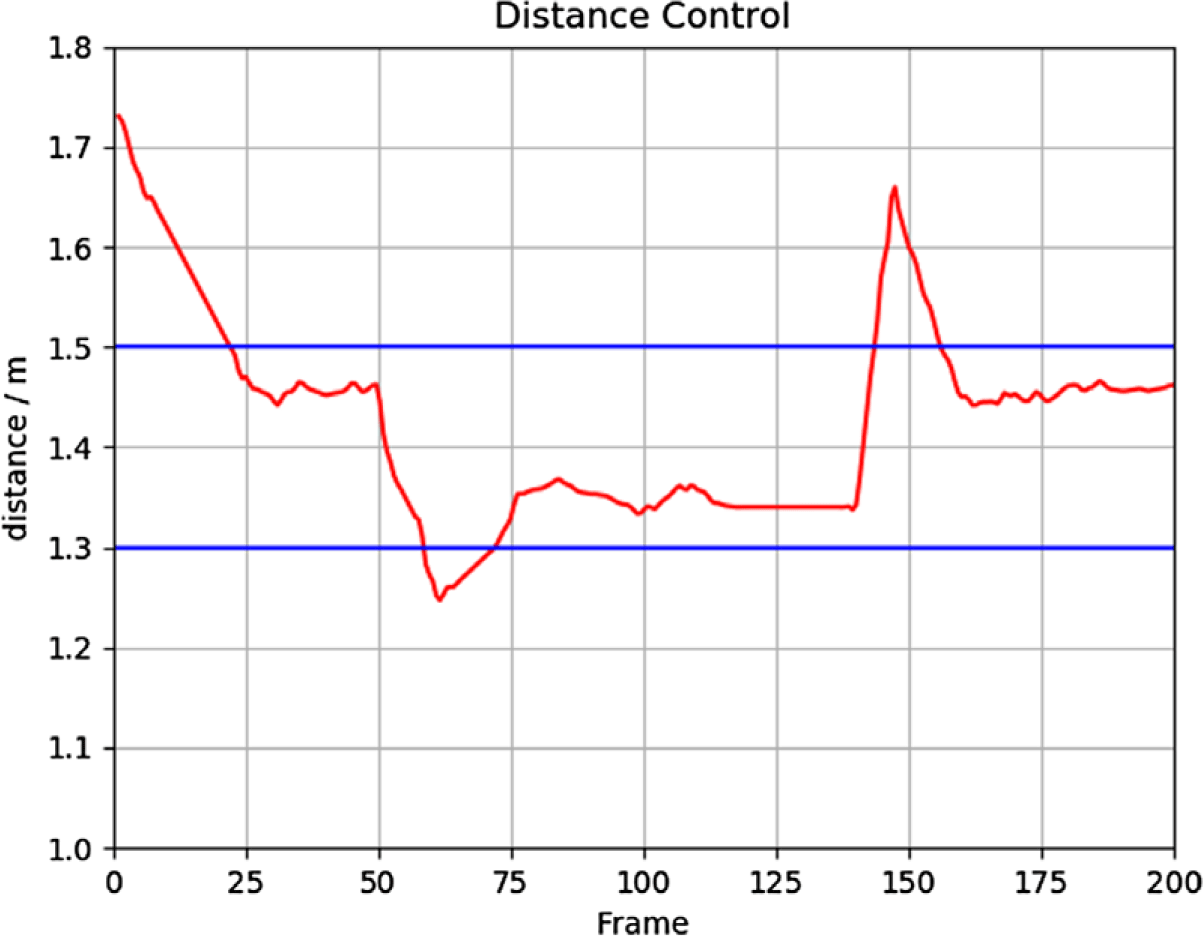
After conducting multiple experiments, the real-time distance between the robot and the target was measured frame by frame during distance tracking. A graphical representation of this real-time distance recording is depicted in Figure 19.
In Figure 19, the X-axis denotes the number of frames detected and processed, with increasing numbers representing the passage of time. Assuming a processing fps of around 10, this corresponds to approximately 20 s for 200 frames. The Y-axis shows the distance between the robot and the tracked target, measured in meters by the ultrasonic sensor. Two blue lines represent the predefined safety distances,
 $D_{\min }$
and
 $D_{\max }$
respectively. As depicted in Figure 17, regardless of whether the tracked target approaches or moves away from the robot, ensuring the distance between them does not fall within the range
 $(D_{\min },D_{\max })$
, the system described in this paper can effectively control the robot. This control is achieved by adjusting its forward and backward movements to maintain a safe distance from the target, thereby achieving effective distance tracking.
The distance tracking experiment demonstrates that accurate measurement of the distance to the following target can be achieved using an ultrasonic sensor. The tracking strategy proposed in this paper enables effective distance tracking, allowing the robot to maintain a safe distance from the target and ensuring precise distance tracking control.
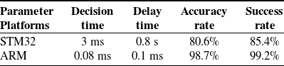
Algorithm performance on different hardware platforms.

Real-time distance recording for distance tracking.

Based on the experiments and data analysis above, it is evident that the multi-sensor combination-based face-tracking strategy proposed in this paper successfully generates precise and effective tracking commands. This capability enables the mobile robot to perform real-time and effective motion tracking of detected face targets. The experimental results validate that the face detection and tracking control system proposed in this study achieves offline real-time, high-precision face detection and efficiently tracks detected face targets with accuracy.
To verify the versatility and superiority of the proposed algorithm, tests were conducted on different hardware platforms. The algorithm was loaded onto the STM32 and ARM, and the performance test results are shown in Table IV. According to the test results, due to the smaller memory and weaker task processing capability of the STM32, it was unable to complete the tasks effectively. In contrast, the ARM performed better than the Raspberry Pi, enabling it to complete the tasks more efficiently. The experimental results demonstrate that the proposed algorithm has a certain degree of versatility.
4. Conclusion
This paper focuses on two technologies in mobile robot target tracking control, namely target recognition and tracking control. It mainly studies target detection algorithms based on deep learning and MPC tracking control algorithms and considers the limited computational performance of mobile robots by optimizing and improving the algorithms. A four-wheeled differential drive mobile robot based on Raspberry Pi 4B was built as an experimental platform to validate the mentioned algorithms. The main contributions of this paper are:
(1) This paper proposes an efficient lightweight method for target recognition based on an enhanced version of RetinaFace. The approach employs a backbone network utilizing depthwise separable convolutions for feature extraction and incorporates an ECAM. This module reduces the impact of redundant features while emphasizing crucial channels, thereby decreasing model complexity and enhancing network efficiency.
(2) To address the issue of a single visual sensor being unable to accurately measure distance in servo tracking tasks, this paper proposes a simple and effective tracking method that integrates both vision and ultrasonic sensors. This approach effectively leverages the strengths of both sensors: the visual sensor’s directional sensing capability and the ultrasonic sensor’s accurate distance measurement.
Experimental results demonstrate that the proposed method outperforms RetinaFace average precision by 1.2%, 1.4%, and 1.1%, respectively. Also, the model size is only 1.71 MB, which can realize high-precision and fast face detection in Raspberry Pi 4B. Furthermore, it effectively tracks detected targets during motion with stability and reliability.
Although the proposed algorithm achieves lightweight implementation and improves target recognition accuracy, it has only been tested in simple scenarios and does not address complex situations involving obstacles, occlusions, or other challenging environments. Future research will incorporate factors such as obstacle avoidance into the tracking control, aiming to enhance the adaptability and safety of mobile robots in complex environments.
Author contributions
Yiming Hua and Xiang Cao conceived and designed the study. Haoxiang Li conducted data gathering. Xueyou Huang performed statistical analyses. Yiming Hua, Xueyou Huang, Haoxiang Li, and Xiang Cao wrote the article.
Financial support
This work was supported in part by the National Natural Science Foundation of China under Grant 62473002, 61773177, 61921004, 62303009, the Natural Science Foundation of Anhui Province under Grant 2308085MF204, the University Industry-university Research Innovation Fund of China under Grant 2021ZYA11013, and the Open Research Project of the Anhui Provincial Key Laboratory of Security Artificial Intelligence under Grant SAI202401.
Competing interests
The authors declare that they have no known competing financial interests or personal relationships that could have appeared to influence the work reported in this paper.
Ethical approval
Not applicable.