


In politics, personal identity matters. A lot. Would the United Kingdom have had a season of privatization without the leading role of Margaret Thatcher, or the United States a New Deal without Franklin Delano Roosevelt? And what would have happened to the United States had Robert Kennedy become its 37th president? A recent literature has recognized the crucial relevance of the identity of leading politicians in taking policy decisions and ultimately in shaping the development of their party or the entire nation (e.g., see Jones and Olken Reference Jones and Olken2005; Dewan and Myatt Reference Dewan and Myatt2007; Reference Dewan and Myatt2008). Similar considerations on the crucial role played by leading persons (that is, CEOs) apply also to the business sector (e.g., see Bertrand and Schoar Reference Bertrand and Schoar2003).
If identity matters, selecting good politicians becomes ever more crucial. But how to achieve an efficient process of political recruitment? Does electoral competition improve political outcomes (see Stigler Reference Stigler1972; Wittman Reference Wittman1989) by leading to the selection of better politicians?
To address these questions, we introduce a model of political selection in a majoritarian system, characterized by plurality rule in single-member districts. Rather than analyzing the self-selection of political candidates, we concentrate on the selection of politicians by parties (leaders). Potential candidates differ in their valence (or quality), which is perfectly observable and is valued by all voters (see Stokes Reference Stokes1963; Reference Stokes and Kavanagh1992; Enelow and Hinich Reference Enelow and Hinich1982; Groseclose Reference Groseclose2001), but is costly for the parties. An original feature of our model is allowing the parties to target specific districts—which differ in their contestability or marginality—by allocating candidates of a particular valence. Thus, in contrast to many existing contributions in the literature, we focus on the effect of political competition on the primal party decision, that is, the selection and allocation of politicians, rather than on the policy choice. Our theoretical model predicts that electoral competition has beneficial effects, because parties choose more high-valence politicians and send them to the most contestable districts.
To test this prediction, we use a recent dataset on all Italian members of parliament elected in majoritarian (single-member) districts from 1994 to 2006. In that period, Italy represented the perfect testing ground for our theoretical model for several reasons. First, parties (leaders) played a crucial role in the recruitment of political candidates. Second, a majoritarian system was used to elect one of the largest assemblies in the world. Third, for historical reasons, there was large geographic variation in the ideological strongholds of the two major political coalitions (center-right versus center-left). All of these features provide a considerable amount of within-country variation in the degree of political contestability. We use this variation as the treatment of interest and evaluate its effect on political selection.
In particular, to measure the degree of political contestability of a single electoral district, we construct two different indicators: (i) the margin of victory in the previous political election and (ii) the district-specific ratio of the number of swing voters to the difference between the ideological voters of the two main coalitions. The latter indicator is estimated using electoral data from the previous European elections, which take place under a proportional system and are largely believed to capture ideological voting.
Valence is captured by multiple measures: years of schooling, previous market income, and past experience in local governments. The rationale for each measure is simple. Years of schooling capture the acquisition of formal human capital and skills. Preelection income, controlling for the occupational type, is a measure of market success and ability. The use of administrative experience is linked to the idea that lower-level elections can be used by high-quality politicians to build reputation and by voters to screen better candidates.Footnote 1
Consistent with our theoretical framework, we find evidence of an ex ante selection effect of political competition: politicians with more years of schooling, higher preelection income, and more local experience tend to be allocated to contestable (nonsafe) districts. Indeed, the two main political coalitions show on average very different patters of political selection: the center-right coalition tends to recruit politicians with higher education, and the center-left to select more women and more politicians with previous administrative experience. However, evidence from a regression discontinuity design shows that both parties converge to the same high-valence type in close electoral races. In other words, when the going gets tough, the tough candidates get the job from their parties.
To capture ex post quality of the elected officials, we consider the absenteeism rate in electronic parliament votes, which we consider a proxy for shirking or rent-seeking.Footnote 2 Our empirical evidence shows that politicians elected in contestable districts display a lower absenteeism rate. This is consistent with the selection of better politicians in those districts, but may also be driven by reelection incentives. To disentangle the two channels, we exploit some (exogenous) changes in political alliances forced by national leaders, which had the effect of altering the degree of contestability of some local districts from one election to the next.Footnote 3 Interestingly, we find that the effect of political selection strongly dominates, because the ex ante contestability of the district has a sizable impact on performance even when we control for the change in reelection incentives. An incentive effect does exist, however, particularly for low-valence politicians, as we find that, when a safe district turns contestable, low-valence incumbent politicians tend to exert more effort.
Our results hence point to the existence of a positive effect of political competition on the selection of politicians in a country—Italy—characterized by a majoritarian electoral rule and by strong parties featuring fairly centralized recruitment of candidates for parliament. However, a positive association between the ex ante quality of politicians and political competition can be expected to hold also in majoritarian environments with strong parties but local recruitment patterns, such as the United Kingdom, or even with a weak party structure, such as the United States. The last case may occur if voters at primary elections select their party's candidates by trading off ideological loyalty for better skills, in order to attract independent voters at the general election. More generally, whenever the electoral race is tight and unaligned voters care about the personal attributes of candidates, we expect to observe competition on good politicians. From a normative perspective, our findings thus call for institutions and policies able to (i) increase voters' information and awareness about the valence of political candidates and (ii) enhance the degree of contestability of electoral races.
RELATED LITERATURE
Our paper is related to several strands of the literature. The theoretical framework shares some features with the models in Groseclose (Reference Groseclose2001) and Besley and Preston (Reference Besley and Preston2007). Two ideological parties compete for the votes of ideological and of swing voters. The degree of political competition depends on the distribution of these voters across electoral districts. In contrast to Besley and Preston (Reference Besley and Preston2007), where parties choose an economywide policy and are unable to target specific districts, our novelty is to assign to the parties the primal role of selecting candidates and of allocating them to electoral districts. This allocation decision is crucial, because it allows the parties to target specific districts. And, in our setting, when it comes to elections “all politics is local” (Jacobson Reference Jacobson1989).
In our model, candidates differ in their valence (see Groseclose Reference Groseclose2001; Besley Reference Besley2005), such as their ability or expertise in problem solving.Footnote 4 On valence (or competence), all voters share identical views, as they all prefer more to less (see Stokes Reference Stokes1963; Reference Stokes and Kavanagh1992). However, because parties have different (exogenous) ideological positions, valence becomes crucial in determining the choice of the nonideological voters. In our framework, ideological parties thus choose valence in order to win the election. Our model borrows from recent literature that has examined the relation between party ideology and candidate valence. Groseclose (Reference Groseclose2001) shows that the party with the candidate enjoying an exogenous valence advantage will choose to be more moderate, because this advantage becomes more relevant for lower ideological differences (see also Ansolabehere and Snyder Reference Ansolabehere and Snyder2000; Aragones and Palfrey Reference Aragones and Palfrey2002). In our model, valence is more relevant for nonideological voters. Building on this intuition, Ashworth and Bueno de Mesquita (Reference Ashworth and Bueno de Mesquita2007) endogenize both valence and ideology to show that in equilibrium, parties choose to diverge in policy in order not to compete on (costly) valence. Other models of joint determination of valence and ideology include Schofield (Reference Schofield2003) and Dickson and Scheve (Reference Dickson and Scheve2006).
Our model concentrates on the choice of political candidates by the party. This demand for politicians has largely been neglected in the theoretical literature, despite the predominant role played by (strong) political parties in most contemporaneous democracies. Among the few contributions, Carrillo and Mariotti (Reference Carrillo and Mariotti2001) analyze the party decision between an experienced, and thus known, incumbent and a new candidate of uncertain quality in an asymmetric information setting, to show that parties may have an incentive to confirm mediocre incumbents. Mattozzi and Merlo (Reference Mattozzi and Merlo2010) focus on the recruitment of political candidates by two parties competing in an election. In their framework, parties may find it optimal to attract low-quality politicians, in order to keep the overall level of party service sufficiently high.Footnote 5
A recent literature examines the effect of political competition on policy outcomes. Besley, Persson, and Sturm (n.d.) use different measures of the degree of political competition in U.S. local elections, and find evidence of a positive effect of competition on growth-enhancing policies and, ultimately, on economic growth. Stromberg (Reference Stromberg2008) analyzes how U.S. presidential candidates allocate resources across states to maximize their probability of winning the election, and shows that this allocation is affected by the number of electoral votes and forecast uncertainty. Dal Bo, Dal Bo, and Snyder (Reference Dal Bo, Dal Bo and Snyder2009) show that political dynasties (that is, intergenerational transmission of political power and elected offices) are less likely to emerge in competitive environments.
Few empirical studies have studied the importance of candidates' valence for electoral competition. Shugart, Valdini, and Suominen (Reference Shugart, Valdini and Suominen2005) study personal vote-earning attributes under proportional representation. The quality of candidates—measured as local birthplace and lower-level electoral experience—is shown to decline with district magnitude when lists are closed, because quality becomes less useful to parties. In contrast, quality increases with district magnitude when lists are open, because competition gets tighter. Jacobson (Reference Jacobson1989) also measures candidates' valence as previous experience in any elective public office. He shows that high-quality candidates in the United States decide to run for office only when national conditions favor their party, and that they are able to win more votes for their party, even controlling for the initial favorable conditions that motivated their self-selection decision. Analogously, a recent paper by Atkinson, Enos, and Hill (Reference Atkinson, Enos and Hill2009) shows that challengers with higher (perceived) facial competence are more likely to run in more competitive districts. Moreover, their higher facial competence positively affects the vote choice of the unattached voters. Stone, Maisel, and Maestas (Reference Stone, Maisel and Maestas2004) investigate the impact of incumbent's valence on political competition. They extend the logic of Black's (Reference Black1972) “strategic politicians” thesis and use survey data on potential candidates in the United States, to show that a high (perceived) valence of the incumbent deters the entrance of strong challengers. Finally, Green (Reference Green2007) presents aggregate trends to suggest that British political competition has become more competence-based, because the major parties (as well as the electorate) have converged on the ideological (left–right) dimension.
THE MODEL
Our model describes the selection and allocation of political candidates into electoral districts by two parties that compete in a majoritarian election. The two parties, D and R, are ideological, and have different bliss points over a national policy, respectively Ŷ D < Ŷ R. The role of the party (leaders) before the election is to select and allocate candidates into the electoral districts. After the election, the winning party i sets its most preferred national policy, Ŷ i; and each winning candidate provides constituency service for his/her district.
Candidates differ in their valence, which can be high or low. Voters prefer high to low valence. High-valence candidates are called “experts” to convey the idea that they are better equipped at problem solving; this expertise is valued by all voters. Low-valence politicians are called loyalists (to a party) to suggest that their ability is in providing party services; hence it is valued by the party, but not by the voters. Each party i selects a share μi of experts (and residually 1−μi loyalists) to allocate to the different districts. Because parties are ideological and care about the national policy, they will use their selection and allocation decisions to try to win the election. Recruiting experts is costly for the parties (see below for a more detailed discussion of this point).
Voters care about the national policy and the valence of the candidates in their district. They can be of three types: ideological supporters of either party's national policy (D and R), or centrist (C), that is, not aligned to any party. Voters in groups D and R are core supporters, and always vote respectively for parties D and R, regardless of the valence of the two parties' local candidates. We embed the voting decision of the centrist (group-C) voters in a standard probabilistic voting model (see Lindbeck and Weibull Reference Lindbeck and Weibull1987). Being unaligned, centrist voters strongly care about the valence of the candidates in their districts. Hence, the decision of where to allocate the experts carries important implications for winning the election. The utility that group-C voters living in district k derive from the policy selected by party i and from candidate-i valence is summarized by the expression

where v C(Y i) is the utility deriving from party-i national policy (or ideology), V C(y ik) with y ik ∈ {E i, L i} is the utility from the valence of party-i candidate in district k, depending respectively on whether he/she is an expert (E i) or a loyalist (L i); and ρ measures the relative importance to the voters of the local candidate valence versus the national policy. We assume symmetry in the two parties' bliss point and in the centrist voters' preferences, so that v C(Ŷ D) = v C(Ŷ R). Furthermore, centrist voters prefer to have expert candidates in their districts: V C(E i) > V C(L i).
Following the probabilistic voting approach, we assume that each of these centrist voters may feel ideologically closer to one party or another. The ideological characteristic of each centrist voter is indexed by s, with s > 0 if the voter is closer to party R, and vice versa. The distribution of ideology among centrist voters is assumed to be uniform. In particular, to simplify the notation, we consider s ~ U[-1/2,1/2]. The centrist voters' decision is also affected by a common popularity shock to the parties, which occurs before the election and may modify the perception, δ, that all centrist voters have of the image of the two parties. In particular, if δ > 0, party R gains popularity from this preelectoral popularity shock and vice versa for δ < 0. To simplify the algebra, we assume that δ is uniformly distributed, so that δ ~ U[−1/2ψ, 1/2ψ] with ψ > 0.Footnote 6
To summarize, a centrist voter will support party D if the utility obtained from the party-D national policy and from party-D candidate in the district is larger than the sum of the ideological idiosyncratic component, s, of the common shock, δ, and of the utility obtained from party R. That is, a centrist in district k prefers D if U kC(Y D, y Dk) − U kC(Y R, y kR) − s − δ > 0.
Voters and Districts
The distribution of the three groups of voters in the electoral districts determines the districts where the electoral race is tight, and those where instead one of the two parties has a substantial advantage. Call λjk the share of type-j voters in district k with j ∈ {D, C, R}. We assume that the share of type-C voters is constant across districts, that is, λCk = λC∀k.
It is convenient to define our measure of ex ante contestability of every district k as

When parties D and R have an equal share of aligned voters in the district—and hence there is maximum electoral contestability—this index is equal to zero; whereas higher (positive) and lower (negative) values indicate less contestability. Moreover, it is easy to see that party D always wins in those districts with λk < −1/2, in which group-D voters represent a majority of the electorate; whereas party R always prevails in districts with λk > 1/2. Hence, only districts with intermediate values of λk ∈ [−1/2, 1/2] are contestable. To characterize the distribution of voters type across districts, we consider a continuum of districts, characterized by a degree of contestability, λk, that is uniformly distributed around λk = 0, with a support λk ∈ [−(1− λC)/2λC, (1−λC)/2λC].Footnote 7 We refer to the cumulative distribution as G(λk).
We are now in the position to assess the probability that a party—e.g., party D—wins a contestable district k. Call  the ideology of the swing voter, that is, of the centrist voter who is indifferent between party D or R. Hence, = U kC(Y D, y kD) − U kC(Y R, y kR) − δ, and all centrist voters with ideology s < will support party D. To win district k, the sum of type-D voters (λkD) and of the votes that party D obtains from the centrist voters has to exceed 50%. It is easy to see that this occurs for > λk. Thus, the probability of party D winning district k—call it ΠDk—can be expressed as a function of the popularity shock, δ, and of the district characteristic, λk:

where d k can be interpreted as a measure of the ex post contestability of district k; that is, after that the parties' national policy and allocation of candidates are known to the voters. Because the popularity shock is uniformly distributed with density ψ, we can rewrite equation (3) as ΠkD = 1/2+ψd k. If the two parties converge to the same allocation of candidates, because the national policies provide the same utility to the centrist voters, then d k=−λk. However, parties can use the allocation of candidates to modify d k, and thus their chance of winning district k.
Selection and Allocation of Candidates
To understand the selection and allocation of candidates into districts, it is convenient to summarize the timing of events. Before the election, parties take selection and allocation decisions in two stages. First, they select their shares of expert and loyal candidates, respectively μi and 1 − μi. Second, they choose how to allocate them into the different electoral districts. At each stage, the two parties may take their decisions independently and simultaneously; they know the distribution of the popularity shock taking place before the election, but not its realization. After the popularity shock has occurred, centrist voters decide whom to support between the two candidates running in their district. After the election, the winning party sets its most preferred national policy, and the winning candidate delivers constituency service according to his/her valence.
Because parties are ideological and have preferences over the national policy, they have an incentive to win the election in order to be able to set their most preferred policy. To do this, they use their selection and allocation decisions. Experts increase the probability of winning districts, and hence the election, but have a recruitment cost. Parties will hence compete by selecting and allocating experts to the crucial districts, in order to maximize their expected utility. For party D, the expected utility is

where ΠD, party D probability of winning the election, depends on the selection and allocation of candidates, v D(Y i) is the utility deriving from party-i national policy, and C(μD) represents the cost associated with having a share μD of experts in the party list. In particular, we assume a linear cost function, C(μ) = γμ, where γ can be interpreted as the extra wage to be paid to an expert candidate, relative to a loyalist. This additional wage may arise because of experts having better outside options in the labor market (see also Mattozzi and Merlo Reference Mattozzi and Merlo2008). Alternatively, C(μ) can be interpreted as the foregone rents for the party associated with having more experts and hence fewer loyalists, who would have provided more party services, and thus higher rents for the party. The expected utility of party R, u R, is defined analogously.
To analyze the parties' decisions on the selection and allocation of candidates, it is convenient to work backward. First, we consider a fixed number of experts in the party list, and examine their allocation into the different districts. Second, once the allocation of experts is determined, we characterize the share of experts in the party list that maximizes the expected utility at equation (4). Notice that at each stage the two parties take their decisions simultaneously and independently.
Allocation of Candidates
Consider a fixed share of experts for parties D and R, respectively μD and μR, to be allocated. The difference in utility provided to the centrist voters in district k by the two parties can be written as

As experts are more valuable than loyalists to centrist voters, allocating an expert to a district k, where the other party sent a loyalist, amounts to increasing the centrist voters' utility by a positive wedge, W = ρ[V C(E) − V C(L)]. More centrist voters in that district will then favor the party that allocated the expert. Hence, parties compete on good politicians (experts) to increase their probability of winning a contestable district.
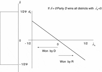
To understand the logic behind this simultaneous allocation game, suppose that only loyal candidates have been sent to districts, and are thus perfectly matched; that is, every party-D loyalist faces a party-R loyalist. This implies that V C(y kD) − V C(y kR) = V C(L) − V C(L) = 0. By equation (3), party D thus wins a district k if the shock is δ < d k = − λk. Moreover, given the distribution of districts (λk), party D wins the election—that is, it obtains more than 50% of the districts—if the shock is strictly in its favor: δ < d 0 = 0. In this case, party D wins all the districts with λk < 0, as shown in Figure 1; whereas it ties the election for δ = d 0 =0.
Allocation Game, Distribution of Districts, and Common Popularity Shock

Thus, the marginal districts to win are in a small interval around λk = 0 (henceforth, district zero, i.e., λ0). It is convenient to represent a small district interval around λ0 as [λϵ, λΞ], with λ0 − λϵ = λΞ − λ0 = ϵ small enough.
Suppose now that party D sends experts to the district interval [λ0, λΞ]. Using again equation (3), it is easy to see that party D is now more likely to win districts [λ0, λΞ]. In fact, party D wins district λ0 even for a less favorable (i.e., larger) realization of the shock, that is, for δ < W. Define the district λw = − W, such that d w = W. Then, if party D allocates an expert to the most contestable district, λ0, where party R has instead sent a loyalist, party D wins this district with the same probability with which it wins district λw < 0 (which is ex ante biased in favor of party D) when both parties send a loyalist. Hence, for δ = d 0 = 0, with experts in the district interval [λ0, λΞ], party D would win the election, rather than just tying it. Analogously, if party R allocates an expert to the most contestable district, λ0, whereas party D sends a loyalist, party R's probability of winning district λ0 will equate the probability of winning district λW = W, such that d W = −W, when both parties allocate a loyalist there.
Districts λw and λW represent important thresholds, for party D and R respectively. To see this, suppose that party R allocates experts everywhere; then party D would minimize its probability of losing the election by sending experts to the districts between λw and λΞ. In this case, party D would win the election if δ ≤ 0, and hence with probability 50%. Moreover, allocating an additional expert to any district would not modify this probability. We call this allocation choice by party D a “defensive” strategy, because party D protects—by sending experts—the contestable districts biased in its favor (those between λw and λ0), and places only few, yet crucial, experts on its opponent's turf (i.e., in the districts between λ0 and λΞ). With an “offensive” strategy, party D would have placed most (or all) of its experts in the contestable districts biased against it (those between λ0 and λW). It is convenient to define the mass of districts included between λw and λ0 as η/2; that is, [G(λ0) −G(λw)] = η/2. Hence, η/2 experts are enough for party D to span the districts between λw and λ0, and thus to have a defensive strategy. The same logic applies to party R, with the threshold district being λW, and [G(λW) − G(λ0)] = η/2. Notice that the mass of crucial districts between λw and λW is equal to η =[2λC/(1−λC)]W. The share of experts needed to cover all the crucial districts thus depends positively on the proportion of centrist voters (λC), on the relative importance that they give to the local policy (ρ), and on the value that they attribute to having an expert in their district, V C(E) − V C(L).
The next proposition describes the allocation strategy chosen by the two parties (a formal version of Proposition 1 with a detailed description of the allocation of experts into districts is provided in the Appendix).
Proposition 1. If both parties have enough experts, μi > η/2, i = D, R, they both play a “defensive” strategy, which consists of placing experts in their own contestable districts and around the most contestable one; if only one party has enough experts, it will adopt an “offensive” strategy, by placing its experts in the other party's contestable districts and around the most contestable one, whereas the opponent party will match the experts around the most contestable one.
When neither party has enough experts, μi < η/2, i = D, R, and their shares of experts are comparable in size, they both play an “offensive” strategy, by allocating experts in the other party's contestable districts; whereas when neither party has enough experts but one party largely dominates in the share of experts, the dominant party will use an “offensive” strategy, and the weak party will try to match the experts in its own contestable districts.
The above proposition suggests that, with enough experts, both parties can defend their districts and ensure a 50% probability of winning the election; however, they cannot improve upon that. When this defensive strategy is instead unavailable to one of the parties, the strong party will have an incentive to attack the districts biased in favor of the weak party by sending experts; and the weak party will try to match these experts in an attempt to minimize the probability of losing the election. When neither party has enough experts to defend its competitive districts, they will both have an incentive to attack the other party's districts by sending their experts there. If, however, one party has an advantage in share of experts (despite not having enough of them), it will use the offensive strategy to raise its probability of winning above 50%, whereas the weak party will try to match its experts in its own districts to minimize the probability of losing the election.
Selection of Candidates
Once we know how candidates are allocated across districts, we can turn our attention to the selection of the relative shares of experts and loyalists. The objective of party D (leaders) is to maximize expected utility at equation (4), and analogously for party R. The selection of experts may increase the probability of winning the election, but at a cost, because experts have to be rewarded with an extra wage, γ.
It is useful to define the difference in utility for party D when the national policy is set by this party (ŶD) or by the opponent (ŶR) as Δv D = v D(ŶD) −v D(ŶR). Analogously for party R, we have Δv R = v R(ŶR) −v R(ŶD). Due to symmetry, we have Δv R = Δv D = Δv. The next proposition describes the equilibrium selection and allocation strategy by the two parties, for a sufficiently low cost of acquiring an expert.
Proposition 1. For γ < [(1−λC)/λC]ψΔv, the equilibrium share of experts chosen by both parties is μD = μR = η/2+ϵ. The corresponding allocation of experts is [λw, λXi] for party D, and [λϵ, λW] for party R. Hence, experts are always elected in the most competitive districts [λϵ, λXi]. Both parties win the election with equal probability, ΠD = ΠR = 1/2.
To see the intuition for the result, suppose that party R has selected only a few experts, μR < η/2. If the cost of the experts, γ, is sufficiently low, party D will have an incentive to choose a larger share of experts in order to push its probability of winning the election above 50%, and therefore to increase its expected utility. For a sufficiently low γ, party D will find it convenient to increase its probability of winning the election by having μD = η/2+ϵ experts. And so will party R. When a party has selected (and properly allocated) η/2 + ϵ experts, the opposing party cannot increase its probability of winning the election above 50%, and any additional expert above the share of η/2 + ϵ would thus represent a pure cost bringing no additional benefit. This allocation implies that both parties send experts to the most competitive districts; as a result, in the interval [λϵ, λΞ], only experts are elected.
The equilibrium share of experts thus largely depends on the competitiveness of the political system. In particular, as stated in the next proposition, a majoritarian electoral system with a larger number of competitive districts is associated with a larger share of experts selected (and allocated) by the competing parties.
Proposition 3. An increase in the share of centrist voters (λC) increases the equilibrium share of experts chosen by both parties, μD = μR = η/2 + ϵ, as long as the following condition holds: γ < [(1−λC)/λC]ψΔv.
The intuition behind this proposition is straightforward. An increase in the share of centrist voters (λC) increases the share of contestable districts, η, and therefore also the share of experts needed in equilibrium to cover these districts. However, an increase in λC reduces the impact that adding few more experts has on the probability of winning the elections. To the extent that the cost of the experts is sufficiently low, despite this reduction, the marginal benefit of adding experts still overweights its cost, and parties will choose to span all η/2 + ϵ crucial districts, and will thus increase their equilibrium share of experts.
ITALIAN INSTITUTIONS AND POLITICS FROM 1994 TO 2006
In order to test the main empirical implication of our theoretical model, we use data about the members of the Italian parliament (House of Representatives and Senate) from 1994 to 2006, which refer to legislative terms XII (1994–96), XIII (1996–2001), and XIV (2001–06). During this period, Italy experienced a mixed electoral system (75% majoritarian and 25% proportional). In the majoritarian tier, members of parliament were elected in single-member districts with plurality voting. In the proportional tier, they were selected from closed party lists at the regional level (House) or from the best losers in the majoritarian districts (Senate).
The switch in 1994 from an open-list proportional system to a mixed-member rule was accompanied by major political changes, including the breakdown of the existing party system that followed judicial scandals for corruption charges involving the leaderships of all government parties.Footnote 8 As a result, the 1994 elections featured new parties competing under the mixed electoral system. A right-wing coalition led by Silvio Berlusconi, which included his party, Forza Italia, together with Lega Nord, Alleanza Nazionale, and Centro Cristiano Democratico, won the general election with 42.8% of the votes, and 57% of the seats in the House. A year later, a political crisis in the center-right coalition, initiated by Lega Nord (the separatist movement founded and led by Umberto Bossi), brought down the first Berlusconi government, and led to a one-year-long “technical” government by Lamberto Dini (a former minister in the Berlusconi government). In 1996, Lega Nord ran alone in the general election, securing 10% of votes at the national level, a remarkable result for a party with a strong regional base. The elections, however, were won by the center-left coalition Ulivo (Olive Tree), led by Romano Prodi. Like the first center-right alliance, Ulivo resembled more an electoral cartel plagued by internal competition, rather than a government coalition (see Di Virgilio, Reference Di Virgilio1998). In 1998, the leftist Rifondazione Comunista, which was part of the center-left electoral coalition, but had not joined the cabinet, caused the fall of the Prodi government. The center-left coalition managed to survive for the rest of the term by forming three other cabinets, but—without Rifondazione Comunista—lost the next general election in 2001. It was again the turn of Silvio Berlusconi and his center-right coalition (this time including Lega Nord) to rule the country until 2006, which is the end of our sample period.Footnote 9
The introduction of a mixed electoral system did not reduce the dominance of party organizations in Italian politics, as they maintained a firm grip over the recruitment of political candidates in both the majoritarian and proportional tiers. In contrast to other political systems characterized by single-member districts, Italy displayed a centralized process of candidates' selection, where party leaders exercised direct control over nominations, rather than leaving discretion to local party branches. In fact, very few representatives were rooted in a particular constituency (see Di Virgilio Reference Di Virgilio1998; Ferrara Reference Ferrara2004b). The selection and allocation game described in our model thus provides a close representation of this political recruitment process. Furthermore, Italy represents the ideal testing ground for the main prediction of our model, because of other peculiar features of the institutional and political framework, namely: (i) the 75% majoritarian electoral system in place from 1994 to 2006 was fairly isolated and not contaminated by the 25% proportional tier (see Ferrara Reference Ferrara2004a); (ii) Italy has one of the largest legislative assemblies in the world (945 members of parliament against, for instance, 535 in the United States or 575 in France); (iii) there exists a large geographic variation in the ideological strongholds of the center-right and center-left coalitions. These features provide a considerable amount of within-country variation in the degree of political contestability of electoral districts, which allows us to evaluate the impact of political competition on political selection as predicted by Proposition 2 in our model.
DATA SOURCES AND VARIABLES
We use data on all Italian members of parliament (House and Senate) elected in single-member districts in the general elections of 1994, 1996, and 2001. In each district, one representative was elected by simple plurality according to a pure first-past-the-post election. The original sources used to collect the data include the Annals of the Italian Parliament (La Navicella) for demographic information, as well as professional and political experience; the Archive of Tax Returns of the members of the Italian Parliament (Servizio Prerogative e Immunità) for income information; and the Italian Parliament Press Office (Ufficio Stampa) for data on individual attendance at voting sessions.Footnote 10
The dataset contains detailed information on the following political and demographic characteristics: self-declared demographics (age, gender, place of birth, place of residence, level of education, field of education, previous job, and marital status); political experience (this includes being a member of the executive committee of a party at the local, regional, or national level; past and current appointments as minister or state secretary; past appointments at the local government level, such as municipality, province, or region; past appointments in parliament); current appointments in the government or in parliament (whether or not a politician is in a second committee, and whether or not he/she is president or vice president of the parliament or of a single committee); political party affiliation; district of election; and coalition type (i.e., majority versus opposition coalition). The dataset also contains yearly total income information, as reported in individual tax returns, as well as information on absences in floor voting sessions, not attended without any legitimate reason.
Measuring Political Competition
We decided to restrict our analysis to politicians elected in majoritarian districts, because for them we can measure the degree of political contestability, that is, the expected electoral gap between the two major political coalitions. There were 705 districts (475 in the House and 230 in the Senate) for each legislative term. Hence, our sample could consist of at most 2,115 observations across the three terms covered by the dataset. After dropping observations with missing values in the relevant variables, we are left with a sample of 1,977 observations for terms XII–XIII–XIV (1,307 when we consider only terms XIII–XIV).
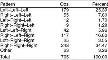
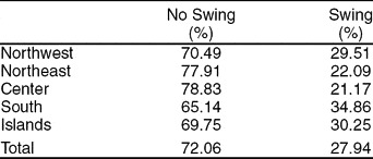
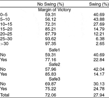
Table 1 shows that, in 25% of the districts, the center-left coalition won all three elections, whereas the center-right always won in 34%. The remaining 40% swung at least once. Safe (nonswing) districts are particularly concentrated in the northeast and center of the country (see Table 2). The lagged margin of victory in absolute value (MV) is an obvious measure of the ex ante contestability of the district: for example, if a coalition won by 30 percentage points in the previous election, it would be very difficult for the other coalition to fight back and win the district the next time. By the same token, alternative measures of the safeness of a district could be MV being greater than 5 (Safe1) or greater than 10 (Safe2) percentage points. The distribution of the margin of victory in single-member districts—expressed in percentage points—is positively skewed. In about 29% of the districts, the lagged margin of victory was lower than 5, whereas in about 49%, it was lower than 10.
Patterns of Political Victory in Single-member Districts

Notes: Left stands for victory of the center-left coalition; Right stands for victory of the center-right coalition; Other means victory of at least one third-coalition candidate. The first, second, and third term in each pattern refer to the XIIth, XIIIth, and XIVth legislative term, respectively.
Swing Districts According to Geographic Location

Notes: Swing is equal to one if the winner belongs to a different coalition this the incumbent. ISTAT geographic classification. Legislative terms XIII and XIV; 1,410 districts.
All these measures, based on the lagged margin of victory, should be good predictors of the swinging probability of a district, but their correlation with the characteristics of the individual candidates could be biased when the incumbent runs for reelection. In this case, the lagged margin of victory would refer to an election run by the same politician, and thus partly depend on his/her skills. Furthermore, measures based on the lagged margin of victory are not available for the XII legislative term, because the majoritarian districts were first introduced in this term. To address both issues, we construct an additional measure of contestability using the district-specific vote shares of different parties in the European elections, held either in 1994 or in 1999. We consider as ideological (or loyal) voters those who supported the center-left (D) or center-right coalition (R) in the previous European election. These elections, in fact, were held under proportional representation to appoint the Italian representatives in the European Parliament. Their turnout rate has usually been lower than in national elections, because government decisions are not at stake. It is therefore plausible to assume that voters cast a more ideological vote in this type of electoral contest than in the general (political) elections. Our new measure of safety (Safe3) is equal to one if

This measure can be interpreted as the empirical counterpart of 1/λk in the theoretical model. Furthermore, it has the advantage of allowing us to identify changes in the degree of contestability of a district due to national variations in political alliances within each coalition. As discussed above, large modifications occurred twice: before the 1996 election, when the separatist party Lega Nord left the center-right coalition; and before the 2001 election, when the leftist party Rifondazione Comunista left the center-left coalition. These alliance breakdowns originated from the (narrow) incentive of the two small parties to keep up their (proportional) vote share and bargaining power, and involved decisions by the national leaders. Their impact on the political future of backbenchers and on the contestability of districts was hardly internalized, as suggested by the fact that after the crises some incumbents left the two small parties to join large coalition parties. As a result, the political decisions of the leaders of these small parties, which followed purely “proportionalistic” motivations, ended up affecting the destiny of the representatives of big parties in marginal districts.Footnote 11 Hence, these national shocks altered the degree of contestability of some districts in a way that can be interpreted as exogenous with respect to the characteristics of politicians previously elected in those districts.
Table 3 shows that all our measures of ex ante contestability are correlated with the ex post probability that a district swings from one coalition to the other. The probability of swinging is always higher when our safeness indicators are equal to zero, and the differences are statistically significant either at the 1% level (Safe1 and Safe2) or at the 5% level (Safe3). The probability of swinging also increases with the lagged margin of victory.
Swing Districts According to the Lagged Margin of Victory

Notes: Swing is equal to one if the winner belongs to a different coalition with respect to the incumbent. Margin of victory is the lagged margin of victory in the single-member district. Safe1 is equal to one if the lagged margin is greater than 5 percentage points. Safe2 is equal to one if the lagged margin is greater than 10 percentage points. Safe3 is equal to one if (1−L−R)/|L−R|<1, where L (R) captures the expected share of voters for the center-left (center-right) coalition, estimated by means of ideological votes at the previous European elections. Legislative terms XIII and XIV; 1,410 districts.
Measuring Valence
The above measures of political competition represent our treatment of interest. We want to evaluate whether increasing the intensity of this treatment affects the patterns of political selection. In other words, we want to assess whether political parties allocate candidates with different (ex ante) valence according to the degree of contestability of each district. In line with Krasno and Green (Reference Krasno and Green1988), we think of quality (or valence) as something that exists in advance of and separate from other aspects of the electoral campaign. In particular, we measure valence as (i) years of schooling, (ii) previous market income, and (iii) past experience in local governments. The rationale for each measure is simple. Years of schooling capture the acquisition of formal human capital and skills.Footnote 12 Preelection income—controlling for the previous occupation—is a measure of market success and ability. The use of administrative experience is linked to the idea that lower-level elections can be used by high-quality politicians to build reputation and by voters to screen better candidates. Previous empirical studies have usually used lower-level electoral experience as a proxy for valence (see Jacobson Reference Jacobson1989; Shugart, Valdini, and Suominen Reference Shugart, Valdini and Suominen2005).Footnote 13
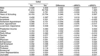
Table 4 summarizes the preelection characteristics of the politicians in our sample, according to the contestability of the districts where they were elected (as captured by the indicator Safe2). On average, candidates allocated to nonsafe districts are more educated, have lower parliament or government experience but greater local government experience, and declare higher preelection incomes. Physicians tend to run in more contestable districts. Party officers, in contrast, are allocated to safer districts.
Ex Ante Characteristics of the Members of Parliament

Notes: Safe2 is equal to one if the lagged margin of victory is greater than 10 percentage points. −diff95% and +diff95% represent the lower and upper bound of the 95% confidence interval of Difference, respectively. All variables are dummies, except Age, Years of Schooling, and Preelection Income (in million of euros, 2004 prices). Freshman means that the previous parliamentary tenure is zero. Parliament Appointment captures whether the politician has previously been president or vice president of the parliament, or of a single committee. Government Appointment captures whether the politician has previously been minister or vice minister. Local Government Experience stands for previous institutional experience at the local level (e.g., mayor). Preelection income is the total taxable income in the year before election (freshmen only). Job dummies refer to the preelection occupation and the omitted category includes blue collars and students. Legislative terms XIII and XIV; 1,307 observations.
Table 5 instead summarizes information on the ex post behavior and appointments of the members of parliament; Politicians elected in contestable districts tend to work harder in parliament, that is, they display a lower absenteeism rate in electronic votes, both overall and at the end of the legislative term.Footnote 14 It is worth noticing that politicians elected in contestable districts have a higher probability of entering the government (if their coalition wins the general election), although they have lower previous government experience than politicians running in safe districts (see again Table 4). This is consistent with the view that candidates in contestable districts are more skilled, and are therefore rewarded for winning tougher races.
Absences and Appointments of the Members of Parliament

Notes: Safe2 is equal to one if the lagged margin of victory is greater than 10 percentage points. −diff95% and +diff95% represent the lower and upper bound of the 95% confidence interval of Difference, respectively. Absenteeism Rate is the percentage of votes missed without any legitimate reason. Future Parliament Appointment captures whether the politician becomes president or vice president of the parliament, or of a single committee, after the election. Future Government Appointment captures whether the politician becomes minister or vice minister after the election. Legislative terms XIII and XIV; 1,307 observations.
THE IMPACT OF POLITICAL COMPETITION ON VALENCE
To evaluate whether any predetermined characteristic (X ijt) of politician i in district j at time t is associated with the degree of contestability of the district where he/she is elected (C ijt), we implement the following set of regressions (depending on the measure used to capture contestability):

where regional dummies γj control for geographical factors, δt for time fixed effects, the dummy URB j captures whether the electoral district belongs to an urban or rural area, and the error terms ηijt are clustered at the individual level. When C ijt is a dummy, we estimate a Probit model; when it is continuous, we use OLS. These estimations can be seen as a direct test of the main empirical prediction of our model, which suggests that high-quality candidates (defined on the basis of the ex ante observable characteristics that we use as proxies for valence) are more likely to run (and then to be elected) in contestable districts (see Proposition 2). The inclusion of the urban dummy and region fixed effects aims at removing the endogeneity problem due to (unobservable) local factors that might be correlated with both political selection and the degree of contestability.Footnote 15
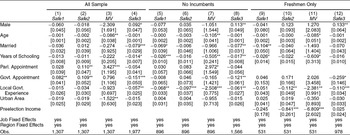
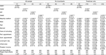
Estimation results are reported in Table 6. To control for the additional endogeneity problem arising from the spurious association between C ijt and X ijt, which arises when C ijt is based on the lagged margin of victory and is thus partly affected by the skills of the incumbent who is running for reelection, we also restrict the sample to nonincumbents only.Footnote 16 To evaluate the effect of preelection income, we further restrict the sample to freshmen, for whom preelection income refers to private activity and can thus be interpreted as market skills (controlling for occupation). For these three samples (all, no incumbents, and freshmen only), we estimate equation (7) using our four measures of political competition: the three measures based on the lagged margin of victory (Safe1, Safe2, and MV), available for terms XIII and XIV; and the measure based on the European elections (Safe3), available for the terms XII, XIII, and XIV. This is why the sample size of the estimate on Safe3 is always larger in the three (sub)samples.
The Impact of Political Competition on Political Selection

Notes: If Safe1, Safe2, or Safe3 as dependent variable: Probit estimation (marginal effects reported). If MV as dependent variable: OLS estimation. MV is the lagged margin of victory in the single-member district (available for legislative terms XIII and XIV). Safe1 is equal to one if MV is greater than 5 percentage points. Safe2 is equal to one if MV is greater than 10 percentage points. Safe3 is equal to one if (1−L−R)/|L−R| < 1, where L (R) captures the expected share of voters for the center-left (center-right) coalition, estimated by means of ideological votes at the European elections (available for legislative terms XII, XIII, and XIV). Urban area is a dummy capturing whether the electoral district belongs to an urban or rural area. Job fixed effects refer to the preelection occupation (see Table 4). Region fixed effects refer to ISTAT geographic classification (see Table 2). Robust standard errors clustered at the individual level in brackets. Significance at the 10% level is represented by *, at the 5% level by **, and at the 1% level by ***.
The results show that more years of schooling, past local government experience, and higher preelection income increase the probability of running for election in a contestable (nonsafe) district. In other words, the harsher is political competition, the higher is the probability that political parties rely on high-valence candidates. These are defined as politicians with higher educational attainments or private income—both proxies for market skills—or politicians who proved their political ability in subsequent rounds of local elections, which can be seen as “filters” for politicians' quality in a federal system (see Cooter Reference Cooter2002; Myerson Reference Myerson2006). The results are robust to the use of different contestability measures. We interpret this evidence as a validation of Proposition 2 in our model.Footnote 17
From a quantitative point of view, the estimates in Table 6, using for example the Safe1 indicator in the subsample without incumbents, suggest that two more years of schooling—equal to one standard deviation—increase the probability of running in a contestable district by 5.2 percentage points (i.e., by about 7% with respect to the average). Similarly, past administrative experience lowers the probability of running in a safe district by 6.8 percentage points (i.e., by 9%). Looking at the subsample of freshmen, even if we control for previous job fixed effects, preelection income has a negative impact on the probability of running in safe districts for two out of the four indicators. In particular, if we look at Safe2, an increase in preelection income equal to one standard deviation (421,000 euros) reduces the probability of running in a safe district by 35.4 percentage points (i.e., by 41%). An income increase of 100,000 euros would still produce a sizable effect, equal to 8.4 percentage points.Footnote 18
CONVERGENCE OF POLITICIANS' ATTRIBUTES IN CLOSE RACES
In the previous section, we showed that good politicians are more likely to run (and hence to be elected) in contestable districts, as predicted by Proposition 2 in our model. But is this allocation strategy common to both political coalitions? Is there any difference in political selection between the center-right and center-left? To shed light on this (complementary) point, we proceed in two steps. First, we look at any statistically significant difference in the observable characteristics of center-right versus center-left members of parliament. Second, we evaluate whether these differences (if any) survive in close elections, by implementing a regression discontinuity design (RDD) on the margin of victory of one coalition over the other, in the spirit of Lee (Reference Lee2008). So far, the latter identification strategy has been used to estimate the impact of political parties on policy outcomes [see Ferreira and Gyourko (Reference Ferreira and Gyourko2009) for the United States; and Pettersson-Lidbom (Reference Pettersson-Lidbom2008), for Sweden]. We instead use it to test for the presence of intrinsic differences in the political selection decisions of the main political coalitions in Italy. In fact, if there was any intrinsic difference in the political personnel of the two coalitions, this should remain even in close elections, that is, when the victory of one coalition over the other is due to random events.
Formally, we calculate the margin of victory of the center-right coalition (MVR) in each district: this measure is positive (negative) in all districts won by the center-right (center-left) coalition. We then look at the predetermined characteristics X ijt of politician i elected in district j at time t (with a particular attention to our valence indicators) and fit a p-order polynomial in MVR on either side of the threshold MVR = 0, at which the electoral result sharply changes in favor of the center-right:

where D ijt = 1[MVR ijt > 0] and the error terms ψijt are clustered at the individual level. The parameter τ identifies the effect of interest: that is, whether politicians elected in close races (i.e., at MVR = 0) are intrinsically different in their observable characteristics according to the political coalition they belong to. The underlying assumption of this identification strategy is that electoral outcomes depend on both predictable elements (such as candidates' skills and valence) and random chance (such rain on election day), which, however, becomes crucial only for close electoral races. It is important to notice that in this analysis we are using the actual (instead of the lagged) margin of victory, so that the victory of one coalition over the other at MVR = 0 represents a random event. As a result, a significant jump in politicians' attributes would show up only if the two coalitions followed alternative (nonsymmetric) allocation strategies in close electoral races.
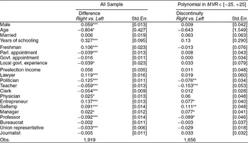
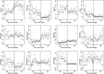
The first panel of Table 7 reports the results for the whole sample of members of parliament. On the average, left-wing politicians are older, are less educated, and feature a longer parliament tenure and more local government experience. The right-wing coalition recruits more entrepreneurs, self-employed previous, and lawyers; the left-wing coalition selects more professional politicians, teachers, college professors, union representatives, and females.
Partisan Differences in Political Selection, All versus Close Races

Notes: Difference is the difference between the average characteristics of center-right politicians and the average characteristics of center-left politicians in all districts. Discontinuity is the estimated difference for close races, i.e., the discontinuity at zero of a split 3rd-order polynomial in the margin of victory of the center-right coalition (MVR), fitted over the interval MVR ∈[−25, +25]. Standard errors are in brackets. Significance at the 10% level is represented by *, at the 5% level by **, and at the 1% level by ***. All dependent variables are dummies, except Age, Years of Schooling, and Preelection Income (in million of euros, 2004 prices). Freshman means that the previous parliamentary tenure is zero. Parliament Appointment captures whether the politician has previously been president or vice president of the parliament, or of a single committee. Government Appointment captures whether the politician has previously been minister or vice minister. Local Government Experience stands for previous institutional experience at the local level (e.g., mayor). Preelection Income is the total taxable income in the year before election (freshmen only). Job dummies refer to the preelection occupation and the omitted category includes blue collars and students. Legislative terms XII, XIII, and XIV.
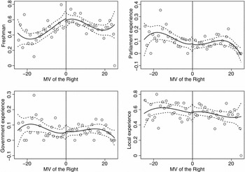
The two main political coalitions thus show very different patterns of political selection. Yet the RDD evidence shows that they both converge to the same (high-valence) type in close races. The second panel of Table 7 reports the estimated discontinuity at a zero margin of victory: there is no significant difference between center-right and center-left politicians in any demographic characteristic or previous market and political experience. In particular, education, parliament tenure, gender, and local government experience, despite being different in the whole sample, are perfectly balanced in close races.
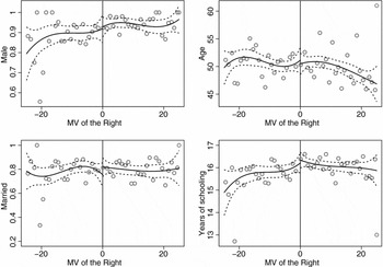
Figures 2 through 4 provide a graphical representation of the estimated polynomials and of the jumps at MVR = 0. These figures clearly show a pattern of convergence in the predetermined attributes (and valence) of political candidates. For instance, the center-left coalition has fewer candidates with high educational attainments, but allocates all of them to marginal districts, where the gap with the center-right coalition is thus filled; all candidates with lower education are instead allocated to safer districts. Only with respect to the previous occupations, where the two coalitions may be supply-constrained in certain characteristics, does the center-left select fewer entrepreneurs and self-employed previous, and the center-right fewer teachers and professional politicians. These intrinsic differences also remain in close electoral races (see Figure 4).
Convergence of Demographic Characteristics in Close Races

Convergence of Political Experience in Close Races

Convergence of Market Experience in Close Races

THE IMPACT OF POLITICAL COMPETITION ON EFFORT
To evaluate whether the degree of ex-ante contestability (C ijt) affects the in-office effort captured by the absenteeism rate (Y ijt) of politician i elected in district j at time t, we run the following regressions:

where X ijt are the predetermined individual characteristics, P ijt represent additional postelection characteristics affecting the absenteeism rate (e.g., belonging to the majority coalition or being appointed to a government position), γj and δt are regional and time fixed effects, the dummy URB j captures whether the electoral district belongs to an urban or rural area, and the error terms ϵijt are corrected for clustering at the individual level. The absenteeism rate is a measure of shirking or rent extraction, because it excludes absences with a legitimate reason; moreover, we control for political appointments that may reduce parliamentary attendance. In the subsample of freshmen, we also control for preelection income, which has been shown to be a good predictor of outside income and shirking in parliamentary activity (see Gagliarducci, Nannicini, and Naticchioni Reference Gagliarducci, Nannicini and Naticchioni2010).
By estimating the impact of ex ante political competition on the future performance of elected officials, we want to assess whether the positive effect of electoral competition on selection also leads to better political outcomes, that is, whether more skilled candidates perform better once in office. Table 8 reports the estimation results. As in Table 6 above, we estimate the baseline specification in three samples (all, no incumbents, and freshmen only) using four measures of political competition (with three of them available for terms XIII and XIV, and one of them—Safe3—available for terms XII, XIII, and XIV). The empirical evidence shows that politicians elected in contestable districts display a lower absenteeism rate in electronic parliamentary votes. If we look at the Safe1 indicator in the subsample without incumbents, for example, running in a contestable district reduces the ex post absences by 4.9 percentage points (i.e., by about 16% with respect to the average). The effects are always significant at the 1% or 5% level, irrespective of the contestability measure we use.Footnote 19
The Impact of Political Competition on the Absenteeism Rate

Notes: Dependent variable: absenteeism rate. OLS estimations. MV is the lagged margin of victory in the single-member district (available for legislative terms XIII and XIV). Safe1 is equal to one if MV is greater than 5 percentage points. Safe2 is equal to one if MV is greater than 10 percentage points. Safe3 is equal to one if (1−L−R)/|L−R|<1, where L (R) captures the expected share of voters for the center-left (center-right) coalition, estimated by means of ideological votes at the European elections (available for legislative terms XII, XIII, and XIV). Urban Area is a dummy capturing whether the electoral district belongs to an urban or rural area. Job fixed effects refer to the preelection occupation (see Table 4). Region fixed effects refer to ISTAT geographic classification (see Table 2). Robust standard errors clustered at the individual level in brackets. Significance at the 10% level is represented by *, at the 5% level by **, and at the 1% level by ***.
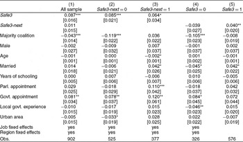
These findings may be driven by selection, but they may also have an alternative explanation: members of parliament facing tougher political competition might choose to exert more effort in order to gain reelection. To disentangle whether the higher productivity of politicians elected in contestable districts arises from the selection of better candidates or from different reelection incentives, we exploit the (exogenous) changes in national coalitions discussed above, which altered the degree of contestability of certain districts from one election to the next. In Table 9, Safe3 is constructed as before (see equation (6)), whereas Safe3-next uses the same method but refers to the next election (keeping into account the variations that occurred in the political alliances within coalitions). As outcome variable, we use the absenteeism rate during the last year of the legislative term, because at that time the new electoral coalitions are known and reelection incentives are probably at their maximum.
Political Competition and Absences in the Last Year of the Term

Notes: Dependent variable: absenteeism rate in the last year of the legislative term. OLS estimations. House of Representatives only. Safe3 is equal to one if (1−L−R)/|L−R| < 1, where L (R) captures the expected share of voters for the center-left (center-right) coalition, estimated by means of the votes at the previous European elections (available for legislative terms XII, XIII, and XIV). Safe3-next is calculated in the same way but keeping into account the variations in national political coalitions at the following election, in order to capture reelection incentives. Urban area is a dummy capturing whether the electoral district belongs to an urban or rural area. Job fixed effects refer to the preelection occupation (see Table 4). Region fixed effects refer to ISTAT geographic classification (see Table 2). Robust standard errors clustered at the individual level in brackets. Significance at the 10% level is represented by *, at the 5% level by **, and at the 1% level by ***.
Column (1) shows that the effect of the ex ante contestability (Safe3) remains strong: even if we control for future reelection incentives (Safe3-next), good politicians—elected in contestable districts—reduce their absences by 8.7 percentage points (about 37% with respect to the last-year average). Columns (2) and (3) confirm this result: (bad) politicians elected in safe districts here more absences at the end of the legislative term, both when their district has turned contestable and when it has remained safe. Selection hence matters. Similarly, in columns (3) and (4), we look at the impact of the future contestability of the district on last-year absences, controlling for the ex ante contestability. As expected from the result in column (1), incentives are less relevant. Yet there is still some evidence of an additional accountability effect for low-quality politicians. In fact, if a safe district turns contestable, (bad) politicians tend to exert more effort (by 4 percentage points, about 17%). But the opposite does not hold: (good) politicians elected in contestable districts show high productivity even when their districts turn safe.
Finally, note that the change in the degree of contestability for the districts that from safe turned contestable, or vice versa, is indeed large in our data, especially because of the coalition adjustments that took place between the 1996 election (when the center-right ran without “Lega Nord” and the center-left with “Rifondazione Comunista”) and the 2001 election (when the center-right ran with “Lega Nord” and the center-left without “Rifondazione Comunista”). As a result of this reshuffling, in the districts that from contestable turned safe, the average margin of victory doubled (from 7% to 14%); whereas in the districts that from safe turned contestable, it was almost halved (from 15% to 8%). In the other districts, the variation in the average margin of victory was much lower: from 11% to 10% in districts that remained contestable; from 15% to 13% in districts that remained safe. These variations thus provide enough power to our test so that the above results can be interpreted as a way to disentangle the selection from the incentive channel of the impact of political competition on effort in parliamentary work.
CONCLUSION
In this paper, we address a recurring question in political science and political economy: is electoral competition as quality-enhancing as economic competition? We provide a positive answer and suggest a possible channel: the selection of high-quality candidates by political parties that want to attract unaligned voters.
Our theoretical model provides a crucial role for the parties in selecting and allocating politicians to the different electoral districts. Hence, we disregard self-selection by individual politicians and concentrate on the effect of political competition on party selection. Our ideological parties select party loyalists and experts—who are highly valued by the swing voters, but costly for the parties—and allocate them into districts in an attempt to increase their probability of winning the election. Political competition pushes political parties to increase the share of (high-valence) experts, and to allocate them to the most contestable districts.
The ground field to test this prediction is the Italian majoritarian political system between 1994 and 2006. And the empirical evidence supports our prediction. Ex ante valence—as measured by years of schooling, previous market income, and local government experience—increases the probability of running in a contestable district. Evidence from a regression discontinuity design shows that, despite being different on average, the personal attributes of the politicians of the two major coalitions converge to high-valence levels in close electoral races. Politicians elected in nonsafe districts also have a better level of ex post quality, as measured by their absenteeism rate in parliament. This higher effort is driven more by the selection of better politicians than by reelection incentives. Accountability does, however, play an additional role, at least for low-quality candidates: if a safe district turns contestable, politicians tend to exert more effort. Yet high-quality politicians elected in contestable districts do not reduce their ex post productivity even when their districts become safe.
Our results have normative implications. They encourage the adoption of institutions and policies aimed at enhancing both political competition and voters' information on the quality of individual candidates. For example, in a majoritarian system, the amount of ex ante contestability could be increased by “optimal” gerrymandering that evens out the relative shares of the main parties' ideological voters across electoral districts. We leave the study of these implications to future research.
APPENDIX
Formal Version of Proposition 1
Before a formal version of Proposition 1 is provided, it is convenient to introduce some definitions. Define ΛD, party-D allocation of experts, as the union of the district intervals ΛiD = [λIi, λIIi] where party D allocates its experts, ΛD = ∪iΛiD, and analogously ΛR for party R. Moreover, define z = μD − μR ∈ [−1, 1], as the difference in the share of experts between party D and R.
Proposition 1. Parties allocate experts in district intervals as follows.Footnote 20
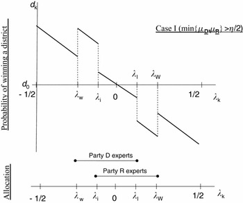
(I) For η/2 ≤ min {μD, μR}, party-D allocation of experts ΛD includes ΛiD = [λIi, λ IIi] with λIi < λw and λIIi > λΞ; and party-R allocation ΛR includes ΛiR = [λIi, λIIi] with λIi < λϵ and λIIi > λW. For η/2 < min {μD, μR}, parties have equal probability of winning the elections, ΠD = ΠR = 1/2; for μD > η/2 = μR, parties probability of winning the elections are ΠD = 1/2 + ψ[(1 − λC)/λC]η/4 and ΠR = 1− ΠD; and analogously for μR > η/2 = μD. See Figure 5.
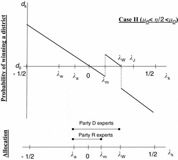
(II) For μD > η/2 > μR, party-D allocation of experts is ΛD = [λa, λW], such that G(λW) − G(λa) = μD, and party-R allocation is ΛR = [λj, λm], such that G(λm) − G(λa) = μR and λj = max {λa, λw}. Parties' probabilities of winning the elections are ΠD = 1/2 + [(1 − λC)/2λC]ψz and ΠR = 1 − ΠD. And analogously for μR > η/2 > μD. See Figure 6.
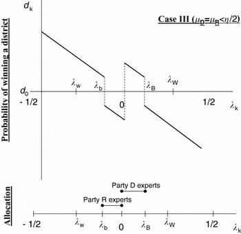
(III) For μD = μR = μ ≤ η/2, party-D allocation of experts is ΛD = [λ0, λB], such that G(λB) = 1/2 + μ, and party-R allocation is ΛR = [λb, λ0], such that G(λb) = 1/2 − μ. Parties have equal probability of winning the elections, ΠD = ΠR = 1/2. See Figure 7.
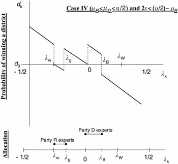
(IV) For μR < μD < η/2 and z < (η/2 − μR)/2, party-D allocation of experts is ΛD = [λ0, λB], such that G(λB) = 1/2 + μD, and party-R allocation is ΛR = [λw, λg], such that G(λg) − G(λw) = μR. Parties' probabilities of winning the elections are ΠD = 1/2 + [(1 − λC)/λC]ψz and ΠR = 1 − ΠD. And analogously for μD < μR < η/2 and z < (η/2 − μD)/2. See Figure 8.
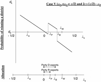
(V) For μR < μD ≤ η/2 and z ≥ (η/2 − μR)/2, party-D allocation of experts is ΛD = [λ0, λB], such that G(λB) = 1/2 + μD, and party-R allocation is ΛR = [λ0, λc], such that G(λc) = 1/2 + μR. Parties' probabilities of winning the elections are ΠD = 1/2 + [(1 − λC)/2λC]ψ(η/2 − μR) and ΠR = 1 − ΠD. And analogously for μD < μR ≤ η/2 and z ≥ (η/2 − μR)/2. See Figure 9.
Equilibrium Allocation Game, Case I

Equilibrium Allocation Game, Case II

Equilibrium Allocation Game, Case III

Equilibrium Allocation Game, Case IV

Equilibrium Allocation Game, Case V
Notes: When the asymmetry is larger, because party D has several more experts than party R (i.e., z is large), although neither party spans the crucial districts, party D strategy remains unchanged, and experts are thus sent to [λ0, λB]. In an attempt to limit party D electoral chances, also party R will allocate its few experts to the right of the more competitive districts, as shown in the figure. The resulting probability of winning the election for party D is ΠD = 1/2+[1−λC)/2λC]ψ .

Proof. See the supplemental online Appendix at http://www.journals.cambridge.org/psr2011002





Comments
No Comments have been published for this article.