Introduction
A circularly polarized (CP) antenna has the benefit of combating the multipath propagation [Reference Le1], accommodating the object movement [Reference Jiang and Werner2], and increasing the channel capacity rather than the linear polarization [Reference Ullah, Al-Hasan, Koziel and Mabrouk3]. Many methods were proposed to obtain a CP patch antenna, such as using a single feedline with radiator perturbation [Reference Abed, Singh and Jawad4, Reference Saraswat, Kumar and Harish5], helical shape antenna [Reference Yao and Georgakopoulos6, Reference Li, Wang, Hu and Lin7], and two orthogonal elements [Reference Tang, Li, Wang, Hu and Ziolkowski8, Reference Yan, Sharif and Ouyang9]. In the two orthogonal feedlines method, a 90° delay circuit is essential to ensure the generation of circular polarization. Conversely, in the single feedline approach, a perturbation radiator is employed to manipulate the surface current flow on the radiator, achieving circular polarization. It is known that two orthogonal feedline techniques can provide wider axial ratio bandwidth (ARBw) than the single feedline because, with the right composition, the two feedlines can create two oscillations on axial ratio, thus widening the ARBw [Reference Jiang and Werner2, Reference Wu, Zhang and Zhu10]. However, many single feedline techniques have been conducted to obtain a wide ARBw using parasitic elements and radiator perturbation [Reference Santosa, Sumantyo, Gao and Ito11–Reference Rai, Sigroha, Tyagi, Das and Sharma15].
In most cases, integrating an antenna and filter is primarily performed to add the selectivity function to an antenna [Reference Suryarajitha, Jawale, Basavarajappa, Sigmarsson, Panigrahi and Kartikeyan16–Reference Xu, Xing, Shi, Jiang, Li, Wang and Wu19]. However, some studies have proposed filtering antennas with an added circular polarization feature, achieved through two orthogonal feedlines [Reference Jiang and Werner2, Reference Wu, Zhang and Zhu10, Reference Wu, Zhang and Zhu20], circular disk radiator [Reference Qin, Han, Zhang, Mao and Zhu21], truncated radiators, and cross slots [Reference Dong, Gao, Luo, Wen, CX, SW, Li, Wei, Wen, Geng and Cheng22–Reference Zhou, Pan, Cheng, Yang, Li and Huang25]. These methods typically involve a two-step design process, with the first step focusing on the filtering structure design and the second step on the generating circular polarization design. The most common method for designing a filtering antenna is by replacing the last stage resonator of the filter with a radiator [Reference Qin, Han, Zhang, Mao and Zhu21, Reference Cheng and Li26]. Several studies have explored these types of filtering antennas with circular polarization using two orthogonal feedlines [Reference Jiang and Werner2, Reference Wu, Zhang and Zhu10, Reference Wu, Zhang and Zhu20, Reference Wang, Zhang, Ye and Liu27]. However, all CP filtering antennas that employ two feedlines were designed with both a filtering structure and an added delay circuit, making the design process more complicated due to the requirement of a two-step design approach. Moreover, employing two orthogonal feedlines further complicates the design of array antennas.
Recently, a new method of combining an integrated antenna and filter component has resulted in a filtering antenna with a linear or circular polarization [Reference Cahyasiwi, Zulkifli and Rahardjo28–Reference Cahyasiwi, Roza, Mujirudin, Nashuha, Zulkifli and Rahardjo31]. This approach enables the simultaneous achievement of selectivity and polarization features through an integrated step design. By applying this method, a second-order CP filtering antenna is designed using a single feedline [Reference Cahyasiwi, Zulkifli and Rahardjo28]. However, its ARBw remains narrow even when designed with double-layer substrates. Here, we propose a novel third-order filtering antenna design that integrates circular polarization generation using only a single feedline. In contrast to previous work [Reference Cahyasiwi, Zulkifli and Rahardjo28], which employed lower-order designs, our approach enhances selectivity, impedance, and ARBw by leveraging the inherent benefits of a higher-order filtering circuit. By codesigning the filtering circuit and the polarization generator, we eliminate the need for an additional delay circuit, thereby simplifying the overall architecture. The proposed antenna is optimized for operation at 4.65 GHz, well-suited for C-band wireless systems where polarization robustness and inherent out-of-band suppression are required. Potential applications include short- to medium-range radar systems, microwave point-to-point communication links, and RF energy harvesting, where compactness, single-feed simplicity, and integrated filtering characteristics offer practical advantages.
Antenna design
Antenna configuration
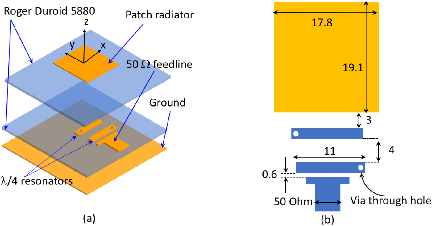
As shown in Fig. 1(a) and (b), the antenna consists of a rectangular radiator measuring 17.8 mm × 19.10 mm printed on the upper substrate, coupled with two λ/4 resonators with a thickness of 2.4 and 11 mm in length lying on the lower substrate. There is a 3 mm gap between the rectangular radiator and the second λ/4 resonator, which not only provides coupling between them but also a 90° phase delay. There is a 4 mm gap between the two λ/4 resonators. A 50-ohm feedline is coupled to the first resonator with a gap of 0.6 mm. The extraction of the radiator and the resonator is conducted as in Ref. [Reference Cahyasiwi, Zulkifli and Rahardjo28], where the length of the radiator (L p) determined the radiator resonance frequency, while the length (P k), thickness of the resonator, and the position of a via through hole determined the resonator’s resonance frequency [Reference Cahyasiwi, Zulkifli and Rahardjo28, Reference Cahyasiwi, Zulkifli and Rahardjo29, Reference Cahyasiwi, Roza, Mujirudin, Nashuha, Zulkifli and Rahardjo31]. The two λ/4 resonators with a via through-hole not only serve to shape the gain for enhanced selectivity but also act as a mechanism to induce second-mode polarization in the radiator.
The configuration of the proposed CP filtering antenna (a) 3-dimensional view with transparent substrates and (b) top view with transparent substrates and dimensions (all units in mm).

Figure 1 Long description
The image consists of two parts. The first part, labeled as (a), shows a three-dimensional view of a CP filtering antenna. It includes multiple layers: the top layer is labeled 'Patch radiator,' followed by a '50 ohm feedline,' and a 'Ground' layer. Below these, there are 'lambda over 4 resonators.' The substrate material is indicated as 'Roger Duroid 5880.' Arrows point to each labeled component, showing their positions within the layered structure. The second part, labeled as (b), presents a top view of the antenna with dimensions marked in millimeters. The rectangular patch radiator measures 17.8 millimeters by 19.1 millimeters. Below the patch, there is a gap of 3 millimeters leading to a section labeled '11 millimeters,' which is part of the resonator structure. A 'Via through hole' is shown, connecting to a '50 ohm' section, with a thickness of 0.6 millimeters. The diagram provides a detailed view of the antenna's configuration and dimensions.
Equivalent circuit and design procedure
The equivalent circuit network of the CP filtering antenna is shown in Fig. 2, where two series resonators are described as L 1, C 1, and L 2, C 2 for the first and second resonators, respectively. The short circuit holes on the left and right arms of the first and second resonators lead to a horizontal current flow along the transmission line. Upon reaching the rectangular radiator (L A, C A, and R A), there arises an interaction between two electric field vectors that are orthogonal to each other. The CP filtering antenna is obtained when the two vectors' magnitudes are balanced, and the phase delay is ±90°. The space between the second resonators and the radiator (CB) functions both as the delay circuit and coupling. The radiator’s dimensions are not square, dissimilar to the orthogonal feedline methods. W p should be marginally shorter than L p to balance the magnitudes of the orthogonal vectors. The space between the resonator (Gap 1) affects the IBw, selectivity response, and axial ratio at the center and lower frequency.
Equivalent circuit and design concept.

Figure 2 Long description
The diagram illustrates the equivalent circuit network of a CP filtering antenna. At the top left, a rectangular radiator labeled 'Radiator' is connected to a section marked 'Delay' with a component labeled 'CB'. Below this, a gap labeled 'Gap1' is shown, followed by a section labeled 'port' with components 'Lc' and 'Zc'. To the right, a series of resonators and coupling elements are depicted. The top section, enclosed in a blue dashed box, includes a resonator with components 'RA', 'LA' and 'CA', labeled 'Coupling and phase delay 90 degrees'. Below, a green shaded area contains two resonators. The upper resonator is labeled 'L2' and 'C2' and the lower one is labeled 'L1' and 'C1', both marked as 'Coupling'. A red arrow points from the 'Delay' section to the resonators, indicating the flow of interaction. At the bottom, a section labeled 'port' includes components 'Z0', 'Zc' and 'Vg'. The diagram shows the arrangement and connection of these elements, illustrating the design concept of the CP filtering antenna.
The concept of the orthogonal resonators refers to the fundamental equation of the electromagnetic wave polarization vector in Eq. (1). This equation explains that the polarization vector is the resultant of the superposition of two distinct polarization vectors, each oriented orthogonally in the θ and φ directions. The production of circular polarization is subject to the equal magnitude of the θ and φ vectors as in Eq. (2) and a phase difference ( ${\delta _{\text{L}}})$ of approximately ± 90° between these vectors. Consequently, the orthogonality of these vectors can be established through the integration of two resonators featuring orthogonal current orientations. In the context of this study, this is exemplified by the utilization of the two quarter-wavelength resonators in the θ direction as the first resonator, and a rectangular radiator in the φ direction as the second resonator.
 \begin{equation}\overline E \, = \,{E_\theta }cos{\text{(}}\omega t{\text{)}}\widehat \theta \, + \,{E_\Phi }\,cos{\text{(}}\omega {\text{t}}\,{\text{ + }}\,{{{\delta }}_{\text{L}}}{\text{)}}\widehat \Phi \end{equation}
 \begin{equation}\left| {{E_\theta }} \right|\, = \,\left| {{E_\Phi }} \right|\end{equation}
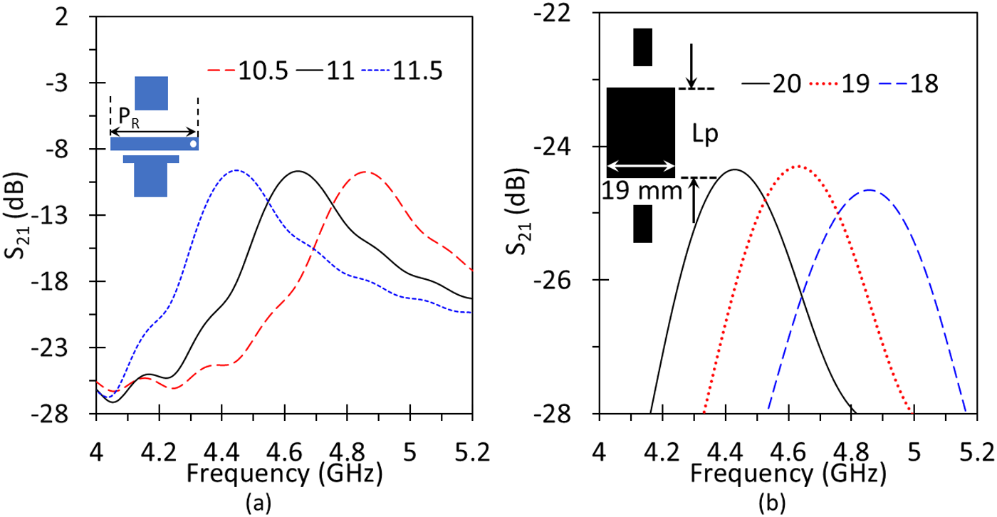
The orthogonality can be observed from the surface currents of both resonators, as seen in Fig. 3(a), where the horizontal surface current of two λ/4 resonators flows reversely along the x-direction from the open circuit to the short circuit (via through hole). On the contrary, Fig. 3(b) depicts the radiator surface current that flows along the vertical position or y direction when fed from the lower side of its length. Both circuits must operate at an identical frequency. The integration result of the two vector directions is shown on the radiator, forming the right-hand circular polarization (RHCP) as depicted in Fig. 3(c). The length of the λ/4 resonator (P R) and the position of the via through-hole determine its resonant frequency as shown in Fig. 4(a). Two λ/4 resonators are used to create the two minimal axial ratios and multiple resonants in S 11. The addition of the resonator in filter design also aims to increase its selectivity. The resonant frequency of the rectangular radiator shown in Fig. 4(b), is affected essentially by its length (L p) while its width (W p) can be adjusted for balancing the magnitude of the two orthogonal vectors.
Concept of orthogonal resonators from the surface current of the (a) λ/4 resonator as the first resonator, (b) radiator as the second resonator, and (c) the interaction of the two vectors on the filtering antenna’s radiator.

Figure 3 Long description
The composite figure contains three quiver vector-field plots labeled (a), (b) and (c), each displaying surface current density across a resonator geometry. Arrows indicate the local direction of current flow and the color of each arrow encodes the magnitude of the surface current density, measured in A/m. Each plot includes a vertical color bar on the right side. In plot (a), the color bar ranges from approximately 0 to 310 A/m. The spatial axes are labeled x and y, with the x-axis oriented horizontally and the y-axis oriented vertically. A horizontal red line is visible along the bottom edge of the plot area. The arrows in plot (a) are arranged in two vertically oriented groups, with two large bold arrows pointing in opposite vertical directions, one upward and one downward, placed centrally in the plot. The surrounding smaller arrows follow a broadly vertical alignment. In plot (b), the color bar ranges from approximately 0 to 95 A/m. The x and y axes are present with the same orientation. A horizontal red line appears along the bottom edge. Two horizontal groups of arrows are visible, with bold arrows pointing in opposite horizontal directions, one to the right and one to the left, placed at mid-height in the plot. Surrounding arrows are broadly horizontally oriented. In plot (c), the color bar ranges from approximately 0 to 130 A/m. The x and y axes are present. A horizontal red line appears at the bottom edge. A circular outline is visible in the upper portion of the plot area. The arrows in this panel show a combined pattern, with vertical arrows in the lower portion and a circulating arrow arrangement visible near the circular outline region. The red line present at the bottom of all three plots occupies the full horizontal width of each plot area.
The resonance frequency simulation of (a) the radiator as a function of the variation in its length (L p) with a fixed width (W p = 19 mm) and (b) the resonator as a function of the variation in its length (P R). All dimensional units are in millimeters.

Figure 4 Long description
The image A showing a line graph with the vertical axis label “S subscript 11 (dB)” and the horizontal axis label “frequency (GHz)”. The horizontal axis range is 4 to 5.2. The vertical axis range is negative 28 to 2. A legend shows three series labels: “10.5”, “11” and “11.5”. The plotted curves show local minima near frequency 4.0 to 4.1 at about negative 27 to negative 28. The “11” series has a peak near (4.6, about negative 8). The “10.5” series has a peak near (4.8, about negative 8). The “11.5” series has a peak near (4.7, about negative 10). The label “(a)” appears below the plot. The image B showing a line graph with the vertical axis label “S subscript 21 (dB)” and the horizontal axis label “frequency (GHz)”. The horizontal axis range is 4 to 5.2. The vertical axis range is negative 28 to negative 22. A legend shows three series labels: “20”, “19” and “18”. The plotted curves show peaks near frequency 4.5 to 5.0 at about negative 24. The “20” series has a peak near (4.5, about negative 24). The “19” series has a peak near (4.6, about negative 24). The “18” series has a peak near (4.9, about negative 24). The label “(b)” appears below the plot. A small inset diagram appears near the upper left of the plot area with the text “L subscript p” and “19 mm”.
After obtaining the frequencies of both resonators, the integration is carried out using a single port. The determination of the gap distance between the λ/4 resonator and the port (L c) is made with the consideration of being sufficiently close to provide a strong current to the feedline, thus setting the distance at 0.6 mm. So, there are four variables left to obtain the CP characteristics which are the size of the radiator, the space between the λ/4 resonators and the space between the radiator and λ/4 resonator. From the previous study, the space between the radiator and resonator functions both as the delay and matching circuit [Reference Cahyasiwi, Zulkifli and Rahardjo28], then in this design, we start with 3.6 mm to iterate the response. The optimization goal was to achieve the axial ratio less than 3 dB over the bandwidth and IBw of −10 dB using the variations of W p, L p, CB, and Gap 1.
Analysis of coupled quarter-wavelength resonators
In Ref [Reference Suryarajitha, Jawale, Basavarajappa, Sigmarsson, Panigrahi and Kartikeyan16], a single quarter-wavelength resonator was employed to implement the filtering structure for the antenna, which provides acceptable filtering performance. However, the single-resonator approach inherently limits the operational bandwidth and selectivity. In this work, we extend the design by employing two coupled quarter-wavelength resonators as shown in Fig. 2. It is well established that a single quarter wavelength resonator typically yields a first-order response with a relatively narrow bandwidth and a moderate roll-off. In contrast, when two quarter-wavelength resonators are coupled together, a higher-order response is achieved. This coupled configuration introduces additional degrees of freedom, allowing for enhanced selectivity, a broader operational bandwidth, and steeper attenuation slopes in the transition bands. The coupling also enables tailoring the resonant modes, leading to improved out-of-band rejection and a more flexible design for achieving the desired filter characteristics.
To explain the presence of a higher-order mode in our proposed filter design, the coupled mode theory (CMT) framework is used to derive analytical expressions for the transmission S 21 and reflection S 11 coefficients. In this model, we consider two resonators (assumed identical) having a resonant angular frequency  $A = {{{\omega }}_0}$ and are coupled to ports 1 and 2 with an external coupling rate
 $\sqrt {{\gamma _e}} $. They are also mutually coupled with a coupling coefficient
 $\kappa $. Assuming negligible intrinsic loss, the time‐domain dynamics (with a harmonic excitation
 ${s_{1 + }}\left( t \right) = {s_{1 + }}{e^{ - j\omega t}}$) lead to the steady‐state equations for the resonator amplitudes
 ${a_1}$ and
 ${a_2}$ written as [Reference Haus and Weiping32, Reference Fan, Suh and Joannopoulos33],
 \begin{equation}{a_2} = - \frac{{j\kappa }}{{ - j\left( {\omega - {\omega _0}} \right) + \frac{{{\gamma _e}}}{2}}}{a_1},{\text{ }}\end{equation}
 \begin{equation}{a_1} = {\text{ }}\frac{{\sqrt {{\gamma _e}} {s_{1 + }}\left[ { - j\left( {\omega - {\omega _0}} \right) + \frac{{{\gamma _e}}}{2}} \right]}}{{{{\left[ { - j\left( {\omega - {\omega _0}} \right) + \frac{{{\gamma _e}}}{2}} \right]}^2} + {\kappa ^2}}}{a_1}.{\text{ }}\end{equation}
The output at port 2 is given by the standard input–output relation 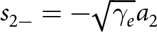 ${s_{2 - }} = - \sqrt {{\gamma _e}} {a_2}$, which gives us,
 \begin{equation}{s_{2 - }} = \sqrt {{\gamma _e}} \frac{{j\kappa }}{{ - j\left( {\omega - {\omega _0}} \right) + \frac{{{\gamma _e}}}{2}}}{a_1}.{\text{ }}\end{equation}
Substituting the expression for  ${a_1}$ we obtain
 \begin{equation}{s_{2 - }} = {\gamma _e}\frac{{j\kappa {s_{1 + }}}}{{{{\left[ { - j\left( {\omega - {\omega _0}} \right) + \frac{{{\gamma _e}}}{2}} \right]}^2} + {\kappa ^2}}}.{\text{ }}\end{equation}
Thus, we can derive the transmission coefficient as,
 \begin{equation}{S_{21}}\left( \omega \right) = \frac{{{s_{2 - }}}}{{{s_{1 + }}}} = \frac{{{\gamma _e}j\kappa }}{{{{\left[ { - j\left( {\omega - {\omega _0}} \right) + \frac{{{\gamma _e}}}{2}} \right]}^2} + {\kappa ^2}}}.{\text{ }}\end{equation}
Similarly, using the input–output relation at port 1,  ${s_{1 - }} = {s_{1 + }} - \sqrt {{\gamma _e}} {a_1}$, we obtain the reflection coefficient
 \begin{equation}{S_{11}}\left( \omega \right) = 1 - \frac{{{\gamma _e}\left[ { - j\left( {\omega - {\omega _0}} \right) + \frac{{{\gamma _e}}}{2}} \right]}}{{{{\left[ { - j\left( {\omega - {\omega _0}} \right) + \frac{{{\gamma _e}}}{2}} \right]}^2} + {\kappa ^2}}}.{\text{ }}\end{equation}
To confirm the above CMT model in our proposed filter design, we simulate a microstrip filter using two quarter-wavelength resonators in CST Microwave Studio. Details of the filter geometrical parameters can be found in Fig. 5, which illustrates the coupled quarter-wavelength resonators analysis based on the coupled-mode theory (CMT) model. Figure 5(a) illustrates the geometrical parameters of the microstrip filter utilizing two quarter-wavelength resonators. Figure 5(b) shows the simulation setup in CST. Figure 5(c) and 5(d) presents the comparison between simulation results and analytical calculation results using CMT for Fig. 5(c) transmission coefficient (S21) and Fig. 5(d) reflection coefficient (S11). Figure 5(a) and the simulation setup is shown in Fig. 5(b). Figure 5(c) and (d) shows the transmission and reflection coefficients obtained by using the simulation and the analytical calculation (Eqs. (7a) and (7b)). In our analytical model, we employed a resonant frequency f 0 = 4.65 GHz, an external coupling rate of  ${\gamma _e} = 1.7 \times {10^9}$ per port, and a resonator coupling coefficient
 $\kappa = 1.25 \times {10^9}$. The simulation results confirm that the two-resonator configuration achieves a broader bandwidth while maintaining improved selectivity, as evidenced by the enhanced transmission and reduced reflection over the frequency range of interest. The two coupled quarter-wavelength resonators yield a higher-order response with steeper roll-off compared to single-resonator designs, enabling better selectivity.
Coupled quarter-wavelength resonators analysis by the coupled-mode theory (CMT) model. (a) Geometrical parameters of the microstrip filter utilizing two quarter-wavelength resonators. (b) Simulation setup in CST. (c) and (d) Comparison between simulation results and analytical calculation results using CMT for (c) transmission coefficient (S 21) and (d) reflection coefficient (S 11).

Figure 5 Long description
The image consists of four sub-images labeled (a) through (d). The image (a) shows a schematic of the microstrip filter utilizing two quarter-wavelength resonators. It includes layers labeled as Roger Duroid 5880, Port, Ground and lambda over four resonators, with an axis labeled x. The image (b) illustrates the geometrical parameters of the filter, showing a top view with dimensions marked as eleven point zero, two and four. The image (c) presents a graph comparing the transmission coefficient labeled as S subscript two one over the frequency range from four to five point five gigahertz. The graph includes two lines, one dashed representing the Coupled-Mode Theory and one solid representing the Simulation. The image (d) displays a graph comparing the reflection coefficient labeled as S subscript one one over the same frequency range, with similar dashed and solid lines representing the Coupled-Mode Theory and Simulation, respectively.
A 90° phase shifter between λ/2 and λ/4 resonators
In Analysis of coupled quarter-wavelength resonators resonant modes using higher order is proven to enhance the selectivity response and expand the bandwidth impedance of the filter using λ/4 resonator as demonstrated both through simulation and theoretical analysis. In this section, we investigate the λ/4 resonator’s function as a passive phase shifter in the circuit. Experimentally and theoretically, the λ/4 resonator as a 180° passive phase shifter has been discussed in Refs. [Reference Cahyasiwi, Zulkifli and Rahardjo29, Reference Zhou, Tao, Shen, Zhu, Jin, Kang, Xu, Chen and Wu34], however, as explained in Equivalent circuit and design procedure, the circuit needs a ±90° phase difference between the orthogonal modes to obtain a circular polarization.
The design initiates with the radiator functioning as a λ/2 resonator; without the existence of the filter, the radiator has an initial vertical polarization. The radiator can be modeled as a terminated transmission line, where the radiator impedance corresponds to the energy radiated to the free space. The ABCD matrix ( $M\left( l \right)$) for a transmission line of length l is
 \begin{equation}M\left( l \right) = \left[ {\begin{array}{*{20}{c}}
{{\text{cos}}\left( {\beta l} \right)}&{j{Z_0}{\text{sin}}\left( {\beta l} \right)} \\
{\frac{j}{{{Z_0}}}{\text{sin}}\left( {\beta l} \right)}&{{\text{cos}}\left( {\beta l} \right)}
\end{array}} \right],{\text{ }}\end{equation}
where Z 0 is the characteristic impedance, β is propagation constant (2π/λ) and l is the resonator’s length.
The radiator performs as the  ${{{\lambda }} \mathord{\left/
{\vphantom {{{\lambda }} 2}} \right.
} 2}$ resonator, so we can substitute
 $l = /2,$ then the ABCD matrices are
 \begin{equation}\left( {{{\text{M}}_{/2}}} \right) = \left[ {\begin{array}{*{20}{c}}
{ - 1}&0 \\
0&{ - 1}
\end{array}} \right].{\text{ }}\end{equation}
The second mode polarization arises when the λ/4 resonator with horizontal surface current coupled to the radiator, generates an orthogonal vector polarization relative to the initial radiator’s vector polarization. Substituting the l = λ/4 in Eq. (8), this leads to
 \begin{equation}M\left( {/4} \right) = \left[ {\begin{array}{*{20}{c}}
0&{j{Z_0}} \\
{\frac{j}{{{Z_0}}}}&0
\end{array}} \right].{\text{ }}\end{equation}
Performing the multiplication:
 \begin{equation*}{{\text{M}}_{{\text{total}}}} = {{\text{M}}_{/2}}.{{\text{M}}_{/4}}.\end{equation*}
 \begin{equation}{{\text{M}}_{{\text{total}}}} = \left[ {\begin{array}{*{20}{c}}
0&{ - j{Z_0}} \\
{ - \frac{j}{{{Z_0}}}}&0
\end{array}} \right].{\text{ }}\end{equation}
The  ${\delta _{\text{L}}}$ between the orthogonal resonators can be obtained from the voltage along the x-axis generated by the
 ${{\lambda }}/4$ resonator is:
 \begin{equation}{{\text{V}}_{\text{x}}} = j{Z_0}.{I_0}.\end{equation}
Voltage along the y-axis generated by the  ${{\lambda }}/2$ resonator (radiator) is
 \begin{equation}{V_y} = - j{Z_0}.{I_0}{\text{ }}\end{equation}
whereas:
 \begin{equation}{{{\delta }}_{\text{L}}}{\text{ = }}\;\angle {{\text{V}}_{\text{x}}} - \angle {V_y}\end{equation}
The phase of the two voltages is  $\angle j{Z_0}\, = \,{90^ \circ }$ and
 $\angle - j{Z_0}\, = \, - {90^ \circ }$, results in
 ${\delta _{\text{L}}}$ of 180°, which corresponds to linear polarization. To obtain circular polarization, we need a 90° phase shifter by modifying the coupling between the orthogonal resonators. From the equivalent circuit, it can be understood that tuning the reactance through the CB adjustment affect the coupling and
 ${\delta _{\text{L}}}$. The response of the CB variations and
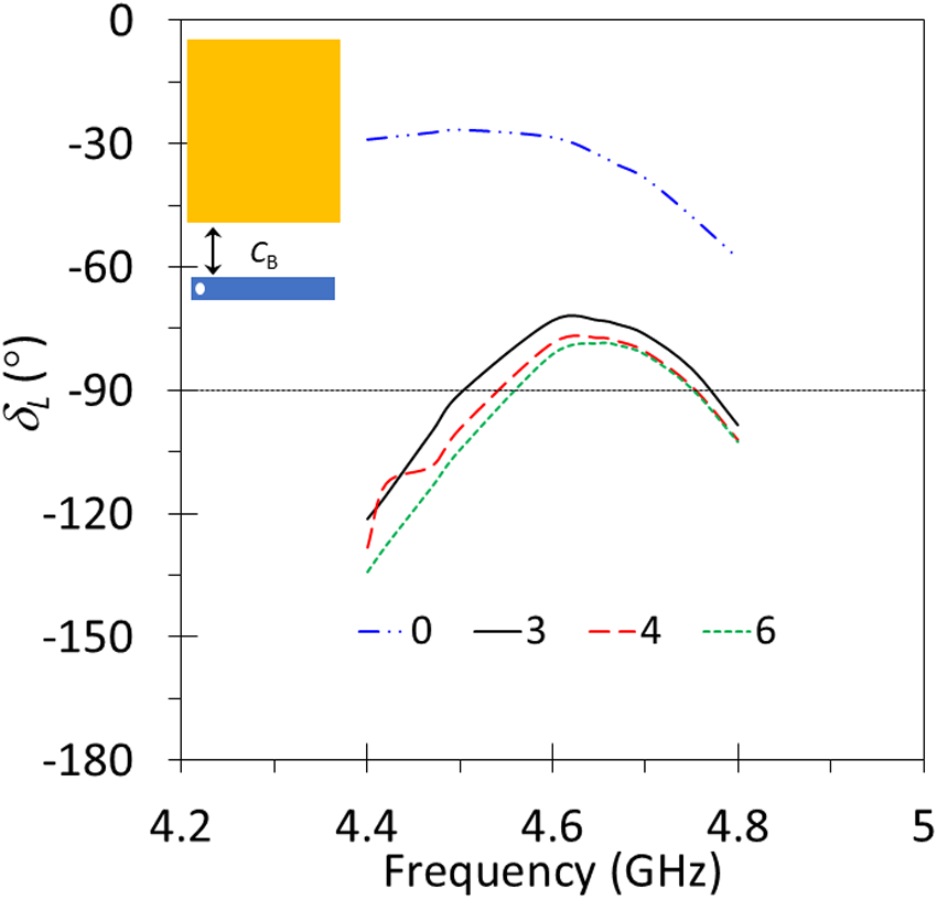
 ${\delta _{\text{L}}}$ can be seen in Fig. 6, where with CB of 0 mm or no distance between the radiator and resonator the
 ${\delta _{\text{L}}}$ is close to 0°. Whereas increasing CB shifts the
 ${\delta _{\text{L}}}$ close to −90° and extending the CB from 3 to 6 mm shows only a slight shift in
 ${\delta _{\text{L}}}$. The CB-tuned 90° phase shift simplifies CP generation without external circuits, advantageous for scalable array designs.
The  ${\delta _{\text{L}}}$ response under variation of CB (unit in mm).

Figure 6 Long description
Delta L A line graph with four curves and a small inset at the upper left. The x-axis label is Frequency (GHz). The x-axis ranges from 4.2 to 5, with labeled ticks at 4.2, 4.4, 4.6, 4.8 and 5. The y-axis label is delta L (degree). The y-axis ranges from 0 at the top down to minus 180 at the bottom, with labeled ticks at 0, minus 30, minus 60, minus 90, minus 120, minus 150 and minus 180. A legend near the bottom center shows four series labeled 0, minus 3, minus 4 and minus 6. Series labeled 0 is a blue dash-dot curve. It starts near delta L about minus 20 at frequency about 4.4, stays near minus 20 to minus 30 through about 4.7, then drops to about minus 60 by about 4.8. Series labeled minus 3 is a black solid curve. It rises from about minus 120 at about 4.4 to a peak near about minus 80 around about 4.65, then falls to about minus 100 by about 4.8. Series labeled minus 4 is a red dashed curve. It rises from about minus 115 at about 4.4 to a peak near about minus 75 around about 4.65, then falls to about minus 95 by about 4.8. Series labeled minus 6 is a green dashed curve. It rises from about minus 130 at about 4.4 to a peak near about minus 85 around about 4.65, then falls to about minus 105 by about 4.8. The inset at the upper left contains a rectangular block and a short horizontal bar with a small label that includes the letter g.
Results and discussion
Parametric study
The optimized results obtained from the iterative process, along with the corresponding responses of S 11 and axial ratio under varying CB, are shown in Fig. 7(a). It is observed that CB exerts a notable impact on both impedance and AR values in the middle and lower band. Specifically, deviations from the 4 mm leads to a reduction in AR bandwidth, indicating a sensitivity to CB alterations. Moreover, variations in S11 degrade with decreases or increases in C B from the 4 mm.
S 11 and axial ratio response in different (a) CB and (b) Gap 1 (all units in mm).

Figure 7 Long description
The image A showing a dual y-axis line graph labeled (a). The horizontal axis is labeled Frequency (GHz), with tick labels at 4, 4.2, 4.4, 4.6, 4.8, 5 and 5.2. The left vertical axis is labeled S subscript 11 (dB), ranging from 0 at the top down to minus 50 at the bottom, with tick labels at 0, minus 5, minus 10, minus 15, minus 20, minus 25, minus 30, minus 35, minus 40, minus 45 and minus 50. The right vertical axis is labeled Axial Ratio (dB), ranging from 0 to 18 with tick labels at 0, 3, 6, 9, 12, 15 and 18. A legend at the top lists six series: S subscript 11, C subscript B equals 2; Axial Ratio, C subscript B equals 2; S subscript 11, C subscript B equals 3; Axial Ratio, C subscript B equals 3; S subscript 11, C subscript B equals 4; Axial Ratio, C subscript B equals 4. The S subscript 11 curves form a deep trough centered around about 4.6 to 4.7 GHz, reaching near the bottom of the scale close to minus 50 dB and rise toward 0 dB near about 4.0 GHz and about 5.2 GHz. The axial ratio curves use the right axis and show higher values near the left and right ends of the frequency range and lower values around the mid band; one axial ratio curve is drawn as a red dashed line, one as a black solid line and one as a blue dashed line. The image B showing a dual y-axis line graph labeled (b). The horizontal axis is labeled Frequency (GHz), with tick labels at 4, 4.2, 4.4, 4.6, 4.8, 5 and 5.2. The left vertical axis is labeled S subscript 11 (dB), ranging from 0 down to minus 50 with tick labels at 0, minus 5, minus 10, minus 15, minus 20, minus 25, minus 30, minus 35, minus 40, minus 45 and minus 50. The right vertical axis is labeled Axial Ratio (dB), ranging from 0 to 18 with tick labels at 0, 3, 6, 9, 12, 15 and 18. A legend at the top lists six series: S subscript 11, Gap subscript 1 equals 3; Axial Ratio, Gap subscript 1 equals 3; S subscript 11, Gap subscript 1 equals 4; Axial Ratio, Gap subscript 1 equals 4; S subscript 11, Gap subscript 1 equals 5; Axial Ratio, Gap subscript 1 equals 5. The S subscript 11 curves again form a deep trough around about 4.6 to 4.7 GHz, approaching the lower end of the scale near minus 50 dB and rise toward 0 dB near about 4.0 GHz and about 5.2 GHz. The axial ratio curves use the right axis and show higher values near the ends of the frequency range and lower values around the mid band; one axial ratio curve is drawn as a red dashed line, one as a black solid line and one as a blue dashed line.
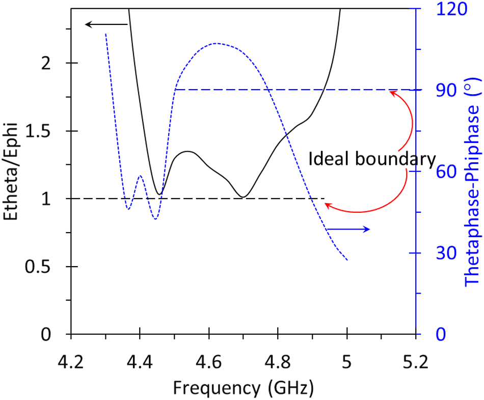
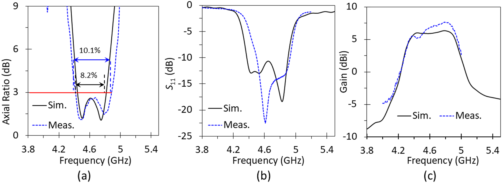
The variation of Gap 1 to the S 11 and AR is depicted in Fig. 7(b). The −10 dB IBw and S 11 are significantly affected by the variation of Gap 1. A wider Gap 1 improves S 11 but degrades the bandwidth, and vice versa. AR is also considered in this optimization within the same parametric study, Gap 1 influences the AR in the middle and lower bands. Two minimum optimized ARs occur at 4.49 and 4.76 GHz, resulting in 380 MHz ARBw or 8.2%. The characteristic of the RHCP can be presented by the magnitude ratio of the orthogonal electrical field and its phase difference, as shown in Fig. 8. The ratio of E θ and E Φ magnitude over the bandwidth 4.5–4.8 GHz is varied between the range 1.04 to 1.4 while the phase differences are between 43° and 106°. These values are close to the ideal value of 1° and 90°.
Magnitudes and phases of the E θ and E Φ.

Figure 8 Long description
The graph shows two plotted lines versus frequency. The x-axis is labeled Frequency (GHz), ranging from 4.2 to 5.2 with tick marks at 4.2, 4.4, 4.6, 4.8, 5.0 and 5.2. The left y-axis is labeled Etheta over Ephi, with tick marks at 0.5, 1.0, 1.5, 2.0 and 2.5. A black line starts near 2.5 at about 4.3, drops to about 1.0 near 4.4, rises to about 1.3 near 4.5, dips to about 1.0 near 4.6, then rises steadily to about 2.0 by about 5.0 and remains near 2.0 to about 5.2. The right y-axis is labeled Phase difference (degree), ranging from 0 to 120 with tick marks at 0, 30, 60, 90 and 120. A blue dashed line starts near 110 at about 4.3, drops to about 40 near 4.4, rises to about 60 near 4.45, drops again to about 40 near 4.5, then rises to a peak near 110 around 4.7 to 4.75 and then declines to about 30 by about 5.0. A horizontal dashed line is drawn at 90 on the phase difference scale. The text Ideal boundary is placed near the right side of the plot, next to a short red curved segment.
Measurement
To enhance the confirmation of both the proposed method and the simulation outcomes, we construct and assess a prototype of the CP patch antenna. The antenna is fabricated on two layers of Roger Duroid 5880, each with a thickness of 1.575 mm and a permittivity of 2.2, as shown in Fig. 9 (a)–(c). In this study, the fabricated antenna is measured using the Rohde Schwarz ZNB-40 vector network analyzer as shown in Fig. 9(d). The measured ARBw is depicted in Fig. 10(a), where the two minimum axial ratios are observed at 4.48 and 4.79 GHz. The presence of two distinct minimum ARs implies that the antenna achieves approximately three times the AR bandwidth of the second-order filter-based design in Ref. [Reference Cahyasiwi, Zulkifli and Rahardjo28]. The AR bandwidth measurement is 10.1% span from 4.41 to 4.88 GHz or 1.9% wider than the simulation result. The reflection coefficients obtained through simulation and measurement are plotted in Fig. 10(b). The reflection coefficient result shows that the measured antenna covers a wide −10 dB IBw from 4.49 to 4.93 GHz, equivalent to a 9.04% fractional bandwidth, which is 2.16% narrower than the simulation result of 11.2%. The lower frequency shifts by 120 MHz from 4.37 to 4.49 GHz, while the upper frequency exhibits a slight shift of 20 MHz. The discrepancies observed in the ARBw and IBw results are attributed to fabrication imperfections, angular averaging, and off-boresight improvements during the AR measurement. The simulated gain response remains flat within a frequency band centered at 4.65 GHz and gradually decreases on both sides of this band, demonstrating desirable filtering characteristics that are better than the previous design in Ref. [Reference Cahyasiwi, Zulkifli and Rahardjo28]. The measurement result exhibits a slightly lower gain at lower frequencies compared to the simulation result, as shown in Fig. 10(c). This discrepancy is attributed to a higher measured reflection coefficient (S 11) in this region, indicating suboptimal signal transmission. Conversely, at higher frequencies, the measured gain is rather higher than the simulated result. This is likely caused by an air gap between the stacked substrates above the second resonator, which may have formed during measurement and contributed to the gain increase. The maximum gain of simulation and measurement is 6.30 at 4.65 GHz and 7.60 dBic at 4.81 GHz, respectively.
The fabricated antenna (a) radiator, (b) feedline, (c) assembled prototype, and (d) measurement.

Figure 9 Long description
The image A shows a square copper patch on a blue substrate, representing the radiator of the CP patch antenna. The image B displays the feedline with copper strips on a similar substrate. The image C shows the assembled prototype with a connector attached at the bottom. The image D depicts the measurement setup with the antenna placed in an anechoic chamber, surrounded by absorptive material.
Simulated and measured results of (a) axial ratio, (b) S 11, and (c) gain of the proposed design.

Figure 10 Long description
The image A showing a line graph with the y-axis label “Axial Ratio (dB)” and x-axis label “Frequency (GHz)”. The x-axis ranges from 3.8 to 5.4. The y-axis ranges from 0 to 9. A legend shows “Sim.” and “Meas.” Two curves are plotted. The curves stay close to 9 at about 3.8, then drop to values close to 0 around the mid 4 range, then rise again toward 9 by about 5.0. A bracket annotation reads “10.1 percent”. A second bracket annotation reads “8.2 percent”. The image B showing a line graph with the y-axis label “S subscript one one (dB)” and x-axis label “Frequency (GHz)”. The x-axis ranges from 3.8 to 5.4. The y-axis ranges from negative 25 to 0. A legend shows “Sim.” and “Meas.” Two curves are plotted. Both curves start close to 0 at about 3.8, decrease to a minimum below negative 20 around the mid 4 range, then increase back toward 0 by about 5.0. The image C showing a line graph with the y-axis label “Gain (dBi)” and x-axis label “Frequency (GHz)”. The x-axis ranges from 3.8 to 5.4. The y-axis ranges from negative 10 to 10. A legend shows “Sim.” and “Meas.” Two curves are plotted. Both curves rise from values below 0 around 3.8 to values around 6 to 8 through the mid 4 range, then decrease toward 0 by about 5.0.
The far-field patterns were measured at two frequency points (4.48 and 4.79 GHz), corresponding to two minima in the AR response. The normalized gain patterns for RHCP and left-hand circular polarization for both frequencies are depicted in Figs. 11 and 12. The cross-polarization gain is roughly 20 dB less than the co-polarization gain in the direction of the main beam. The radiation patterns reveal a coherent beam shape in co-polarization, underlining the stable performance of the radiation. The 3 dB beamwidths measured in the phi = 0° at two different frequencies are 76.5° and 78.6°, respectively. Similarly, in the phi = 90°, the measured 3 dB beamwidths are 84° and 77.5° at the corresponding frequencies.
Normalized radiation pattern at 4.49 (simulation)/4.48 (measurement) GHz.

Figure 11 Long description
Normalized radiation pattern at 4.49 (simulation)/4.48 (measurement) GHz. Two polar plots illustrate normalized gain patterns for right-hand circular polarization and left-hand circular polarization at phi equals 0 degrees and phi equals 90 degrees. The radial axis represents gain in decibels, with values ranging from minus 10 to minus 40. The first plot at phi equals 0 degrees shows four curves: measured right-hand circular polarization at 4.48 gigahertz (black dotted), simulated right-hand circular polarization at 4.49 gigahertz (black solid), measured left-hand circular polarization at 4.48 gigahertz (red dotted) and simulated left-hand circular polarization at 4.49 gigahertz (red solid). The main lobe direction is around 0 degrees, with peak levels near minus 10 decibels. The second plot at phi equals 90 degrees displays similar curves, with main lobes around 90 degrees and peak levels also near minus 10 decibels. The simulated curves generally show smoother lobes compared to measured curves, indicating stable performance. Notable discrepancies occur at specific angles, with cross-polarization gain roughly 20 decibels less than co-polarization gain in the main beam direction.
Normalized radiation pattern at 4.76 (simulation)/4.79 (measurement) GHz.

Figure 12 Long description
The plots are labeled “Phi equals 0 degree” and “Phi equals 90 degree.” Each plot is a polar graph with angle markings around the circle at 0, 30, 60, 90, 120, 150, 180, 210, 240, 270, 300 and 330. Concentric radial rings are labeled 0, minus 10, minus 20, minus 30 and minus 40. In each polar graph, four line styles are shown in a legend: “Measured RHCP 4.79 GHz,” “Simulated RHCP 4.76 GHz,” “Measured LHCP 4.79 GHz,” and “Simulated LHCP 4.76 GHz.” The RHCP curves are drawn as a solid line for measured and a dashed line for simulated. The LHCP curves are drawn as a dotted line for measured and a dash dot line for simulated. In the “Phi equals 0 degree” plot, the RHCP curves form a larger lobe on the right side of the plot near angles around 60 to 120, with the curve closer to the 0 ring than the other curves in that region. The RHCP curves dip inward toward the minus 30 to minus 40 rings near angles around 180 to 210. The LHCP curves stay closer to the minus 20 to minus 40 rings over most angles, with a deeper inward dip near angles around 180. In the “Phi equals 90 degree” plot, the RHCP curves form a broad lobe on the right side near angles around 60 to 120 and another outward bulge on the left side near angles around 240 to 300. The RHCP curves dip inward near angles around 180. The LHCP curves remain more inward than the RHCP curves across most angles, with inward regions near angles around 180 and around 0.
Table 1 shows the comparison of the proposed design with the previous studies in terms of the method and the ARBw results. It is known that orthogonal feedlines can achieve a wider ARBw than the single feedline filtering antenna. The two orthogonal feedlines were implemented in Ref. [Reference Wu, Zhang and Zhu10, Reference Wu, Zhang and Zhu20] using two substrate layers, while our proposed design, utilizing a single feedline, achieves a wider ARBw compared to those two designs. The circular radiator with C-shaped perturbation in Ref. [Reference Rai, Sigroha, Tyagi, Das and Sharma15] achieves a wide ARBw; however, the CP generation and filtering functions were designed separately, and the perturbation results in a lower gain than our design. Reference [Reference Qin, Han, Zhang, Mao and Zhu21] employs an omnidirectional antenna, which should theoretically have a wider bandwidth. However, despite emphasizing its dual-band performance, the ARBw, IBw, and gain results fall below those of our design. In Ref. [Reference Cheng, Huang, Huang and Yang23], using coaxial probe and foam between the two substrates layer make the design complicated, especially if we need to design an array antenna, though it has wider IBw, the ARBw is narrower than our design. The widest impedance and ARBws in this comparison are reported in Refs. [Reference Zhou, Pan, Cheng, Yang, Li and Huang25] and [Reference Wang, Zhang, Ye and Liu27], the design using multiple layers and air gap layers to achieve a wider ARBw, however the IBw is wider than ARBw, while in our design, the ARBw is wider than the IBw. Additionally, the use of multiple substrate layers with air gaps in between results in a high-profile and complex structure. The proposed single-feed design achieves a competitive ARBW while maintaining significantly reduced structural complexity compared to multi-layer CP filtering antennas. Our proposed design demonstrates an ARBw that is nearly 300% wider and an IBw that is almost 200% wider than the previous study in Ref. [Reference Cahyasiwi, Zulkifli and Rahardjo28], which also uses a single λ/4 resonator. However, the report lacked both a phase shifter and higher-order filter analysis. The improvement in the proposed design is achieved by incorporating an additional resonator.
Comparison of the proposed design with previous published CP filtering antenna

Table 1 Long description
The table compares multiple published CP filtering antennas by normalized size (L×W×T in λ0), whether CP and filtering are integrated, CP generation method, whether phase-shifter analysis is included, impedance and axial-ratio bandwidths (IBw/ARBw), substrate layering, and gain (dBic). Only two entries integrate CP and filtering: Ref. [28] and this work. This work is 0.775×0.775×0.048 λ0, uses third-order orthogonal resonators, includes phase-shifter analysis, achieves 9.04% IBw and 10.1% ARBw, uses 2 substrate layers, and has 7.6 dBic gain. Ref. [28] is smaller (0.69×0.69×0.048 λ0) but has narrower bandwidths (4.7%/3.2%) and lower gain (6.2 dBic), and does not report phase-shifter analysis. Several non-integrated designs report very wide bandwidths (e.g., [25] 59.0%/51.8% and [27] 58.3%/46.9%) but use thicker structures with multiple air-gap layers (T up to 0.29–0.34 λ0). Gains range from about 0–1.5 dBic in the smallest radiator-perturbation design [21] to 8.54 dBic in [25], with many mid-size designs around 5–7.6 dBic. One entry ([21]) lists two IBw/ARBw pairs, indicating multiple operating bands or cases, so direct one-to-one comparison may depend on the reported band definitions.
Conclusion
In this study, a wide ARBw filtering antenna using orthogonal resonators has been designed and measured. The orthogonal resonators are modelled with a rectangular radiator and two quarter-wavelength resonators integrated through a third-order filter design. The CP filtering antenna is determined by three key factors: the ratio of length to width of the rectangular radiator, the gap between the radiator and the resonator, and the gap between the two resonators. The realized model results in an 10.1% ARBw and 9.04% IBw, complemented by a gain exhibiting filtering characteristics. The proposed design verifies that using the orthogonal resonators method with a higher order filter for integrating a filter and an antenna can effectively achieve a wider ARBw CP filtering antenna using only a single feed line. Future work will primarily focus on the application of the proposed CP filtering antenna in energy harvesting systems.
Acknowledgements
The authors thank the Electrical Department, Faculty of Engineering, Universitas Indonesia, for providing the measurement laboratory and CST software; Indonesia Digital Test House for providing the measurement laboratory; and Eka Setya Nugraha from University Telkom Purwokerto, for assisting with the measurement.
Competing interests
The authors declare none.

Dwi Astuti Cahyasiwi received her Bachelor's, Magister, and Doctoral degrees in Electrical Engineering from the Universitas Indonesia in 1997, 2009, and 2022. She received an Excellent Scholarship for Indonesia’s Lecture (Beasiswa Unggulan Dosen Indonesia/BUDI-LPDP) for her Doctoral degree. She has been a member of the IEEE Antenna and Propagation Society (AP-S) since 2021 and a reviewer of IEEE Access since 2020. She was a recipient of the Best Student Paper Award at the 2019 IEEE Conference on Antenna Measurement and Applications (CAMA). She has been a lecture in Electrical Engineering Department Universitas Muhammadiyah Prof Dr. HAMKA since 2000. Her research interests are integration design of antenna and filter, multiple-input multiple-output (MIMO), dual-polarized antenna systems, metasurface, polarization converter, and microwave circuits.

Fitri Yuli Zulkifli received her degree in electrical engineering for Bachelor (1997) and Ph.D. (2009) from Universitas Indonesia (UI), while her M.Sc. degree from Karlsruhe Institute of Technology, Germany (2002). Her research interests are antenna, propagation, microwave, and the field of telecommunication. She joined the Antenna Propagation and Microwave Research Group (AMRG) at UI in 1997 and has been a lecturer in the electrical engineering department at UI since 1998. She has published more than 200 papers in journals/conference proceedings and received more than 40 research grants. She now leads “Laboratory Prof. Fitri Yuli Zulkifli” and also the head of professional engineering study program in UI. From 2011 to 2012, she became the joint chapter chair of MTT/AP Indonesia. In 2017–2018, she was the IEEE Indonesia Section Chair and in 2019–2022, she serves as committee member for R10 Conference and Technical Seminar and Conference Quality Management.

Ashif Aminulloh Fathnan received a Doctoral degree from the University of New South Wales (UNSW), Canberra, Australia, in February 2021. He is now a Senior Researcher at the Research Center for Telecommunication, National Research and Innovation Agency (BRIN), Indonesia, and a Lecturer at the Department of Electrical Engineering, Telkom University, Indonesia. From 2021 to 2024, he was a distinctive researcher with the electromagnetics group at Nagoya Institute of Technology, Japan. He received a postdoctoral fellowship award from the Japan Society for the Promotion of Science (JSPS) in 2022, LPDP Doctoral Scholarship (2017–2021) from the Ministry of Finance, Republic of Indonesia, Young Scientist Award from the International Union of Radio Science (URSI) and Dean’s Award for Outstanding PhD Theses from UNSW Australia in 2021. His current research interests include: spectral and spatial dispersion of metasurfaces; tunable metasurfaces for sensing, imaging and communication; and nonlinear metasurfaces.

Aditya Inzani Wahdiyat received the bachelor’s degree in electrical engineering from Universitas Indonesia (UI) in 2010. He was an application engineer at CST Malaysia from 2010 to 2015. From 2015 to 2021, he was an electronic engineer with The Agency for the Assessment and Application of Technology, Indonesia. He has been working as a researcher at National Research and Innovation Agency, Indonesia. His research interests include electromagnetic applications, wave propagation, and the analysis and design of metamaterial and microwave engineering.

Yus Natali received her B.Eng. (S.T.) degree in telecommunication engineering from Sekolah Tinggi Teknologi Telkom, Bandung, in 2001, and the M.Eng. (M.T.) degree in telecommunication engineering from the Department of Electrical Engineering, Universitas Indonesia, Depok, in 2009, where she graduated with a Doctoral degree in electrical engineering (Dr.) in 2023. She has been a Lecturer at Akademi Telkom Sandhy Putra Jakarta, since 2003, and the Telkom University in Jakarta, Indonesia, since 2023. She has been the Head of theTelecommunications Engineering Study Program, Akademi Telkom Sandhyputra Jakarta, and Telkom University. Her research interests include radio over fiber, distributed antenna systems, microwave photonics, wireless communication, electro-optic modulator, integrated antenna-EO modulator, and optical networks. She is also one of the Editor of JICT Telkom University.

Teguh Firmansyah was born in Subang, Indonesia. He received the B.Eng. and M.Eng. degree in electrical engineering from the Department of Electrical Engineering, Universitas Indonesia, in 2010 and 2012, respectively, and the Dr.Eng. degree from Shizuoka University, Japan, in 2022. In 2012, he joined the Department of Electrical Engineering, Universitas Sultan Ageng Tirtayasa, as a Researcher and a Lecturer. He holds two patents for wideband antenna and multiband antenna. His research interests include microwave circuits for various applications and developing multifunctional sensors using acoustic, plasmonic, and microwave resonators.

Dian Widi Astuti was born in Jakarta, Indonesia. She received the B.Eng. and M.Eng. from Universitas Mercu Buana, Jakarta, Indonesia, and her Ph.D. degree from Universitas Indonesia in 2022. Since 2012, she has been a lecturer and joint member of the electromagnetic and telecommunication Laboratory at Universitas Mercu Buana, Jakarta. Her current research interests include microwave and millimeter-wave passive component design. She has been involved in the 2019 IEEE International Conference on Antenna Measurement Applications (CAMA), Bali, in October 2019, and the 2024 IEEE Asia Pacific Microwave Conference (APMC), Bali, in November 2024, as Secretary.

Eko Tjipto Rahardjo received B.Eng degree from Universitas Indonesia, Indonesia, in 1981, an M.S. degree from the University of Hawaii, USA, in 1987, and a Ph.D. degree from Saitama University, Japan, in 1996, all in electrical engineering. He has been the Director of Antenna Propagation and Microwave Research Group (AMRG), Universitas Indonesia. His research interests include antenna engineering, wave propagation, microwave circuits and communication systems, and telecommunication system regulations. He has been published and presented more than 200 research articles both national and international journals and symposiums. He is a member of the IEEE Antenna and Propagation Society (AP-S) and the IEEE Microwave Theory and Technique Society (MTTS) and has been actively participated in National and International Committee as International Advisory Board, Steering Committee or General Chair in International Symposium on Antenna and Propagation (ISAP), Asia Pacific Microwaves Conference (APMC) and IEEE Conference on Antenna Measurement and Applications (CAMA).