Introduction
The topic of motion adaptation in the fly visual system has been a subject of much research and debate in recent decades (Strausfeld & Campos-Ortega, Reference Strausfeld and Campos-Ortega1977; Maddess & Laughlin, Reference Maddess and Laughlin1985; Egelhaaf & Borst, Reference Egelhaaf and Borst1989; Harris et al., Reference Harris, O’Carroll and Laughlin1999, Reference Harris, O’Carroll and Laughlin2000; Reisenman et al., Reference Reisenman, Haag and Borst2003; Kurtz, Reference Kurtz2007). Flies are a particularly attractive system in which to study motion adaptation both because the features of adaptation observed in their large movement-detecting lobula plate tangential cells (LPTCs) are very similar to those observed in primate visual systems (Kohn & Movshon, Reference Kohn and Movshon2003) and because the size and accessibility of these cells makes them amenable to electrophysiological recordings. LPTCs are wide field sensitive and directionally selective (Hausen, Reference Hausen and Ali1984) and are thought to integrate the output of an array of small-field sensitive elementary motion detectors (EMDs; Egelhaaf et al., Reference Egelhaaf, Borst and Reichardt1989). Many details of motion adaptation in LPTCs have been reported in the literature; we provide a brief summary of the most relevant results below.
Motion adaptation results in LPTC responses that are strongest at the onset of a motion stimulus and decay during continuous motion stimulation until an asymptotic steady-state response level is approached. The rate of decay of the response was shown by Maddess and Laughlin (Reference Maddess and Laughlin1985) to be strongly dependent on the temporal frequency of the stimulus and less sensitive to the contrast or to the spatial frequency of the grating. Importantly, these authors concluded that this type of adaptation does not originate in the tangential cell itself but rather appears to be localized in the EMDs.
Adaptation has also been studied by focusing on the effect that a high-contrast high-frequency moving grating (referred to as a “strongly adapting stimulus”) has on a subsequent test stimulus. Harris et al. (Reference Harris, O’Carroll and Laughlin2000) applied a test stimulus before and after motion adaptation with a strongly adapting stimulus of a fixed high contrast and fixed temporal and spatial frequency. By computing the mean membrane potential of LPTCs during the presentation of a test stimulus with fixed temporal and spatial frequency but of different contrast levels, they produced contrast response curves before and after motion adaptation. The contrast response curve exhibited a sigmoid-like shape, saturating for high-contrast stimuli. Such contrast saturation has been previously observed and modeled (Egelhaaf & Borst, Reference Egelhaaf and Borst1989; Rivera-Alvidrez & Higgins, Reference Rivera-Alvidrez and Higgins2005).
Three components of the adaptation induced by a strongly adapting stimulus moving in the cell’s preferred direction were identified by Harris et al. (Reference Harris, O’Carroll and Laughlin2000). First, a general reduction in the cell’s baseline voltage level was observed immediately after the strongly adapting stimulus. This resulted in smaller mean responses to the postadaptation test stimulus and thus, in a downward shift in the contrast response curve. This adaptation component was referred to as an afterpotential or as the “waterfall effect” because of its similarity to the waterfall illusion in humans (Wohlgemuth, Reference Wohlgemuth1911). The afterpotential was hyperpolarizing if the cell was excited during the adapting period and depolarizing if the cell was inhibited. The afterpotential thus appears to be activity dependent and directionally selective. The second component of adaptation identified was a lower contrast saturation level. This reduction in output range persisted even when the afterpotential was subtracted. Third, even after accounting for both of the previously mentioned components, a postadaptation test stimulus of any given contrast produced a smaller LPTC response compared to the response to the preadaptation test stimulus of the same contrast. This was reflected in a rightward shift of the postadaptation contrast response curve with respect to the preadaptation curve and was referred to as a reduction in contrast gain. All three components appear to be generated through separate mechanisms, with the contrast gain reduction contributing the most to motion adaptation. While contrast gain reduction appears to be localized in the EMDs, the afterpotential and the output range reduction were suggested to originate in the tangential cell itself. Recent work by Kurtz (Reference Kurtz2007) has shed some light on the neuronal mechanisms of adaptation for the two components attributed to the tangential cell but not for contrast gain reduction. For the rest of the paper, we will focus our attention on the contrast gain reduction component of adaptation. We do not model the other two components of adaptation since they most likely occur at the tangential cell level.
Both Maddess and Laughlin (1985) and Harris et al. (Reference Harris, O’Carroll and Laughlin2000) reported that contrast gain reduction is more pronounced after adaptation with motion than with flicker. Moreover, Harris et al. (Reference Harris, O’Carroll and Laughlin2000) also reported that contrast gain adaptation does not depend on the direction of motion. Both adaptation with a stimulus moving in the preferred direction and adaptation with a stimulus moving in the antipreferred direction result in similar reductions in contrast gain. Furthermore, the same contrast gain reduction is produced by a stimulus moving along the vertical axis, even though the LPTCs they recorded from (HS cells) do not respond to vertical motion.
When operating in the high-contrast range, LPTC responses become saturated, and variations in the stimulus contrast level result in little or no change in the response of the cell. Saturation reduces the cell’s sensitivity to the stimulus contrast. A similar region of low sensitivity has been reported in the temporal frequency tuning of the cell at frequencies, which elicit high response levels, and was also attributed to saturation (Harris et al., Reference Harris, O’Carroll and Laughlin1999). Harris et al. (Reference Harris, O’Carroll and Laughlin2000) proposed that the function of contrast gain reduction could be to “release” the motion pathway from saturation, allowing it to restore high sensitivity to fluctuations in the stimulus parameters. Harris et al. (Reference Harris, O’Carroll and Laughlin2000) hypothesized that in order for contrast gain reduction to protect the system from saturation, it should occur before the EMD circuitry where this saturation arises.
Based upon the conclusions about motion adaptation summarized above and building upon a previously published neuronally based model of elementary motion detection (Higgins et al., Reference Higgins, Douglass and Strausfeld2004; Melano & Higgins, Reference Melano and Higgins2005; Rivera-Alvidrez & Higgins, Reference Rivera-Alvidrez and Higgins2005), in this paper, we present a neuronally based model of the contrast gain reduction component of motion adaptation. The components of this model correspond directly to specific identified neurons in the fly brain, and the model implicates synaptic depression in a graded potential synapse as the neuronal basis of contrast gain reduction.
The neuronally based EMD model
The Hassenstein–Reichardt (HR) correlation model of motion detection (Hassenstein & Reichardt, Reference Hassenstein and Reichardt1956) is perhaps the most long-lived computational model in visual neuroscience and is commonly used to predict the responses of fly EMDs. However, because it does not (and was never intended to) provide any insight into the neuronal implementation of this computation, efforts have been made to compile a large volume of anatomical, electrophysiological, and histological evidence into a neuronally based EMD model (Higgins et al., Reference Higgins, Douglass and Strausfeld2004). Unlike the HR model, a neuronally based model may serve as a substrate for the understanding of the neural basis of motion detection and can be used to derive biologically testable hypotheses about the network of cells and synapses that it represents. The neuronally based EMD model has been shown to be as successful as the HR model in predicting the responses of tangential cells to a wide variety of complex visual stimuli.
The neuronal circuit, diagrammed in Fig. 1, includes lamina amacrine cells, lamina monopolar cells, the basket T-cell T1, the transmedullary cells Tm1 and Tm9, the T5 bushy T cell, and an inhibitory interneuron. The foundations of the model are detailed elsewhere (Higgins et al., Reference Higgins, Douglass and Strausfeld2004). Briefly, amacrine cells receive photoreceptor input and have been shown to synapse onto the T1 basket T cell (Campos-Ortega & Strausfeld, Reference Campos-Ortega and Strausfeld1973). Because T1 shows an inverted response to that of the photoreceptors and has a small sustained component (Douglass & Strausfeld, Reference Douglass and Strausfeld2004), the signal from the amacrine cell in the model is sign inverted and filtered with a “relaxed” high-pass filter (see Higgins et al., Reference Higgins, Douglass and Strausfeld2004 for details) containing a small low-pass component (to allow for a small sustained signal to be transmitted to T1). The lamina monopolar cell L2, also receiving photoreceptor input, is modeled with a sign-inverted high-pass filter, as no sustained component has been detected in the L2 cell response (Coombe et al., Reference Coombe, Srinivasan and Guy1989). Both L2 and T1 are presynaptic to Tm1 (Campos-Ortega & Strausfeld, Reference Campos-Ortega and Strausfeld1973), but while L2 receives input from the photoreceptor in the same optic cartridge, T1 carries signals from amacrine cell processes expanding to neighboring units. One-dimensional and two-dimensional versions of the model have been proposed, differing only in the way that T1 is computed. In the one-dimensional model, T1 is computed by adding low-pass filtered amacrine signals from two neighboring photoreceptors, as shown in Fig. 1. In the two-dimensional model, low-pass filtered amacrine signals from a hexagonal array of neighboring photoreceptors are added at T1. The response of the transmedullary cell Tm1 is computed by adding T1 and the local signal from L2. Tm1 responds to motion in any orientation, and because it receives both a local input and the delayed (low-pass filtered) signals from neighboring visual units, it is a candidate for encoding nondirectional motion (Dyhr & Higgins, Reference Dyhr and Higgins2010) in its amplitude. This implies that the cell is sensitive to motion, but unlike a directionally selective cell, it is unable to distinguish between motion in different directions.
The one-dimensional neuronally based model of elementary motion detection. (a) The model incorporates amacrine cells (Am), lamina monopolar cells (L2), basket T cells (T1), two types of transmedullary cells (Tm1 and Tm9), T5 bushy T cells (T5-R and T5-L), and an inhibitory interneuron (IIN). Circles represent computational processing stages, and neuron labels next to arrows show where the emulation of a particular cell can be found in the model. Arrows represent excitation, lines with filled circles represent inhibition, and lines with open circles represent shunting inhibition. Relaxed high-pass filter (RHPF) represents a high-pass filter (HPF) with a small low-pass component. A filter preceded by a negative sign indicates that the output of the filter was sign inverted. The inputs from T5 are rectified (POS) and subtracted by the tangential cell model. The center-surround spatial filter was implemented at the level of amacrine and L2 cells to attenuate the mean luminance in the input image. The G.C. block models pattern size saturation, also called gain control (ge and gi refer to excitatory and inhibitory conductances). The contrast saturation is inherent in the biophysical shunting inhibition at the level of T5 cells. The “A” blocks model adaptation as described in the text. (b) The center-surround spatial filter computes the difference between two Gaussian filters of different widths. The value of the weight parameter can be adjusted between 0 and 1 to control the amount of spatial mean luminance in the motion pathway. When the weight is equal to 1, the subtraction between the two Gaussian filters eliminates all the spatial mean luminance in the input signals. Smaller values of the weight allow the preservation of more spatial mean luminance in the inputs.

While histological studies suggest a role for Tm1 as an excitatory input to the T5 cell, a second transmedullary cell, Tm9, is likely an inhibitory synaptic input (Sinakevitch & Strausfeld, Reference Sinakevitch and Strausfeld2004). In addition, the processes of Tm1 coincide with Tm9. Both Tm1 and Tm9 terminate at the level of T5, but the Tm9 unit is displaced one visual sampling unit. The interaction of these three cells is modeled as a Barlow–Levick motion detector (Barlow & Levick, Reference Barlow and Levick1965), which computes motion through the interaction of an excitatory input (Tm1) with a delayed inhibitory input from a neighboring unit (Tm9). The inhibition from Tm9 is shunting, producing the nonlinearity required for directional selectivity. Opponent directional selectivity at the level of T5 is achieved through an inhibitory interneuron, revealed by immunohistochemical studies (Sinakevitch & Strausfeld, Reference Sinakevitch and Strausfeld2004). In order to reproduce data from Single et al. (Reference Single, Haag and Borst1997), the T5 inputs to the tangential cell are rectified and subtracted (see Melano & Higgins, Reference Melano and Higgins2005 for details). This form of integration has recently been shown to support fast-scale adaptive changes observed in fly tangential cells (Neri, Reference Neri2007), previously thought to another component of motion adaptation. The model also supports saturation with pattern size (also called “gain control”) implemented in the blocks labeled G.C., as described in Borst et al. (Reference Borst, Egelhaaf and Haag1995) and Single et al. (1997) and detailed in the Materials and Methods section.
In this paper, we make three primary changes to the model from the version of Higgins et al. (Reference Higgins, Douglass and Strausfeld2004). First, a center-surround spatial filter has been added to the first stage of the model, as shown in Fig. 1. This change was necessary to allow the model to distinguish motion from field flicker and is detailed below. The second change is the blocks labeled “A,” modeling adaptation via contrast gain reduction. The final change is that contrast saturation is implemented at the level of T5 cells using a model for synaptic interaction outlined in Koch (Reference Koch1999) to reflect the biophysics of neurons, rather than with saturating elements as in previous versions of the model. This change, described below, was also necessary to support contrast gain adaptation.
Center-surround spatial filtering
The lamina is believed to be the site of redundancy reduction in the insect visual pathway (Laughlin et al., Reference Laughlin, Howard and Blakeslee1987). Studies from Sinakevitch and Strausfeld (Reference Sinakevitch and Strausfeld2004) suggest that both type 1 amacrine cells (AM1) and type 2 amacrine cells (AM2) have widespread networks such that the response of a single optic cartridge can travel and spread across several levels of neighboring optic cartridges. L2 cells from neighboring optic cartridges do not have connections to one another (Strausfeld & Nässel, Reference Strausfeld, Nässel and Autrum1980), but they exhibit the center-surround spatial antagonism (Srinivasan et al., Reference Srinivasan, Laughlin and Dubs1982) found in cells belonging to a spreading network. There is no direct synaptic interaction between amacrine cells and L2 cells; however, both cells are both pre- and postsynaptic to the photoreceptor cells (Strausfeld & Nässel, Reference Strausfeld, Nässel and Autrum1980).
Combining these pieces of information, we hypothesize a series of synaptic interactions between the photoreceptor cells, the amacrine cells, and the L2 cells in the lamina as follows. AM1 and AM2 cells receive synaptic inputs from photoreceptor cells. The signals spread across the network of AM1 cells and the network of AM2 cells, such that each AM1 or AM2 cell represents the weighted sum of its local signals and the signals from its neighboring optic cartridges. An inhibitory interaction between the AM1 and AM2 cells (that could possibly occur at the amacrine cell level or the photoreceptor cell level) results in the subtraction of the AM1 responses from the AM2 responses before the signals reach the L2 cell level. The difference of these two Gaussian filters results in a center-surround receptive field with an excitatory central region and inhibitory sidelobes. These signals are hypothesized to synapse back onto the photoreceptor cells, which then relay the signals to the L2 cells through their synaptic connection. In this way, the photoreceptor cells act as the liaison between the AM cells and the L2 cells. It has been widely accepted that the adaptive and filtering mechanisms observed in photoreceptor cells are not intrinsic to themselves but rather the result of a series of synaptic connections to downstream neurons such as the AM cells and the L2 cells (Juusola et al., Reference Juusola, Weckstrom, Uusitalo, Korenberg and French1995).
Working from this hypothesis, we propose that the center-surround spatial filter at the L2 level is composed of the subtraction of a Gaussian spreading network of AM1 cells from a similar spreading network of AM2 cells. The filtered output from this processing by the amacrine cells is relayed to and shared by the L2 cells. To reflect this center-surround spatial filtering in the two-dimensional EMD model, we add a computational module (Fig. 1) that is mathematically described by eqn. (1):

with


where AMout(i) is the output signal from the amacrine network at the ith time step, f(i) is the two-dimensional array of photoreceptor responses at the ith time step, * denotes the convolution operation, g 1 and g 2 are the Gaussian spatial filters (with n 1 and n 2 representing the two spatial dimensions of the filters), and w is a scalar weight used for determining the amount of attenuation of the spatial mean component of the visual stimulus. Each Gaussian filter is normalized such that the sum of the coefficients is equal to 1, to ensure that signals are passed through with unity gain. The subtraction represents the inhibitory interaction between AM1 and AM2 cells. The use of the spatial Gaussian filters g 1 and g 2 represent the spreading networks of AM1 and AM2 cells, respectively. This center-surround type spatial filter allows the preservation of motion information while eliminating the spatial mean luminance from wide-field flickering stimuli by computing the difference between the two Gaussian filters of different widths, σ 1 and σ 2, with σ 1 larger than σ 2. In addition, the value of w can be adjusted between 0 and 1 to control the amount of spatial mean luminance in the motion pathway since recorded data from the LPTCs did reflect some responses to flickering visual stimuli. A w value of 0 allows undiminished passage of the spatial mean component, while a value of 1 completely removes the spatial mean luminance from the image.
A model of contrast gain adaptation
Contrast gain reduction in fly visual interneurons reduces the cell’s response during sustained motion stimulation. Such a response is similar to the type of responses exhibited in many mammalian cortical neurons, including neurons in the primary visual cortex V1 (Chance et al., Reference Chance, Nelson and Abbott1998). These neurons respond to new high-frequency stimuli in a stronger manner compared to their responses to sustained stimuli over the same frequency range. In rats, short-term synaptic depression (Abbott et al., Reference Abbott, Sen, Varela and Nelson1997; Varela et al., Reference Varela, Sen, Gibson, Forst, Abbott and Nelson1997) has been identified in V1 neurons as being responsible for the reduction in their response to sustained stimuli (Chance et al., Reference Chance, Nelson and Abbott1998).
Given the parallels between the responses of the visual neurons in insects and mammals, it is reasonable to postulate that a phenomenon such as synaptic depression could be occurring somewhere in the fly’s EMD pathway. All the neurons which we have previously mentioned as being in the EMD pathway appear to be nonspiking (graded potential) neurons, and chemical synapses appear to be responsible for signal transmission between these neurons both by anatomical observation and due to the presence of neurotransmitters (Sinakevitch & Strausfeld, Reference Sinakevitch and Strausfeld2004). These synapses signal both increases and decreases from the resting potential, and we thus hypothesize that they may occur in complementary pairs. In that case, depression in these synapses may occur dependent on the rate of increases and decreases from the resting potential. The first step to test this possibility would be to find a possible location in the neuronally based EMD model where synaptic depression could be taking place. After considering the features of adaptation, the Tm1 transmedullary cell appears to be the most likely candidate. Tm1 is nondirectional and responds to both vertical and horizontal motion, yet its inputs could allow it to differentiate motion from flicker (Higgins et al., Reference Higgins, Douglass and Strausfeld2004). Adaptation could thus be taking place at the Tm1 synapses onto T5 and Tm9. By implementing adaptation before the saturating nonlinearities shown at the T5 cell level where shunting inhibition takes place, we would allow it to bring the system’s response below the saturation threshold so that input sensitivity is restored.
In primate cortical area V1, short-term synaptic depression has been modeled as a reduction in the magnitude of the postsynaptic conductance increase after a presynaptic action potential (Abbott et al., Reference Abbott, Sen, Varela and Nelson1997; Varela et al., Reference Varela, Sen, Gibson, Forst, Abbott and Nelson1997; Chance et al., Reference Chance, Nelson and Abbott1998). In spiking cells, the rate of spikes is indicative of the strength of the response. The higher the rate of spikes, the stronger the depression becomes. In nonspiking cells, however, the strength of the response is encoded in the amplitude of the membrane voltage fluctuations with respect to the resting potential. Hence, it appears reasonable to model synaptic depression in Tm1 by making the reduction in the postsynaptic response proportional to the amplitude of the previous modulation that elicited the depression. If synaptic depression arises with each voltage modulation, then the rate of depression will be a strong function of the rate of modulations, which in Tm1 is equivalent to the temporal frequency of the moving stimulus. Because the amplitude of the modulations increases with contrast, the rate of depression will also be contrast dependent. In this model, high-contrast high-frequency gratings will result in the strongest motion adaptation.
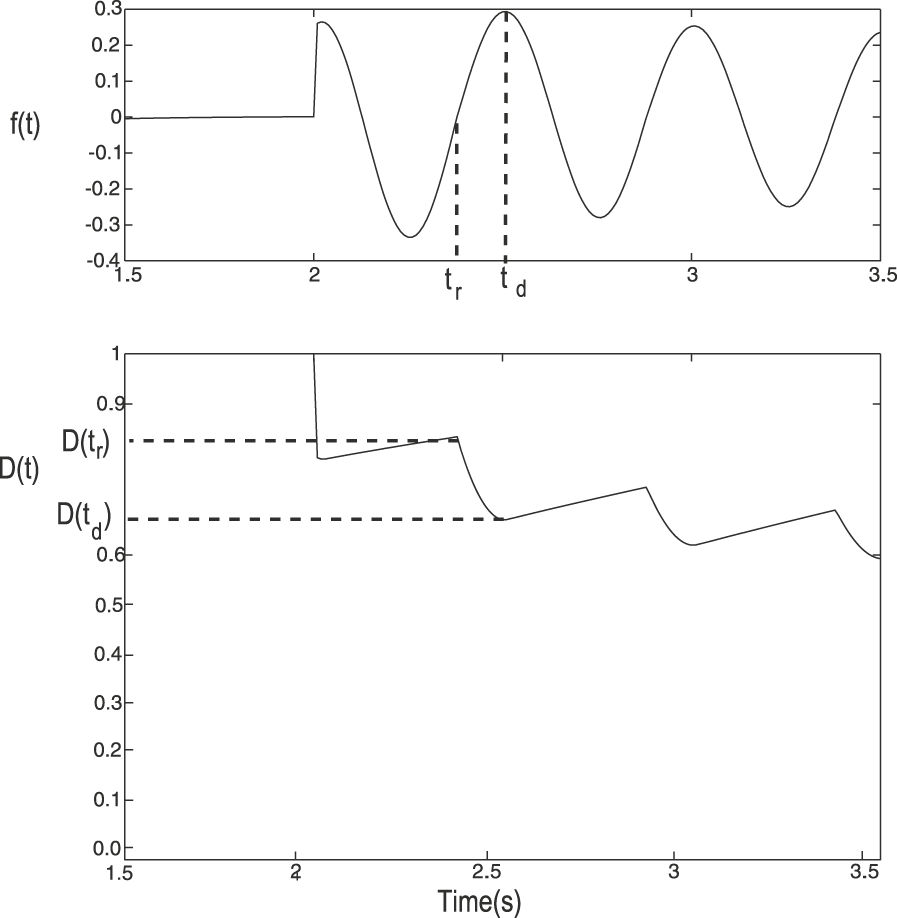
Based on the previous observations, we have developed a novel model for synaptic depression at the Tm1 synapses, which can be described as follows. Depression is implemented as a variable with values in the interval [0, 1], where a value of unity indicates no depression and a value of 0 indicates maximum depression. The depression factor multiplies the Tm1 activity to compute the postsynaptic response. Initially, the value of the depression factor is set to unity. During the time the cell response is rising and positive with respect to the resting potential, the depression factor decreases in value. While the cell response is decreasing or below the resting potential, the value of the depression factor is allowed to recover (towards unity). The postsynaptic effect of each cycle of activity in Tm1 is scaled down by the value of the depression factor at the beginning of the cycle. The decrease in the depression factor during rising responses is proportional to the amplitude of the rise.
Mathematically, let the Tm1 response (with the resting potential removed) be f (t). Let the time of the beginning of the rise of the last positive modulation in f (t) be called t r and the time when this response stops rising and starts decaying be t d (see Fig. 2). If D(t) represents the depression factor, which is initialized to a value of unity, and τ d the time constant of recovery, the model may be described as follows.

Illustration of model for depression in Tm1 synapses. The top plot shows f(t), the response of a simulated Tm1 (with resting potential removed) after stimulation with a sinusoidal grating moving at 2 Hz (contrast = 0.5). The time of the beginning of the rise of a positive modulation t r and the time the response begins to decay t d are indicated for one cycle. The bottom plot shows the depression factor D(t) for this stimulus. The levels of depression at the times t r and t d are marked on the plot. The depression factor becomes smaller (indicating greater depression) as the Tm1 value increases from resting and slowly recovers when Tm1 is not increasing. Multiple increases of Tm1 at sufficient frequency cause the depression factor to decline and stay at a low average level.

The postsynaptic response from Tm1 adjusted for depression (Tml d ) would thus be:

where V rest is the resting potential. Furthermore, if f(t) is a sinusoid of frequency f and amplitude A, then the magnitude of the scale factor D(t r) in each cycle n of f(t) can be described by the following nonlinear recursive equation:

where D(t
r) = 1 during the first cycle (n = 1). Note that depression recovers during three quarters of every cycle (when f(t) is decreasing or negative), hence the  factor in the exponent in eqn. (4). In order to maximize the depression elicited by f(t), one needs to minimize D(t
r), which can be accomplished by maximizing A or by maximizing the frequency f. Decreasing D(t
r) will, however, have the effect of decreasing the product A· D(t
r), which will decrease the maximum depression reached during the next cycle. Eventually, the reduction in the depression factor during a particular cycle will be fully recovered by the beginning of the next cycle, at which point D(t) approaches a steady-state value. This eventual approach of synaptic depression to a steady-state level is illustrated in Fig. 3, which shows the response of the Tm1 unit from the expanded neuronally based EMD model (refer to Fig. 1), the postsynaptic response adjusted for depression Tml
d
, and the depression factor D(t). Because in the neuronally based EMD model, all responses are with respect to a zero response level in the absence of stimulation (zero resting potential), subtraction of the resting response level is not necessary.
Synaptic depression in Tm1. Plots show the Tm1 response (top), the postsynaptic response to Tm1 input adjusted for depression Tml d (center) and the corresponding depression factor D(t) (bottom). The stimulus was a sinusoidal grating moving at a temporal frequency of 2 Hz (contrast = 0.5). The dashed traces in the Tml d plot show the envelope produced by the effect of the depression factor on the Tm1 response. Notice the asymptotic approach of depression to a steady-state level.

Note that this synaptic model is based on increasing depression only when the Tm1 response is rising above the resting potential. Because the model of Tm1 is symmetric in its response to positive and negative modulations with respect to a resting potential, the same results would have been produced if we had used the negative modulations to compute depression. Another possibility would be to increase depression whenever the response of the cell is increasing, regardless of whether the response is positive or negative with respect to the resting potential. Because of the symmetry in Tm1, this would only result in doubling A in eqn. (4) and in reducing the time of recovery to one half of a cycle. Reducing the time constant of recovery and using a scaled version of A would thus generate the same results as the model proposed. In addition, since the mean luminance is almost entirely removed from all input signals, all practical inputs will cause both positive and negative modulations of Tm1.
Contrast saturation through shunting inhibition
In previous versions of the neuronally based EMD model (Rivera-Alvidrez & Higgins, Reference Rivera-Alvidrez and Higgins2005), contrast saturation was implemented using saturating elements as in Egelhaaf and Borst (Reference Egelhaaf and Borst1989) and shunting inhibition used a simplified formula. These elements allowed insufficient degrees of freedom to match the shape of contrast saturation curves required by the present model (e.g., refer to Fig. 7), so saturating elements were removed, and instead, shunting inhibition was modeled using the biophysical equation outlined in Koch (Reference Koch1999):


where V
s is the output of the shunting synapse, Em
and gm
denote the potential and the conductance of the input, respectively, at location m,  denotes the transfer resistance between location m and n, and the subscripts e, i, and s denote the excitatory input location, inhibitory input location, and the soma location, respectively. Eqn. (5) not only accounts for the biophysics of shunting inhibition but also produces the nonlinearity of contrast saturation.
Materials and methods
Simulations were run using the Matlab software (The Mathworks, Natick, MA). The two-dimensional simulations incorporated a 100 × 100 pixel image viewed by a 20 × 20 hexagonal array of photoreceptors and an equal number of EMD models. The filters used in the model were implemented as first order with time constants of 250 ms for the high-pass filters, 150 ms for the first low-pass filters, and 50 ms for the final low-pass filters. The time step used for all simulations was 10 ms.
In every experiment, we used the neuronally based model shown in Fig. 1, which includes contrast and pattern size saturation. Contrast saturation was achieved through the use of eqn. (5), while LPTC integration of EMD inputs (also called “gain control”) was implemented as described in Borst et al. (Reference Borst, Egelhaaf and Haag1995) and Borst et al. (Reference Single, Haag and Borst1997) to produce pattern size saturation, with the output V of the G.C. block defined by:

where Ee and Ei are the excitatory and inhibitory reversal potentials, ge and gi are the excitatory and inhibitory conductances, and g leak is the leakage conductance. The values for Ee and Ei were set to 0.4 and −0.3, respectively, the same as the values used by Single et al. (Reference Single, Haag and Borst1997). The conductances ge and gi were driven by the sum of the outputs of the rectified T5 units responding to the simulated tangential cell’s preferred direction and the sum of the T5 units responding in the null direction, respectively (refer to “G.C.” block in Fig. 1). The value of the conductance g leak was empirically set to 3.5 S.
Adaptation was implemented as described in the previous section. The time constant of recovery τd
was set to 3.7 s. The adapting algorithm was implemented in the Tm1 synapses onto T5 and Tm9, as shown in the blocks labeled “A” in Fig. 1. Within the center-surround spatial filter [eqn. (1)], the first Gaussian filter g
1 had a σ
1 of 13 pixel units, while the second Gaussian filter g
2 had a σ
2 of 4 pixel units. These two values were chosen to match the spatial tuning intrinsic to the EMD model. The kernel size used for both filters was chosen to be 54 pixel units as the minimum to avoid significant artifacts in the filters. The relative weight w between these two filters was empirically set to be 0.98, in order to produce the desired amount of adaptation to wide-field flickering stimuli relative to the amount of adaptation to motion stimuli (see Fig. 7). In the shunting inhibition function [eqn. (5)],  ,
 ,
 ,
 ,
 ,
 , and Ee
were each empirically set to be 11, 65, 16, 15, 100, 16 MΩ, and 0.5 arbitrary voltage units, respectively, to match electrophysiological data (Koch, Reference Koch1999). Ei
was set to 0 to model a shunting inhibitory synapse. ge
and gi
were the rectified excitatory input and the rectified inhibitory input, respectively.
In our current model, the reduction in contrast sensitivity (as calculated in Harris et al., Reference Harris, O’Carroll and Laughlin2000) was quantitatively matched to that observed in real LPTCs by Harris et al. (Reference Harris, O’Carroll and Laughlin2000), by empirically adjusting the w parameter [amount of low spatial frequency attenuation in eqn. (1)] in the center-surround spatial filter and the τ d parameter [time constant of recovery in eqn. (2)] of the synaptic depression at the TM1 level. The value of w determined the difference in the amount of contrast sensitivity reduction between motion-adapted and flicker-adapted responses. The larger the value of w, the greater the amount of mean luminance that was removed from the input image, resulting in a smaller reduction in contrast sensitivity for flicker-adapted responses relative to motion-adapted responses. The value of τ d affected the amount of reduction in contrast sensitivity for motion-adapted responses, with a larger value of τ d producing a larger amount of reduction in contrast sensitivity.
The input to all simulations was a two-dimensional sinusoidal grating moving in the horizontal direction (the preferred direction of the EMD) with initial phase chosen randomly. The results of 10 simulations were averaged to obtain the model response, which was computed as the sum of the outputs of all units, ignoring fringe pixels, which were nonfunctional due to lack of neighbor interaction. The simulated tangential cell response was obtained by the rectification of the T5 outputs and subsequent subtraction of T5 units with opposite preferred directions, as discussed in Melano and Higgins (Reference Melano and Higgins2005) and shown in Fig. 1.
Results
Fig. 4a shows the simulated LPTC response to a square-wave grating, which moved at a constant speed for 3 s at different contrast levels after being adapted to a spatially uniform display at the mean luminance. Notice that the responses produced are both a function of the Tm1 depression rates and of contrast saturation. Contrast saturation tends to reduce the effect of adaptation at frequencies that elicit high response levels, as shown in the 2 Hz plots. Importantly, the effect of adaptation appears more pronounced for high-contrast high-frequency stimuli, as expected. Furthermore, as the frequency and the contrast are increased, the depression factor reaches smaller values (indicating more depression), a feature more clearly visible in Fig. 4b, which plots the time course of the depression factor D(t) for the same stimuli. All these features were previously observed in electrophysiological recordings of H1 LPTCs, as they responded to the same type of stimuli (compare with fig. 3 in Reisenman et al., Reference Reisenman, Haag and Borst2003). It should be noted that this is “adaptation” in a weak sense since much of this data can be reproduced with a standard EMD model (Egelhaaf & Borst, Reference Egelhaaf and Borst1989; Higgins et al., Reference Higgins, Douglass and Strausfeld2004).
Adaptation during continuous preferred direction motion stimulation. (a) Simulated tangential cell response to a square-wave grating moving at three different temporal frequencies and three contrast levels in the cell’s preferred direction. A uniform mean luminance stimulus was shown between presentations of moving stimuli. (b) Depression factor D(t) for the same stimuli. Increasing either the contrast or the temporal frequency of the visual stimulus reduces the values reached by D(t).

The responses of the model to motion stimuli moving in the null direction are shown in Fig. 5. Because the Tm1 cell is nondirectional, the features of adaptation are similarly produced with stimulation in the cell’s null direction, as desired. The rates of adaptation at the different contrast levels and temporal frequencies are in qualitative agreement with H1 recordings (compare to fig. 9 of Reisenman et al., Reference Reisenman, Haag and Borst2003). Note that the asymmetry in positive and negative response levels (comparing Figs. 4 and Reference Chance, Nelson and Abbott5) is due to the asymmetry in constants used in the gain control formula, eqn. (6).
Adaptation during continuous null direction motion stimulation. Simulated tangential cell response to a square-wave grating moving at three different temporal frequencies and three visual contrasts in the cell’s null direction. The stimulus was blanked to a uniform mean luminance level between presentations of moving stimuli. These stimuli are the same as those used by Reisenman et al. (Reference Reisenman, Haag and Borst2003), presented in that case to an H1 LPTC, and the results from the model are qualitatively quite similar to the cellular responses.

Adaptation in the model is directionally insensitive, as expected from the properties of Tm1. Fig. 6 shows the simulated LPTC response to a test stimulus before and after a period of strong adaptation with a high-frequency high-contrast grating moving in the preferred direction and in the antipreferred or null direction. Notice that the response to the second test stimulus is attenuated by the depression elicited by the adapting grating, similar to previous tangential cell recordings (compare to fig. 1 in Harris et al., Reference Harris, O’Carroll and Laughlin2000). Moreover, decreasing the frequency of the stimulus from 20 Hz during the adapting phase to 5 Hz during the second test phase increases the time that the depression has to recover during subsequent cycles. As a result, the Tm1 depression factor D(t) recuperates to a higher value during the test stimulus (see bottom plots in Fig. 6), which causes the response of the simulated LPTC to increase during the test phase. This increase has also been observed in LPTC recordings (Harris et al., Reference Harris, O’Carroll and Laughlin2000).
LPTC model response to a test grating (30% contrast, 5 Hz temporal frequency, indicated by the black bar) before and after strong motion adaptation with a sinusoidal grating (95% contrast, 20 Hz temporal frequency, indicated by the gray bar), which is moving (a) in the preferred direction and (b) in the antipreferred or null direction. Top plots show the simulated tangential cell response; bottom plots show the time course of the depression factor D(t). This is the same combination of stimuli presented to an HS LPTC by Harris et al. (Reference Harris, O’Carroll and Laughlin2000), and responses of the model (top two panels) are qualitatively quite similar to cellular responses.

Next, we tested adaptation with motion versus wide-field flicker (see Discussion about counterphase flicker). Fig. 7 shows the steady-state response of the model during the test stimulus before and after adaptation with wide-field flicker and with motion, as the contrast is increased. As done in Harris et al. (Reference Harris, O’Carroll and Laughlin2000), we evaluated the contrast that was required to elicit the 10 and 50% criterion response levels for each contrast response curve and determined the reduction in contrast sensitivity for each form of adaptation. We found that the preferred direction motion adaptation produced approximately a 3.5-fold reduction in contrast sensitivity (ΔCSgain,10% =3.48 and ΔCSgain,50% = 3.51), while the wide-field flicker produced approximately a 1.5-fold reduction in contrast sensitivity. These values matched closely with the results from recorded electrophysiological data when the effect of the afterpotential was removed.
Simulated LPTC responses from adaptation to motion versus adaptation to wide-field flicker. Preferred direction motion adaptation produced approximately a 3.5-fold reduction in contrast sensitivity (ΔCSgain,10% = 3.48 and ΔCSgain,50% = 3.51), while the wide-field flicker produced approximately a 1.5-fold reduction in contrast sensitivity. The horizontal dashed line shows the 50% response level, and the three vertical dashed lines show the contrast required to achieve 50% response in all three cases.

Fig. 8a shows the comparison between the contrast response curves from adaptation with motion in the preferred direction and adaptation with motion in the antipreferred direction. Motion in the antipreferred direction induced a 3.5-fold reduction in contrast sensitivity (ΔCSgain,10% =3.49 and ΔCSgain,50% = 3.50), comparable to the effect from adaptation to motion in the preferred direction.
Simulated LPTC responses from adaptation to motion in the preferred and antipreferred direction. Motion in the antipreferred direction induced a 3.5-fold reduction in contrast sensitivity (ΔCSgain,10% = 3.49 and ΔCSgain,50% = 3.50), the same as the effect from adaptation to motion in the preferred direction. Adaptation to motion in the orthogonal direction (data not shown) yielded a 3.5-fold reduction in contrast sensitivity (ΔCSgain,10% =3.55 and ΔCSgain,50% = 3.51), slightly more than the effect of adaptation to preferred direction motion. The simulated mean LPTC response was determined between 200 and 500 ms following the onset of the test stimulus (before and after adaptation).

Consistent with results from Harris et al. (Reference Harris, O’Carroll and Laughlin2000), adaptation to motion on average yielded a 3.5-fold reduction in contrast sensitivity regardless of the direction of motion. We further tested this by looking at the effect of adaptation to motion in the orthogonal direction (Fig. 8b). We found that adaptation to motion in the orthogonal direction yielded a 3.5-fold reduction in contrast sensitivity (ΔCSgain,10% =3.55 and ΔCSgain,50% = 3.51), comparable to the effect of adaptation to preferred direction motion.
Discussion
A neuronally based model of insect visual adaptation inspired by models of synaptic depression in mammalian vision cells was incorporated in the Tm1 synapses of the neuronally based EMD model. Even though the aim was to produce the simplest model that could enable us to compare the rough features of the simulation results with the electrophysiology, the results obtained match closely, in many cases, the time course followed by the cell’s response. Although our model does not attempt to address the afterpotential or output range reduction components of adaptation, both which are believed to originate in the tangential cell, it does encompass the strong temporal frequency dependence of adaptation, the asymptotic approach of adaptation to a steady-state level, and the observed recovery of LPTC responses from a strongly adapted state induced by a high-frequency high-contrast grating (refer to Fig. 6), all of which may be attributed to contrast gain reduction.
Contrast saturation from the implementation of the biophysical shunting inhibition at the level of T5 cells reduces the contrast dependence of the rates of adaptation in LPTC responses to sustained motion stimulation. While Maddess et al. (1985) reported a weak dependence of H1 adaptation rates during continued motion stimulation on contrast, high-contrast high-frequency gratings are found to induce strong adaptation based on the effect they have on a subsequent test stimulus (Harris et al., Reference Harris, O’Carroll and Laughlin2000). Our results show that even though adaptation is highly dependent on contrast, as shown in Fig. 4b, this dependence is obscured in the simulated cell responses by contrast saturation, which tends to reduce the effect of adaptation as the contrast is increased. Thus, while in some cases the responses to a moving grating at different contrast levels appear to simply be scaled versions of each other (e.g., refer to 10 Hz plots in Fig. 4a and 4b), the levels and rates of adaptation may be significantly affected by contrast (refer to Fig. 4b). Because adaptation in the model occurs before contrast saturation, this contrast dependency, though not evident in the cell’s response, will be reflected in the magnitude of the reduction of the cell’s response to a low-contrast test grating.
Synaptic depression may arise through post- or presynaptic conditions. Postsynaptic conditions may involve receptor desensitization (Takahashi et al., Reference Takahashi, Kovalchuck and Attwell1995), while presynaptic depression may arise from reduced efficacy of the release machinery or from depletion of releasable vesicles (Neher, Reference Neher1998). Because the properties of the Tm1 synapses or similar synapses in this part of the fly’s visual ganglia are largely unknown, we cannot distinguish between these possibilities. The large size and abundance of vesicle pools observed in the Tm1 synapses, however, make vesicle depletion an unlikely source of depression in Tm1 (Nicholas J. Strausfeld, U. Arizona, personal communication).
Adaptation in the current model occurs only when the Tm1 signal is positive with respect to the resting potential of the cell and increasing in value. Since the “resting potential” of the simulated cell is defined as the mean value of the signal, every signal has both positive and negative components, and thus, this adaptation algorithm works for any signal. Adaptation can alternatively be made to occur for negative and decreasing signals, or even in both cases previously mentioned, without qualitatively affecting the results (data not shown).
Adaptation with wide-field flicker in the current model was found to be weaker than adaptation with motion as observed in LPTC electrophysiological data. The implementation of the center-surround spatial filter preserved motion information in the input signals while attenuating the mean luminance from flickering stimuli. This allowed the simulated Tm1 cell, the locus of adaptation in the model, to respond more strongly to motion than to wide-field flicker. The reduction in sensitivity to flicker was quantitatively matched to that observed in real LPTCs by Harris et al. (Reference Harris, O’Carroll and Laughlin2000), by empirically adjusting the w parameter [imbalancing the two Gaussian spatial filters in eqn. (1)] in the center-surround spatial filter and the τ d parameter [time constant of recovery in eqn. (2)] of the synaptic depression at the TM1 level. The current model was also able to show that adaptation to motion in any direction, including the anti-preferred and the orthogonal directions, elicited simulated LPTC responses with comparable amounts of reduction in contrast gain, as observed by Harris et al. (Reference Harris, O’Carroll and Laughlin2000) in real LPTC responses. However, Harris et al. (Reference Harris, O’Carroll and Laughlin2000) showed that adaptation to a counterphase flickering grating, in which only local flicker is induced, was also weaker than adaptation to motion. Our model cannot currently explain this data; in fact, adaptation to counterphase flicker in our model is approximately equivalent to adaptation to motion (data not shown). Clearly, another mechanism is in play to reduce counterphase flicker adaptation responses, perhaps a more sophisticated motion detector at the Tm1 level than our current model incorporates.
Similarities between adaptation in fly interneurons and adaptation in mammalian neurons and human psychophysics have been previously noted (Harris et al., Reference Harris, O’Carroll and Laughlin2000). Our work suggests that the mechanism of adaptation through short-term synaptic depression may be common to insect tangential cells and to visual motion-sensitive neurons in the primary visual cortex of rats. How these two species could have arrived to the same neural principles may be explained in terms of evolutionary convergence, where unrelated species under similar environmental constraints independently arrive through evolution to the same computational solutions (Nishikawa, Reference Nishikawa2002).
Acknowledgments
This research was supported by grant number R01 RR008688-16A1 from the National Institutes of Health. The authors gratefully acknowledge the advice and assistance of Prof. Nicholas J. Strausfeld and Dr. John K. Douglass of the Department of Neuroscience at the University of Arizona and the work of Dr. Lise A. Johnson on the shunting inhibition model.