Energy exchanges in the flow past a cylinder with a leeward control rod

Neelakash Biswas; Murilo M. Cicolin; Oliver R.H. Buxton

doi:10.1017/jfm.2022.297

Energy exchanges in the flow past a cylinder with a leeward control rod

Published online by Cambridge University Press: 03 May 2022

and

Neelakash Biswas*: Affiliation:
Department of Aeronautics, Imperial College London, London SW7 2AZ, UK
Murilo M. Cicolin: Affiliation:
Department of Aeronautics, Imperial College London, London SW7 2AZ, UKEscola Politécnica, University of São Paulo, Brazil
Oliver R.H. Buxton: Affiliation:
Department of Aeronautics, Imperial College London, London SW7 2AZ, UK
*: †Email address for correspondence: n.biswas20@imperial.ac.uk

Article contents

Abstract
Introduction
The data set
Mean flow properties
Dominant frequencies in the flow field
Multiscale triple decomposition: extraction of coherent structures
Energy budget equations
Summarising the energy cascade
Conclusion
References

Rights & Permissions

Abstract

We study the energy exchanges between coherent structures and the mean flow in the wake of a cylinder in the presence of a leeward control rod using particle image velocimetry data at Reynolds number ($Re$) $20\times 10^3$. The shedding of the control rod depends on the oncoming shear layer and hence the downstream interaction of the main cylinder's and control rod's wake strongly depends on the control rod's setting angle ($\theta$). In this work we study this interaction between the shedding modes from the cylinder and control rod at different $\theta$. New secondary coherent motions with distinct characteristic frequencies appear in the flow field aside from the frequencies associated with the sheddings of the control rod, the main cylinder and its harmonics. A multiscale triple decomposition method is applied to extract the coherent modes associated with each of these frequencies, and the dynamics of the modes are studied using kinetic energy budget equations. The primary shedding modes of the control rod and main cylinder, as well as the harmonics of the main cylinder's shedding modes, are found to be primarily energised by the mean flow at this $Re$, while the secondary modes are almost entirely energised by the primary modes, similar to the findings of Baj & Buxton (Phys. Rev. Fluids, vol. 2, issue 11, 2017, 114607) for a different multiscale flow configuration. The remarkable similarity in the energy exchange process forming the secondary coherent modes, observed in two different studies, hints at a possible universality in the formation process of these secondary structures in a multiscale flow.

JFM classification

Wakes/Jets: Wakes Wakes/Jets: Vortex streets

Information

Type: JFM Papers
Information: Journal of Fluid Mechanics , Volume 941 , 25 June 2022, A36
DOI: https://doi.org/10.1017/jfm.2022.297 [Opens in a new window]
Copyright: © The Author(s), 2022. Published by Cambridge University Press

1. Introduction

Flow past a circular cylinder has been a canonical problem in fluid dynamics for decades, demonstrating a multitude of physics from the onset of instability and vortex shedding (Monkewitz & Nguyen Reference Monkewitz and Nguyen1987; Yang & Zebib Reference Yang and Zebib1989) to the transition to a fully turbulent wake (Zhang et al. Reference Zhang, Fey, Noack, König and Eckelmann1995; Williamson Reference Williamson1996). The flow is known to be primarily governed by the Reynolds number ($Re$), usually defined based on the cylinder's diameter $D$ and free stream velocity $U_{\infty }$. The flow remains steady and symmetric until a critical $Re$ which depends on several factors such as the cylinder's aspect ratio, blockage ratio and free stream turbulence level (Strykowski & Sreenivasan Reference Strykowski and Sreenivasan1990; Sengupta, Singh & Suman Reference Sengupta, Singh and Suman2010). Beyond the critical $Re$, the well known unsteady, time periodic von Kármán vortex street is formed producing fluctuating loads on the cylinder which can be harmful for a variety of engineering structures exposed to strong winds/currents. Several strategies have therefore been undertaken to control or modify the vortex shedding process and hence reduce the fluctuating loads. A review of the different control strategies that have been used to control a cylinder wake can be found in Choi, Jeon & Kim (Reference Choi, Jeon and Kim2008). Amongst them, one strategy is to put a control cylinder, commonly termed as a control rod, in the vicinity of the shear layer separating from the main cylinder, which was first studied by Strykowski & Sreenivasan (Reference Strykowski and Sreenivasan1990). The authors reported complete suppression of vortex shedding up to $Re\approx 90$ for a cylinder with length-to-diameter ratio of 15. Motivated by these results, a series of investigations were performed to quantify the drag reduction by placing a control rod over a wide range of $Re$ through experiments (Sakamoto & Haniu Reference Sakamoto and Haniu1994; Bingham, Morton & Martinuzzi Reference Bingham, Morton and Martinuzzi2018; Cicolin et al. Reference Cicolin, Buxton, Assi and Bearman2021) and numerical simulations (Mittal & Raghuvanshi Reference Mittal and Raghuvanshi2001; Dipankar, Sengupta & Talla Reference Dipankar, Sengupta and Talla2007). In addition to the drag reduction, a number of different flow states were identified depending on the precise position of the control rod relative to the main cylinder (Parezanović & Cadot Reference Parezanović and Cadot2012; Cicolin et al. Reference Cicolin, Buxton, Assi and Bearman2021). These flow states can be characterised by the velocity signal between the cylinder and the rod, which are related to different coherent structures in the system's wake (Cicolin et al. Reference Cicolin, Buxton, Assi and Bearman2021). Unlike previous studies, where modification of the forces acting on the main cylinder have been the key area of interest, we focus on the energy exchanges taking place in the wake of the system characteristic of state I, for $90^\circ \leq \theta \leq 115^\circ$, as identified by Cicolin et al. (Reference Cicolin, Buxton, Assi and Bearman2021). Although this is not the most favourable state regarding control, this type of multiscale flow is very common in engineering applications, and this analysis yields deeper insights into the formation and mutual interaction of different coherent structures introduced into the flow by the presence of the rod and how they influence the overall development of the system's wake.

Flow past a cylinder in the presence of a control rod can contain multiple length/time scales introduced by the main cylinder and the control rod. When the position of the control rod enables both the main cylinder and the rod to form distinct wakes, an interaction between the two wakes can result in the formation of new coherent structures with their own characteristic frequencies, as reported by Baj & Buxton (Reference Baj and Buxton2017). In fact Cicolin et al. (Reference Cicolin, Buxton, Assi and Bearman2021) recently reported the observation of two such new frequencies, aside from those associated with the sheddings of the main cylinder and the control rod, for a range of positions of the control rod with respect to the main cylinder. These frequencies exactly corresponded to the sum and difference of the frequencies associated with the fundamental shedding modes of the main cylinder and control rod. In the present manuscript we use the same data set as Cicolin et al. (Reference Cicolin, Buxton, Assi and Bearman2021) and develop a deeper understanding of the formation of these new frequencies and their role in the overall energy cascade process in the combined system's wake. We also quantify the roles played by the harmonics of the main cylinder's shedding mode, which are commonly identified in the wake behind a cylinder and are found to be energetic enough to influence the overall energy cascade (Parezanović, Monchaux & Cadot Reference Parezanović, Monchaux and Cadot2015; Jin, Symon & Illingworth Reference Jin, Symon and Illingworth2021). As we wish to assess the energy budgets of each of these modes individually, as a first step we need an efficient tool to distinguish these modes from the mean flow and the incoherent background turbulence (or stochastic velocity fluctuations). Hussain & Reynolds (Reference Hussain and Reynolds1970) first introduced a triple decomposition method to extract the coherent/periodic part of a flow from the mean and stochastic component based on a known phase reference. Here the velocity field was decomposed as

(1.1)

\begin{equation} u(x,t) = \bar{u}(x,t) + \tilde{u}(x,t) + u^{''}(x,t), \end{equation}

where, $\bar {u}(x,t)$ is the mean component, $u^{''}(x,t)$ corresponds to the stochastic component and $\tilde {u}(x,t)$ corresponds to the coherent component of the velocity. Hussain & Reynolds (Reference Hussain and Reynolds1970) considered a channel flow perturbed by an oscillating ribbon, however, triple decomposition of the form presented in (1.1) has also been successfully applied to free shear flows (e.g. that past a cylinder (Cantwell & Coles Reference Cantwell and Coles1983)) and wavy/moving surfaces (Sengupta & Lekoudis Reference Sengupta and Lekoudis1985; Lekoudis & Sengupta Reference Lekoudis and Sengupta1986). But, when there are multiple scales in the flow, multiscale triple decomposition is not a trivial extension of that proposed by Hussain & Reynolds (Reference Hussain and Reynolds1970). Baj, Bruce & Buxton (Reference Baj, Bruce and Buxton2015) first proposed an extension of the triple decomposition method to multiscale flows that was successfully applied to extract individual coherent modes in a multiscale flow (Baj & Buxton Reference Baj and Buxton2017) without the need for a phase reference. Here the total velocity is represented as the combination of a mean component ($\bar {u}(x,t)$), a stochastic component ($u^{''}(x,t)$) and a sum of velocity modes corresponding to individual coherent structures ($\tilde {u}_l(x,t)$) as follows:

(1.2)

\begin{equation} u(x,t) = \bar{u}(x,t) + \sum_l\tilde{u}_l(x,t) + u^{''}(x,t). \end{equation}

We use the same methodology to extract the different coherent modes present in the current flow. The kinetic energy budgets of each of the modes and also the mean flow is then obtained using the multiscale triple-decomposed kinetic energy budget equations derived by Baj & Buxton (Reference Baj and Buxton2017). Three observations of the present study are noteworthy. (1) The mean kinetic energy budget terms for the bare cylinder and the cylinder with a control rod reveal significant differences and the differences correlate well with the variation of drag forces reported by Cicolin et al. (Reference Cicolin, Buxton, Assi and Bearman2021). (2) There exist fundamental differences in the way the different coherent structures in the flow are formed and in the way that they interact with each other. (3) Alongside conventional energy transfers from low frequencies to high frequencies, there exists a significant amount of nonlinear energy transfer from high frequencies to low frequencies.

The paper is organised in the following way. In § 2 we briefly explain the data set used in the present work. Section 3 discusses the variation of the mean flow properties in the presence of the control rod. In § 4 the dominant frequencies present in the flow field are identified. In § 5 we discuss the multiscale triple decomposition method utilised to extract the coherent motions from the flow field. In § 6 we briefly discuss the turbulent kinetic energy (TKE) budget equations we use for the analysis. The budgets for the mean flow and the coherent fluctuations are also reported in this section. Finally, we comment on the overall energy exchange process within the combined system's wake in § 7 followed by concluding remarks in the final section.

2. The data set

The present manuscript utilises the particle image velocimetry (PIV) data set originally obtained by Cicolin et al. (Reference Cicolin, Buxton, Assi and Bearman2021). The flow field consists of a main cylinder of diameter ($D$) 0.05 m with a control rod of diameter $d=0.1D$ mounted at a radial position ($R$) of $0.7D$ giving a gap of $0.15D$ between the cylinder and the control rod. A schematic of the main cylinder and control rod assembly is shown in figure 1. The free stream velocity ($U_{\infty }$) is fixed at $0.4\,{\rm m}\,{\rm s}^{-1}$ giving a Reynolds number $Re_D=20 \times 10^3$ for the cylinder and $Re_d = 2\times 10^3$ for the control rod. The PIV measurements were conducted in the midsectional plane of the cylinder–control rod assembly. Cicolin et al. 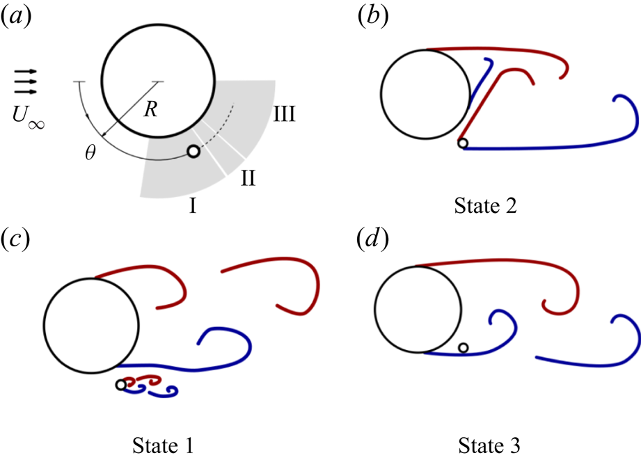(Reference Cicolin, Buxton, Assi and Bearman2021) varied the control rod angle ($\theta$) between $90^\circ$ and $140^\circ$ and reported three flow states, alongside a bistable flow state. Qualitative representations of the flow states are shown in figure 2. In state I, i.e. $90^\circ \leq \theta \leq 115^\circ$, the main cylinder and the control rod form their own individual wakes. As the main motivation of the present manuscript is to understand the interaction between the distinct wakes of the cylinder and the control rod, we only focus on state I. The data used in the present manuscript is obtained at an acquisition frequency of 70 Hz, and the total acquisition time is around 42.86 s (a total of 3000 snapshots) which is close to 70 and 840 cycles of the main cylinder and control rod shedding, respectively. The spatial resolution of the experiments, $\delta _x$, is approximately $1.88\,{\rm mm} = 0.037D$. This spatial resolution is verified to be sufficient to resolve the coherent structures produced from the control rod (see Appendix B). Readers are referred to Cicolin et al. (Reference Cicolin, Buxton, Assi and Bearman2021) for further details on the data set and the experimental methodology employed to acquire it.

Figure 1.

A schematic of the main cylinder and control rod assembly.

Figure 2.

Flow states adopted from Cicolin et al. (Reference Cicolin, Buxton, Assi and Bearman2021) for the flow past a circular cylinder and a control rod in the range $\theta =90^\circ \text {--}180^\circ$ and for a fixed radial position $R'/D=0.7$. State I occurs for $90^\circ \leq \theta \leq 115^\circ$, state II for $120^\circ \leq \theta \leq 125^\circ$ and state III for $135^\circ \leq \theta \leq 180^\circ$. At $\theta =130^\circ$ the flow develops a bistability between states II and III.

3. Mean flow properties

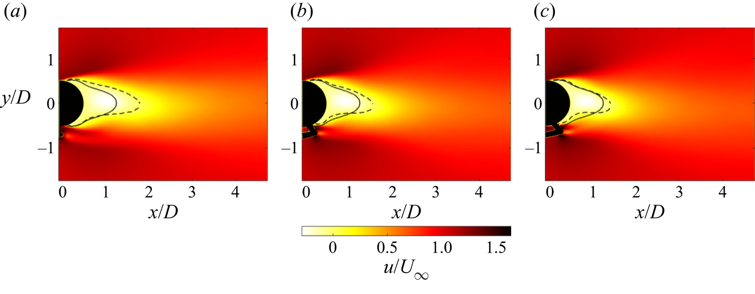
Let us first characterise the mean quantities of the flow field under investigation for different control rod positions ($\theta$) in state I. The variation of the mean streamwise velocity field with $\theta$ is shown in figure 3(a–c). As discussed previously, both the main cylinder and the control rod form distinct wakes. The large recirculating region behind the main cylinder is evident from the region of negative mean streamwise velocity. The wake of the control rod appears to be slightly deflected downwards due to a biased gap flow (Alam, Moriya & Sakamoto Reference Alam, Moriya and Sakamoto2003; Song, Lu & Kuo Reference Song, Lu and Kuo2013) between the control rod and the main cylinder. Similar wake deflections of small and medium rectangular prisms adjacent to another large rectangular prism have been reported by Baj & Buxton (Reference Baj and Buxton2017). In spite of the broadly similar wake structure at different $\theta$, subtle differences can be seen as $\theta$ is varied. To facilitate the differences, we estimate the extent of the recirculation region defined as $x:\bar {U}(x)=0$ ($\bar {U}$ being the mean streamwise velocity component), as shown by the dashed lines for different values of $\theta$. For comparison, the same for the bare cylinder is also shown as a solid line. At first glance, the recirculation region of the main cylinder wake with a control rod appears elongated compared with the bare cylinder at all control rod angles considered, an observation also reported in previous studies (Dalton, Xu & Owen Reference Dalton, Xu and Owen2001; Bingham et al. Reference Bingham, Morton and Martinuzzi2018). Dalton et al. (Reference Dalton, Xu and Owen2001) reported that in the presence of a control rod, the vortex shedding from the main cylinder was shifted slightly downstream, plausibly explaining the longer extent of the recirculation region observed. Also note from figure 3 that the streamwise extent of the recirculation region decreases with increasing $\theta$ similar to the observation of Dalton et al. (Reference Dalton, Xu and Owen2001). This shortening of the main cylinder's wake at higher $\theta$ is instrumental for the scope of the present manuscript as it translates to the fact that increasing $\theta$ slightly, changes the location where the wakes interact, which in turn changes the dynamics of the interaction significantly.

Figure 3.

Mean streamwise velocity field for (a) $\theta =90^{\circ }$, (b) $\theta =110^{\circ }$ and (c) $\theta =115^{\circ }$. The dashed lines depict the extent of the recirculation region for the main cylinder wake in the presence of a control rod, whilst the solid line represents the same for a bare cylinder.

To quantify the location of the wake interaction, we define wake intersection points as the locations where the root mean square (r.m.s.) transverse velocity fluctuation field ($v_{rms}$) forms a saddle, similarly to Baj & Buxton (Reference Baj and Buxton2017). Note that wake intersection points have been found to be an important parameter in multiscale generated turbulence (Mazellier & Vassilicos Reference Mazellier and Vassilicos2010; Gomes-Fernandes, Ganapathisubramani & Vassilicos Reference Gomes-Fernandes, Ganapathisubramani and Vassilicos2012). Mazellier & Vassilicos (Reference Mazellier and Vassilicos2010) showed that the downstream evolution of turbulence statistics scales with the wake intersection length scale for the fractal grids tested. Further, wake intersection points were found to be important in the space scale unfolding (SSU) mechanism first proposed by Laizet & Vassilicos (Reference Laizet and Vassilicos2012) which yields an enhanced scalar transport in multiscale flows (Laizet & Vassilicos Reference Laizet and Vassilicos2012; Baj & Buxton Reference Baj and Buxton2019)

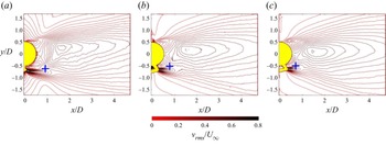
Figure 4(a–c) show the normalised $v_{rms}$ field for different $\theta$. The wake intersection points are shown as a (blue) + sign. The shortening of the main cylinder's wake at larger $\theta$ results in an earlier interaction between the two wakes, which is evident from the wake intersection points moving closer to the cylinder–control rod assembly with increasing $\theta$. The streamwise position of the wake intersection points are found to be around $x/D = 0.97,0.76$ and $0.72$ for $\theta = 90^\circ, 110^\circ$ and $115^\circ$, respectively.

Figure 4.

Normalised $v_{rms}$ field for (a) $\theta =90^\circ$, (b) $\theta =110^\circ$ and (c) $\theta =115^\circ$.

4. Dominant frequencies in the flow field

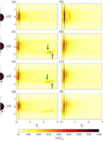
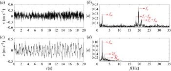
In order to identify the frequencies of importance we first present the evolution of the transverse velocity spectra in figure 5 for different $\theta$, at two streamwise positions $x/D=1$ and $x/D=2$. Time series of transverse velocity and corresponding fast Fourier transforms (FFTs) at some specific locations of interest are also shown as an example in Appendix D. In figure 5 we compare the evolution of the transverse velocity spectra for different $\theta$ with the bare cylinder. Figure 5(a) shows the spectrum for the bare cylinder at $x/D=1$. A strong peak can be seen at Strouhal number ($S_t = fD/U_{\infty }$) around 0.195 (corresponding frequency, $f_b \approx 1.56\,{\rm Hz}$) that correlates well with $S_t$ reported in the literature for vortex shedding behind a cylinder at high subcritical Reynolds numbers (Roshko Reference Roshko1961; Prasad & Williamson Reference Prasad and Williamson1997). When a control rod is placed at $\theta =90^\circ$, the intensity of the main cylinder's shedding mode drops slightly (see figure 5c) at $x/D=1$. Further, the Strouhal number reduces to $0.166$ (corresponding frequency, $f_m \approx 1.3\,{\rm Hz}$), which is around $15\,\%$ smaller than the bare cylinder's Strouhal number. Note that such a reduction in the frequency of the main cylinder in the presence of a control rod, or in general another cylinder of comparable diameter, has been reported in the past (Bearman & Wadcock Reference Bearman and Wadcock1973; Strykowski & Sreenivasan Reference Strykowski and Sreenivasan1990; Alam et al. Reference Alam, Moriya and Sakamoto2003; Parezanović & Cadot Reference Parezanović and Cadot2012; Song et al. Reference Song, Lu and Kuo2013). In fact, Parezanović & Cadot (Reference Parezanović and Cadot2012) reported a drop of around $15\,\%$ in the shedding frequency when a control rod of a similar size to the present study was placed at a similar radial and azimuthal position. However, the authors did not report the Strouhal number of the control rod shedding mode for the configuration. We observe a strong peak at $S_t=2.45$ (corresponding frequency, $f_c \approx 19.6\,{\rm Hz}$) in figure 5(c) which corresponds to the fundamental shedding mode of the control rod. If $S_t$ is calculated based on the control rod diameter $d$ instead of main cylinder diameter $D$, then the Strouhal number of the control rod shedding mode comes to around $0.245$. Note that this Strouhal number is higher than is typical for a bare cylinder at the control rod-based Reynolds number 2000 (Prasad & Williamson Reference Prasad and Williamson1997) as the shedding frequency can be a strong function of the shear of the oncoming flow. Such an increase in the control rod's shedding mode's frequency was also reported by previous studies on two side-by-side cylinders (Bearman & Wadcock Reference Bearman and Wadcock1973; Alam et al. Reference Alam, Moriya and Sakamoto2003; Song et al. Reference Song, Lu and Kuo2013) who found that a decrease in the frequency of one cylinder was associated with an increase in the other (smaller) cylinder's frequency. However, note that the streamwise velocity upstream of the control rod is higher than $U_{\infty }$ due to the acceleration of the flow past the cylinder. Hence, the actual Strouhal number of the control rod's shedding mode could be lower than the estimated value if the approach velocity is used to calculate the Strouhal number instead of $U_{\infty }$.

Figure 5.

Frequency spectra of the transverse velocity fluctuation at (a,c,e,g) $x/D=1$ and (b,d,f,h) $x/D=2$ for the (a,b) bare cylinder, (c,d) $\theta =90^\circ$, (e,f)$~\theta =110^\circ$ and (g,h)$~\theta =115^\circ$. Here $S_t$ is the Strouhal number calculated based on the main cylinder's diameter ($D$) and the free stream velocity ($U_{\infty }$).

Interestingly, around the frequency of the control rod's shedding mode, two additional prominent peaks are observed (indicated by green arrows) which correspond to the frequencies $f_c\pm f_m$. These two frequencies are believed to be generated by nonlinear interaction between the main cylinder's and control rod's fundamental frequencies. Whether the modes associated with these two frequencies can be termed ‘secondary modes’ will be justified in § 6. Nevertheless, for now let us term these as secondary modes until such a justification is presented. Note that the appearance of secondary frequencies in the wake of a two-circular-cylinder system of unequal yet comparable diameters has been reported in the past (Lam, Wong & Ko Reference Lam, Wong and Ko1993; Song et al. Reference Song, Lu and Kuo2013), but they have not been given much attention until recently (Baj & Buxton Reference Baj and Buxton2017, Reference Baj and Buxton2019; Cicolin et al. Reference Cicolin, Buxton, Assi and Bearman2021). In the work by Lam et al. (Reference Lam, Wong and Ko1993), the secondary frequencies were found to appear in the vicinity of the smaller cylinder wake (see figure 6 of Lam et al. (Reference Lam, Wong and Ko1993)) which is similar to our observation. Further, we note that the higher secondary mode ($f_c+f_m$) is located near the separated shear layer between the main cylinder and the control rod whereas, the lower secondary mode ($f_c-f_m$) resides more towards the opposite separated shear layer of the control rod. Baj & Buxton (Reference Baj and Buxton2017) recently studied the flow past a multiscale array of rectangular prisms and found exactly the same spatial configuration of secondary modes. This similarity in the spatial organisation of the secondary modes in $f-y$ space ($f$ being frequency and $y$ being transverse distance) in two very different classes of flow, is a remarkable finding and hints at a possible universality in their process of generation.

As we increase $\theta$ to $110^\circ$, the main cylinder's and the control rod's shedding frequencies remain almost the same as for $\theta =90^\circ$. We still observe the secondary modes at precisely the same combination of frequencies but their intensity (as well as that of the control rod's shedding mode) drops at $x/D=1$. Finally, the spectral signature of the secondary modes almost disappears at $\theta =115^\circ$ at $x/D=1$. This reduction of the intensity of the control rod's shedding mode at higher $\theta$ can be expected, as the control rod gets closer to the separated shear layer from the main cylinder at a higher $\theta$, thus facing a reduced oncoming flow velocity. In addition to that, if the rod approaches the separated shear layer, there is limited space and time for the control rods’ vortex street to develop before interacting with the main cylinder's wake. Considering these two effects, the shedding modes for the rod at $\theta =115^\circ$ are expected to be the weakest among all the currently considered cases. We also point out that the wake formed with the rod at $\theta =115^\circ$ is on the verge of changing from flow state I to II (see figure 2), where the control rod does not present its own vortex street with a distinct frequency. As we move to $x/D=2$, the spectral signature of the control rod's shedding and the secondary modes disappears for all control rod angles considered and the harmonics of the main cylinder's shedding mode ($f_m$) become important. These harmonics have been commonly observed in several other studies as well (Parezanović & Cadot Reference Parezanović and Cadot2012; Parezanović et al. Reference Parezanović, Monchaux and Cadot2015; Jin et al. Reference Jin, Symon and Illingworth2021). It might be possible to observe traces of even higher harmonics at farther downstream distances, but we only focus on the first two harmonics as most of the energy is contained in them (Jin et al. Reference Jin, Symon and Illingworth2021). For the rest of the paper we shall focus on $\theta =90^\circ$ and $\theta =110^\circ$, as the secondary frequencies were prominent for these two cases only.

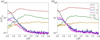
To quantify the spatial extent and relative strength of the modes we obtain the amplitude of the spectra of the transverse velocity of the various modes at different spatial locations. The spatial evolution of the spectral peaks of the transverse velocity of all the frequencies of interest is shown in figure 6 for $\theta =90^\circ$ and $110^\circ$. Figure 6 reveals a qualitatively similar picture for $\theta =90^\circ$ and $110^\circ$. Note that close to the main cylinder, at $x/D \approx 0.5$, the amplitudes of $f_c$ and $f_m$ are comparable to each other but $f_c$ quickly falls off as streamwise distance is increased. At $x/D \approx 0.5$, the secondary modes are significantly weaker compared with $f_c$ and $f_m$ and their amplitudes are significant only up to $x/D \approx 1.5$. The short spatial persistence of the secondary modes might explain why they were not observed in many previous experimental studies with similar control rod size to the present case. For instance, Parezanović & Cadot (Reference Parezanović and Cadot2012) obtained a frequency spectrum of the flow field at a fixed streamwise distance of $6D$, whilst Parezanović et al. (Reference Parezanović, Monchaux and Cadot2015) probed data at $x/D=1.5$ hence, it is not surprising that the spectral signature of the secondary modes was not captured in previous studies. Moreover, the bulk of the previous studies on a cylinder with a control rod have been performed at relatively low Reynolds numbers (Strykowski & Sreenivasan Reference Strykowski and Sreenivasan1990; Mittal & Raghuvanshi Reference Mittal and Raghuvanshi2001; Yildirim, Rindt & Steenhoven Reference Yildirim, Rindt and Steenhoven2010) where vortex shedding from the control rod does not initiate at all. At $\theta =90^\circ$, a clear dominance of the lower secondary mode ($f_c-f_m$) can be seen over the higher secondary mode ($f_c+f_m$). This observation correlates well with the observations of Baj & Buxton (Reference Baj and Buxton2017), who found that the low-frequency secondary modes were more spatially persistent than their high-frequency counterparts. Although $f_c-f_m$ has a lower amplitude than $f_c+f_m$ for $\theta =110^\circ$ at $x/D < 1$, $f_c-f_m$ does remain more persistent. Unlike $f_c$ and the secondary modes, the amplitudes of $f_m$ and its harmonics grow with streamwise distance. Now $f_m$ reaches its peak at $x/D \approx 1.5$ for both values of $\theta$, which correlates well with the streamwise location of maximum turbulence intensity reported by Cicolin et al. (Reference Cicolin, Buxton, Assi and Bearman2021). However, note that the amplitude of the main cylinder's shedding mode is almost twice as large for $\theta =110^\circ$ compared with $\theta =90^\circ$. This observation ties well with the reduced fluctuating forces observed for $\theta =90^\circ$ compared with $\theta =110^{\circ }$ (Cicolin et al. Reference Cicolin, Buxton, Assi and Bearman2021). In the next sections we identify the spatiotemporal structure of the modes associated with each of the frequencies discussed above and comment on their formation, relative strength, spatial extent and mutual interaction using TKE budget equations.

Figure 6.

Streamwise evolution of the maximum normalised spectral peak of the transverse velocity associated with different modes for (a) $\theta =90^\circ$ and (b) $\theta =110^\circ$.

5. Multiscale triple decomposition: extraction of coherent structures

As we have already shown, the near field of the flow ($x/D \lesssim 2$) contains several different coherent structures of perceptible amplitudes. To understand the dynamics of the modes we need to distinguish each of them from the mean and stochastic component of the flow, hence we need to use a triple decomposition technique similar to the one originally proposed by Hussain & Reynolds (Reference Hussain and Reynolds1970). The authors used conditional sampling based on a known reference signal to differentiate the coherent motion from the mean part and stochastic fluctuations. Baj et al. (Reference Baj, Bruce and Buxton2015) proposed a triple decomposition technique that can further distinguish between different coherent structures present in the flow without any prior knowledge of the modes or any need for a reference signal. The authors decomposed the flow field as the combination of a mean component ($\bar {u}$), sum of contributions from different coherent motions ($\tilde {u}_l$) and the incoherent or stochastic part ($u''$) as follows:

(5.1)

\begin{equation} u(x,y,t) = \bar{u}(x,y) + \sum_l \tilde{u}_l(x,y,t) + u^{''}(x,y,t), \end{equation}

where, $\tilde {u}_l$ corresponds to the velocity field of $l$th coherent motion. The spatial velocity fields associated with the coherent motions ($\tilde {u}_l(x,y)$) are obtained by using optimal mode decomposition (OMD), first proposed by Wynn et al. (Reference Wynn, Pearson, Ganapathisubramani and Goulart2013). The OMD algorithm is a generalised version of the dynamic mode decomposition (DMD) algorithm proposed by Schmid (Reference Schmid2010) and can identify individual coherent motions in the flow field under investigation. As the flow field is real valued, the OMD modes are either real or appear in a complex conjugate pair, say $\phi _{OMD}$ and $\phi ^T_{OMD}$. The spatiotemporal velocity field associated with a mode is then obtained by a linear combination of $\phi _{OMD}$ and $\phi ^T_{OMD}$, both multiplied by the associated time varying complex coefficients (see Baj et al. (Reference Baj, Bruce and Buxton2015) and Baj & Buxton (Reference Baj and Buxton2017) for details). The coefficients are obtained by projecting $\phi _{OMD}$ and $\phi ^T_{OMD}$ onto the snapshots of the flow field and it is worth noting that the projection method is not trivial. For the present problem in particular, where there are coherent motions quite closely spaced in the frequency domain (see the control rod's shedding mode and secondary modes in figure 5c,e), projecting the snapshots to a single mode corrupted the spectrum of the coefficient with the spectral signature of other closely spaced modes. The issue could be resolved by projecting onto all of the modes of physical relevance to the snapshots simultaneously. Finally, the coefficients are filtered using a bandpass filter similar to Baj et al. (Reference Baj, Bruce and Buxton2015). Baj et al. (Reference Baj, Bruce and Buxton2015) also compared the performance of OMD with proper orthogonal decomposition (POD) which has also been extensively used to extract coherent modes (Berkooz, Holmes & Lumley Reference Berkooz, Holmes and Lumley1993; Dipankar et al. Reference Dipankar, Sengupta and Talla2007). The authors found that POD was incapable of correctly identifying the mode shapes farther downstream from a multiscale wake-generating body, while OMD could identify the modes correctly. Although for the present analysis OMD and POD produce similar mode shapes, to be consistent with our previously published work we utilise OMD to perform the multiscale triple decomposition.

5.1. Extraction of primary coherent structures

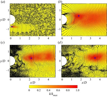
The multiscale triple decomposition technique using OMD is successfully applied to the present data set to obtain the coherent motions associated with the sheddings of the main cylinder and the control rod and also the harmonics of the main cylinder. The modes can be clearly identified as the least damped modes in the OMD spectra shown for $\theta =90^\circ$ and $110^\circ$ in Appendix A. Hussain (Reference Hussain1986) defined a coherent structure as a connected turbulent fluid mass of phase-correlated vorticity (hence velocity). We follow the same ideology to represent the coherent structures identified in the flow. In figure 7 we show the modes associated with $f_c$, $f_m$ and its harmonics for the case $\theta =90^\circ$. The filled contours show the time-averaged kinetic energies (defined as $(\overline {\tilde {u}_l\tilde {u}_l+\tilde {v}_l\tilde {v}_l})/2$) of the modes, while the contour lines represent the isophase lines of transverse velocity component obtained from complex $\phi _{OMD}$ for each of the modes. The isophase lines are shown from $-{\rm \pi}$ to ${\rm \pi}$ at steps decreasing with the frequency of the modes so that the spatial separation of the lines remains more or less the same for the different modes.

Figure 7.

Modes associated with (a) control rod shedding frequency and (b) cylinder shedding frequency at $\theta = 90^\circ$. Panels (c,d) show the second and third harmonics of the main cylinder shedding mode, respectively. The filled contour shows the energy of the modes while the contour lines represent isophase lines of transverse velocity fluctuation of the modes. The contour lines are shown from $-{\rm \pi}$ to ${\rm \pi}$ at step size (a) ${\rm \pi} /2$, (b) ${\rm \pi} /15$, (c) ${\rm \pi} /10$ and (d) ${\rm \pi} /7$. The (blue) + sign shows the location where the kinetic energies of the modes attain a maximum.

For the mode shown in figure 7(a), the isophase lines show a localised phase-correlated region in the vicinity of the wake of the control rod where most of the energy of the mode is concentrated. We thus determine that the multiscale triple decomposition method successfully identifies coherent structures associated with the shedding mode of the control rod (at the associated frequency $f_c$). Interestingly, a relatively small phase-correlated region is also observed towards the upper shear layer of the main cylinder. However, the energy content in this region is negligible, and as a consequence no signature of the frequency is observed towards the upper shear layer of the main cylinder in the corresponding frequency spectra (see figure 5c,e). Therefore, we do not consider this phase-correlated region to be a part of the control rod's shedding mode. The energy of the mode is maximum very close to the control rod as shown by the (blue) + sign. For the main cylinder's shedding mode, associated with frequency $f_m$ in figure 7(b), the phase correlated region encompasses almost the entire field of view under investigation, which is expected due to the large scale vortices shed from the main cylinder. Again note that the mode associated with $f_m$ does not show any energy content immediately downstream of the control rod. In fact, at the near wake of the control rod, a small but clear uncorrelated region can be seen. Due to the presence of the control rod, the energy content in the vicinity of the lower shear layer of the main cylinder is diminished. As a result, the maximum of kinetic energy for the main cylinder's shedding mode occurs more towards the upper shear layer of the main cylinder. Figure 7(c,d) show the second and third harmonics of the main cylinder's fundamental shedding mode, respectively. The modes are energetic farther downstream compared with $f_m$ which correlates well with figure 6(a) where the spectral peaks for the harmonics were found to attain maximum values farther downstream compared with $f_m$. Similarly to $f_m$, the harmonics also show higher energy content in the vicinity of the upper shear layer of the main cylinder. 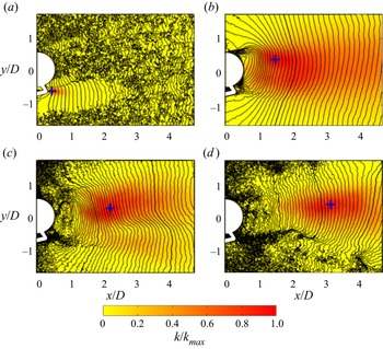The shedding modes and the harmonics obtained for $\theta =110^\circ$ are shown in figure 8 and are qualitatively similar to $\theta = 90^\circ$.

Figure 8.

Modes associated with (a) control rod shedding frequency and (b) cylinder shedding frequency at $\theta =110^\circ$. Panels (c,d) show the second and third harmonics of the main cylinder's shedding mode, respectively. The filled contour shows the energy of the modes while the contour lines represent isophase lines of transverse velocity fluctuation of the modes. The contour lines are shown from $-{\rm \pi}$ to ${\rm \pi}$ at step size (a) ${\rm \pi} /2$, (b) ${\rm \pi} /15$, (c) ${\rm \pi} /10$ and (d) ${\rm \pi} /7$. The (blue) + sign shows the location where the kinetic energies of the modes attain a maximum.

5.2. Secondary modes and phase averaging

Although the fundamental shedding modes of the control rod, the main cylinder and its harmonics were captured in the OMD spectrum, the secondary modes (as shown in figure 5c,e) were not captured by the OMD spectrum (see Appendix A). Similar observations were reported by Baj & Buxton (Reference Baj and Buxton2017) where OMD was incapable of identifying modes in and around the secondary frequencies even when the rank of the projection/dynamic matrices was set to very high values. However, since we have the phase reference of the secondary modes, i.e. $f_c\pm f_m$, we can use phase averaging (see for instance Reynolds & Hussain Reference Reynolds and Hussain1972; Cantwell & Coles Reference Cantwell and Coles1983) to extract the modes associated with the secondary frequencies. Essentially, we apply phase averaging separately for the two secondary modes with corresponding phase references. In order to obtain the phase averaged flow field at the reference frequencies $f_c\pm f_m$, we divide the snapshots into 16 phase bins with phases ranging from $-{\rm \pi}$ to ${\rm \pi}$. Subsequently, we take the second Fourier mode of the phase-averaged flow field in order to produce a complex spatial mode that mimics the OMD modes. Thereupon, the complex coefficients of the secondary modes are obtained in a similar fashion to the OMD modes. We encourage readers to refer to Baj & Buxton (Reference Baj and Buxton2017) for an extensive description of identification of the secondary modes using phase averaging.

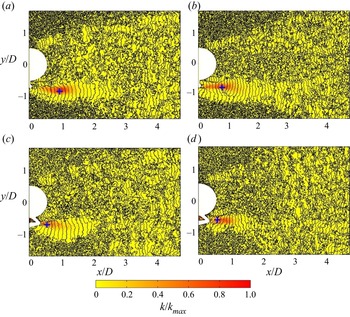
The secondary modes identified for $\theta = 90^\circ$ and $110^\circ$ are shown in figure 9. Note that both modes present a large phase-correlated region in the vicinity of the control rod, although they are not as prominent as the modes shown in figure 7 or figure 8. Similar to the control rod's shedding mode, a small phase-correlated region is observed towards the upper shear layer of the main cylinder for all the secondary modes. However, the energy content in this region is again negligible and hence not considered for further analysis. Note that the strength and the spatial extent of the modes depends on the control rod angle. Recall from figure 5(c,e), that the secondary modes were more prominent for $\theta =90^\circ$ compared with $\theta =110^\circ$. We observe the same story in figure 9. The energy content and the spatial extent of both modes diminishes for $\theta =110^\circ$ compared with $\theta =90^\circ$. Similarly to figure 7, the location of maximum kinetic energy of the secondary modes is also shown by a (blue) + sign. The location of peak kinetic energy, as well as the spatial orientation of the modes, reveals some interesting facts. Recall from figure 5(c,e) that the high-frequency secondary mode was located more towards the separated shear layer between the main cylinder and the control rod whereas the lower secondary frequency was more towards the lower shear layer. The orientation of the spatial region where most of the energy of the modes is concentrated in figure 9 reveals similar trends, i.e. most of the energy of the lower secondary mode is concentrated towards the lower shear layer of the control rod and vice versa. The kinetic energy of the secondary modes peaks farther downstream compared with the control rod's fundamental shedding mode for which the peak was located very close to the control rod. This difference in the location of peak kinetic energy was also noted by Baj & Buxton (Reference Baj and Buxton2017) and it hints at the fact that a different mechanism is involved behind the formation of the secondary modes. Interestingly, the kinetic energy of the secondary modes at $\theta =110^\circ$ peaks much earlier in comparison with $\theta =90^\circ$ and it correlates well with the closer wake intersection points observed for $\theta =110^\circ$ in figure 4(b). This correlation between the location of wake intersection points and kinetic energy maxima implies that the secondary modes ought to be related to the interaction between the main cylinder's and control rod's fundamental shedding modes. However, the locations of the kinetic energy maxima of the secondary modes do not exactly coincide with the corresponding wake intersection points and are slightly upstream of the corresponding wake intersection points identified in § 3 (see figure 4). For a deeper understanding of the formation of the modes we evaluate the kinetic energy budget for each of the modes in the next section.

Figure 9.

Energy and isophase lines associated with (a) low-frequency ($f_c-f_m$) and (b) high-frequency ($f_c+f_m$) secondary modes for $\theta =90^\circ$. The corresponding modes for $\theta =110^\circ$ are shown in (c,d). The contour lines are shown between $-{\rm \pi}$ to ${\rm \pi}$ at a step size of ${\rm \pi} /2$ for all the modes. The (blue) + sign shows the location where kinetic energy is maximum.

6. Energy budget equations

Turbulent kinetic energy (TKE) transport in free shear flows has been the subject of numerous studies (Panchapakesan & Lumley Reference Panchapakesan and Lumley1993; Liu & Thomas Reference Liu and Thomas2004; Morris et al. Reference Morris, Biswas, Aleyasin and Tachie2021) using a generic TKE transport equation (for instance see Hinze (Reference Hinze1975)). However, for a multiscale flow like the present problem, a separate TKE transport equation is required for the coherent motions present in the flow to track energy exchanges to/from the individual coherent motions (as well as the mean flow and stochastic fluctuations). Reynolds & Hussain (Reference Reynolds and Hussain1972) derived separate TKE transport equations for the mean, coherent and stochastic part of the flow. Here, the average kinetic energy per unit mass in the flow was represented as

(6.1)

\begin{equation} \frac{1}{2} \overline{u_i u_i} = \frac{1}{2}\bar{u}_i\bar{u}_i + \frac{1}{2}\overline{\tilde{u}_i\tilde{u}_i} + \frac{1}{2}\overline{u''_i u''_i}. \end{equation}

Along similar lines, Baj & Buxton (Reference Baj and Buxton2017) derived the kinetic energy budget equations identified using the multiscale triple decomposition technique discussed earlier. The average kinetic energy at a point is then described as

(6.2)

\begin{equation} \frac{1}{2} \overline{u_i u_i} = \frac{1}{2}\bar{u}_i\bar{u}_i + \frac{1}{2} \sum_l \overline{\tilde{u}^{f_l}_{i}\tilde{u}^{f_l}_{i}} + \frac{1}{2}\overline{u''_i u''_i}, \end{equation}

where $\tilde {u}^{f_k}_i$ is the $i$th velocity component of the coherent motion with characteristic frequency $f_k$. Baj & Buxton (Reference Baj and Buxton2017) showed that the correlations such as $\overline {\tilde {u}^{f_l}_{i} u''_i}$ and $\overline {\tilde {u}^{f_l}_{i} \tilde {u}^{f_m}_{i}}$ were negligible compared with the terms on the right-hand side of (6.2) (see Appendix D of Baj & Buxton (Reference Baj and Buxton2017)). The authors derived separate TKE transport equations for the mean and stochastic component of the flow as well as for each of the coherent motions present in the flow. However, we note that the spatial resolution of the current PIV measurements is insufficient to resolve the dissipation rate of TKE, which is a major contributor to the budget for the stochastic fluctuations, thereby precluding us from considering the stochastic energy budget. Nevertheless, as the main motivation of the present manuscript is to study the energy exchanges between the mean flow and the coherent motions, and also between different coherent motions, we restrict ourselves to the TKE transport equations for the mean component and the coherent motions. The TKE transport equation for the mean component and the coherent motions are shown symbolically in (6.3) and (6.4), respectively; readers are referred to Baj & Buxton (Reference Baj and Buxton2017) for the full derivation of these equations and the various terms contained therein,

(6.3)

\begin{gather} {-\bar{C} -\sum_l \tilde{P}_l - P^{''} - \bar{\epsilon} +\bar{D} = 0}, \end{gather}

(6.4)

\begin{gather} {\frac{\partial \tilde{k}_l}{\partial t} ={-}\tilde{C}_l + \tilde{P}_l - \widehat{P_l} +\tilde{T}^+_l - \tilde{T}^-_l - \widetilde{\epsilon_l} +\widetilde{D_l} }. \end{gather}

In (6.3), the term $-\bar {C}$ is the convection term and $-\sum _l \tilde {P}_l$ denotes the net coherent energy production term (from the mean flow) which is the sum of the energies transferred to the individual coherent motions from the mean flow (i.e. $\tilde {P}_l$ for the $l$th coherent motion). Here, $\tilde {P}_l$ is defined as $-\sum _{f_s} \overline {\tilde {u}^{f_s}_{i} \tilde {u}^{f_l}_{j} ({\partial \bar {u}_i}/{\partial x_j})}$, where $s$ can be any coherent motion including the $l$th coherent motion. The terms $P^{''}$, $\bar {\epsilon }$ and $\bar {D}$ represent the production of stochastic turbulent kinetic energy directly from the mean flow, direct dissipation from the mean flow and the mean diffusion terms, respectively.

Contrastingly to (6.3), in (6.4) $\tilde {P}_l$ appears with a positive sign, i.e. it acts as a source for the $l$th coherent motion. The term $\hat {P}_l$ is the production of stochastic turbulent kinetic energy term from the $l$th coherent motion and appears as a sink. Here $\tilde {\epsilon }_l$ and $\tilde {D}_l$ represent the dissipation of kinetic energy (by the $l$th coherent motion) and diffusion terms, respectively. Note that two new terms appear in the kinetic energy budget equation for coherent structures, $\tilde {T}^+_l$ and $\tilde {T}^-_l$, which are referred to as the triadic energy production terms. These terms account for the energy transfer between different coherent structures through nonlinear interactions. For instance, the term $\tilde {T}^+_l$ accounts for the energy gained by the $l$th coherent motion from other coherent modes and is defined as

(6.5)

\begin{equation} \tilde{T}^+_{l} ={-}\frac{1}{2}\sum_{f_s,f_t}\overline{u^{f_l}_i u^{f_t}_j \frac{\partial u^{f_s}_i}{\partial x_j}}. \end{equation}

Baj & Buxton (Reference Baj and Buxton2017) argued that this term could be non-negligible only when the coherent structures involved in the energy exchange process formed a triad, i.e. $f_l\pm f_s\pm f_t=0$. Similarly, $\tilde {T}^-_l$ represents the energy lost by the $l$th mode to other coherent motions and is defined as

(6.6)

\begin{equation} \tilde{T}^-_{l} ={-}\frac{1}{2}\sum_{f_s,f_t}\overline{u^{f_s}_i u^{f_t}_j \frac{\partial u^{f_l}_i}{\partial x_j}}. \end{equation}

Note that, in both $\tilde {T}^+_l$ and $\tilde {T}^-_l$, the $t$th mode acts merely as a catalyst and does not take part in the energy transfer process directly. Baj & Buxton (Reference Baj and Buxton2017) grouped these two terms together and represented them as a single triadic energy transfer term.

6.1. Mean energy budget

Let us first investigate the terms of the mean TKE budget equation (6.3) for the flow under investigation. As the flow is primarily two-dimensional, the contribution of the out-of-plane component of velocity can be expected to be small (Baj & Buxton Reference Baj and Buxton2017; Portela, Papadakis & Vassilicos Reference Portela, Papadakis and Vassilicos2017). We thus choose to ignore the terms containing the out-of-plane velocity component as well as out-of-plane velocity gradients for evaluating the TKE budget terms. These are expected to be small but will (in part) appear in the residual $\zeta$, alongside other inaccessible terms such as the pressure-diffusion term. The pressure-diffusion term has been neglected in several other works on free shear flows and its contribution has been estimated from a balance of the budget (for example see Browne, Antonia & Shah (Reference Browne, Antonia and Shah1987) for a self-similar wake and Panchapakesan & Lumley (Reference Panchapakesan and Lumley1993) for an axisymmetric jet). Baj & Buxton (Reference Baj and Buxton2017) ignored the pressure–velocity coupling while calculating the diffusion term and argued that the high residuals observed in the near field of their multiscale geometry was largely due to the neglected contribution of pressure.

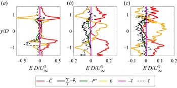
We present the different terms of (6.3) for $\theta =90^\circ$ in figure 10 at different streamwise stations. The energy terms are normalised by $U^3_{\infty }/D$. At $x/D=1$, the convection term ($-\bar {C}$) appears to be the dominant source term, while diffusion partly acts to counter it. The magnitude of the convection term is small but positive near the centreline of the main cylinder implying a slow spatial decay of kinetic energy in the vicinity of the centreline. This can be expected in the recirculation region as the magnitude of the streamwise velocity (which is negative) reduces as we approach the end of the recirculation region. The magnitude of the convection term, however, is large and positive outside the separated shear layers of the main cylinder implying a quick decay of the flow at this position. Note from figure 3(a) that at around $x/D=1$, the accelerated flow past the main cylinder quickly adjusts to the free stream value (i.e. a decay of mean kinetic energy) outside the separated shear layers, hence explaining the positive peaks observed in the convection term. Comparing the sink terms at this location, it can be discerned that a considerable amount of energy is transferred to the stochastic motion from the mean flow. However, farther downstream, at $x/D=2$ (see figure 10b), the major energy sink is the coherent energy production term. Note from figure 6 that at this location, the fundamental shedding mode of the main cylinder as well as its harmonics are significantly stronger compared with $x/D=1$. As a result, a higher coherent energy production at $x/D=2$ can be expected. The convection term is nearly zero at the centreline as the location is close to the edge of the recirculation region. The peaks of the convection terms are now milder and appear further apart from the centreline. At $x/D=3$, the terms show the same qualitative trends as for $x/D=2$, however, the convection term becomes positive near the centreline implying a spatial accumulation of kinetic energy or wake recovery. The ($\sum _l -\widetilde {P_l}$) term at this location is lower compared with $x/D=2$ implying a decrease in the strength of the coherent motions also observed in figure 6(a). Energy lost due to direct dissipation from the mean flow is negligible at all of the streamwise locations considered as expected.

Figure 10.

Terms of the mean kinetic energy budget for $\theta =90^\circ$ at (a) $x/D=1$, (b) $x/D=2$ and (c) $x/D=3$. The energy budget terms (denoted by $E$ in the figure) are non-dimensionalised by $U_{\infty }^3/D$.

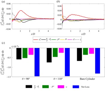
In order to obtain a clearer picture, we integrate the profiles of the different terms of (6.3) with respect to transverse distance $y$ and show their evolution with streamwise distance for $\theta =90^\circ$ and the bare cylinder in figure 11. The corresponding figure for $\theta =110^\circ$ is not shown, for brevity, due to its qualitative similarity with $\theta =90^\circ$. The limits of integration ($y1$ and $y2$) are taken to be $-1.65D$ and $1.65D$, respectively, which are slightly smaller than the limit of the field of view. The integrated terms remain apparently insensitive to slight variation in $y1$ and $y2$. Figure 11 shows that the convection term is dominant everywhere for both $\theta =90^\circ$ and the bare cylinder. The coherent energy production term is the main sink of energy for both cases, however, this term also shows two minima for $\theta =90^\circ$ (unlike the bare cylinder) due to the presence of two distinct wake-generating bodies. The minima in the coherent energy production term associated with the main cylinder's shedding mode is significantly reduced for $\theta =90^\circ$ compared with the bare cylinder, showing the effectiveness of the control rod in controlling the main cylinder's shedding mode. Apart from the primary shedding modes, the coherent energy production term includes a contribution from the harmonics of the main cylinder's shedding mode as well. Note that although we show the evolution of the $\sum - \tilde {P}_l$ term from close to the control rod surface, the second and third harmonics are largely incoherent before $x/D \approx 1.3$. As a result, the $\sum - \tilde {P}_l$ term can be expected to be slightly noisy close to the main cylinder–control rod assembly. Nevertheless, since the $\tilde {P}_l$ terms for the harmonics are an order of magnitude weaker than those of the primary shedding modes (as we will show in § 6), they do not affect the $\sum - \tilde {P}_l$ term significantly in this region. Apart from the $\sum - \tilde {P}_l$ term, some amount of energy is also lost through the stochastic energy production and dissipation terms, however, their relative contribution in both cases is hard to assess from figure 11.

Figure 11.

Streamwise evolution of the integrated kinetic energy budget terms for (a) $\theta =90^\circ$ and (b) bare cylinder. The horizontal (– $\cdot$ –) line shows the $0$ level for a reference. (c) Net contribution of different sink terms. The energy budget terms are denoted by the generic $E$ letter.

We thus further integrate the sink terms shown in figure 11(a,b) with respect to $x$ to obtain the net contribution of each of the terms across the whole field of view. The results are shown in figure 11(c) for $\theta =90^\circ$, $\theta =110^\circ$, and the bare cylinder. For $\theta =90^\circ$ and the bare cylinder, the domain of integration is taken from $x1 = 0.1D$, which is close to the control rod or the left limit of the field of view to $x2=4.5D$. Note from figure 11(c) that for all cases, the major energy loss is due to the coherent energy production term followed by stochastic energy production and direct dissipation. Interestingly, the net energy lost to the coherent motions for $\theta =90^\circ$ is the least among the three cases, followed by the bare cylinder and $\theta =110^\circ$. It indicates that the coherent motions on an aggregate are the most energetic for $\theta =110^\circ$ and least energetic for $\theta =90^\circ$. This observation correlates well with the finding of Cicolin et al. (Reference Cicolin, Buxton, Assi and Bearman2021) that the fluctuating loads acting on the main cylinder at $\theta =90^\circ$ were lower than the bare cylinder, while for $\theta =110^\circ$ they were higher. Further, the authors reported that the net drag acting on the combined assembly of the main cylinder and control rod was close for $\theta =90^\circ$ and $\theta =110^\circ$, while both were nearly $10\,\%$ larger than the drag on the bare cylinder. A remarkably similar trend is revealed by the blue bars representing the net losses in figure 11(c), i.e. the net losses suffered by the mean flow for both $\theta =90^\circ$ and $\theta =110^\circ$ are similar and both are $10\,\%$ larger than that of the bare cylinder. Note that drag must be thermodynamically linked to total dissipation and the pink columns represent the energy dissipated directly from the mean flow only. Considering the cascade of energy, the energy transferred to the coherent motions and stochastic motion from the mean flow is ultimately dissipated. Hence, figure 11(c) essentially shows that, although the total dissipation might be similar for both $\theta =90^\circ$ and $\theta =110^\circ$ (hence similar total drag), the path leading to total dissipation is different.

6.2. Energy budgets of primary shedding modes

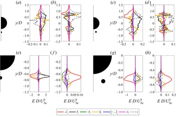
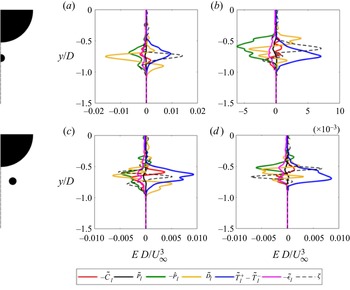
The terms of the coherent energy budget equations are first calculated for the main cylinder's ($f_m$) and control rod's shedding ($f_c$) modes and are shown in figure 12 for $\theta = 90^\circ$ and $110^\circ$. Figure 12(a) shows the energy budget terms in the near wake of the main cylinder at $x/D \approx 1.51$. Note from figure 6(a) that at this location the peak in the spectrum of the transverse velocity component attains its maximum value. At this location, the production term ($\tilde {P}_l$) is the main source of energy and is largely positive around the centreline. The convection term is largely negative in the vicinity of the shear layers of the main cylinder wake and acts as the major sink. It also shows that the energy of the mode is still building up and is yet to start decaying. Note that the $\tilde {P}_l$ and convection terms (which are the dominant source and sink terms, respectively) are asymmetric about the wake centreline ($y=0$) due to the presence of the control rod which alters the energy content in the lower shear layer of the main cylinder wake significantly, as observed in figure 7(b). Apart from the convection term, the other major contributor to the energy losses is the stochastic energy production term which is almost $30\,\%$ of the production term. The energy lost due to direct dissipation is not significant, neither is that due to the triadic energy production term.

Figure 12.

Coherent energy budget terms of the main cylinder's shedding mode at (a) the location where the spectral peak in the spectrum of transverse velocity component of the mode attains a maximum, i.e. $x/D \approx 1.51$ (b) wake intersection point ($x/D\approx 0.97$) for $\theta =90^\circ$. The same plots for $\theta =110^\circ$ are shown in (c) at $x/D \approx 1.48$ and (d) at $x/D \approx 0.76$, respectively. The corresponding budget terms for the control rod's fundamental shedding mode for $\theta =90^\circ$ are shown in (e) for $x/D \approx 0.1$ and in (f) for $x/D \approx 0.97$. The same plots for $\theta =110^\circ$ are shown in (g) at $x/D \approx 0.3$ and (h) at $x/D \approx 0.76$, respectively.

Figure 12(b) shows the energy budget terms for $f_m$ at the wake intersection point ($x/D \approx 0.97$) which is upstream of figure 12(a). The difference between the two stations is most pronounced in the $\tilde {P}_l$ term. The magnitude of the production term is much lower and it is positive only in the separated shear layers of the wake as the formation of the von Kármán vortex street behind the main cylinder is not complete at $x/D \approx 0.97$. Similarly, figure 12(c,d) show the kinetic energy budget terms for the main cylinder wake at the point of maximum transverse velocity ($x/D \approx 1.48$) and the wake intersection point ($x/D \approx 0.76$) at $\theta =110^\circ$. Note that the qualitative nature of the terms are very similar to $\theta =90^\circ$ although slight differences are seen in the magnitude of the terms. In particular, note that the $\tilde {P}_l$ term is almost twice larger for $\theta =110^\circ$ compared with $\theta =90^\circ$, which correlates well with the twice larger spectral peak for the transverse velocity at $f_m$ for $\theta =110^\circ$ observed in figure 6(b).

Figure 12(e) shows the kinetic energy budget terms for the control rod's fundamental shedding mode for $\theta =90^\circ$ at $x/D = 0.1$. This location is close to the point where the mode is the most energetic. At this location, we find that the mode is primarily energised by the mean flow through the $\tilde {P}_l$ term, whilst energy is mainly lost through convection and direct dissipation. All other terms are relatively small at this station. At the wake intersection point (figure 12f), however, the convection term is positive showing that the mode is now spatially decaying. This observation correlates well with the fast decaying transverse velocity amplitude of the control rod's shedding mode in figure 6(a). The production term is negligible and a significant amount of energy is drained by the stochastic energy production and dissipation terms at this location. Interestingly, at the wake intersection point, the triadic energy production term is non-negligible and acts as a sink for the control rod's shedding mode. The qualitative trends of the kinetic energy budget terms for $f_c$ remain very similar for $\theta =110^\circ$ (see figure 12g,h) apart from slight variation in the magnitudes. Figure 12(g) is shown at $x/D=0.3$, i.e. close to the point where $f_c$ is most energetic for $\theta =110^\circ$. Notably, the coherent energy production term ($\tilde {P}_l$) is weaker compared with that found in figure 12(e). The magnitude of the convection term at this location is also small indicating a relatively slow build up of energy. However, the magnitude of the convection term is higher compared with $\theta =90^\circ$ at the wake intersection point (figure 12h) indicating faster decay of the mode. All these points together agree well with the shorter extent of the control rod's wake seen in figure 4(b) for $\theta =110^\circ$.

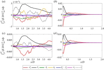
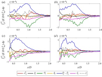
A clearer picture of the dynamics of each of the modes can be revealed by tracking the contribution of the terms with spatial distance in a continuous fashion. We therefore integrate the different terms in the kinetic energy budget equation of the coherent motions with respect to $y$ and show their evolution with streamwise distance in figure 13. Note that the dynamics of the modes at both values of $\theta$ is primarily governed by the $\tilde {P}_l$ and convection terms. The convection term shows a sign change for all the modes, implying an energy buildup and subsequent decay of the modes, although the rate of growth/decay is different for the modes and it also varies with $\theta$. For the main cylinder's shedding mode at $\theta =90^\circ$ (figure 13a), the main source of energy for the mode is the $\tilde {P}_l$ term everywhere in the domain, while the convection term and the $-\hat {P}_l$ term combined nearly balances the net gain due to it. The evolution of the $\tilde {P}_l$ term looks quite similar to the evolution of the mode's spectral peak in figure 6(a) and it peaks around $x/D=1.5$ which is where the amplitude of transverse velocity of the mode is also maximum. Although figure 13(c) for $\theta =110^\circ$ shows a qualitatively similar trend to figure 13(a), note that the production term then drops off much earlier. The convection term also becomes positive much earlier, implying that the mode starts to decay much earlier in comparison with $\theta =90^\circ$. This result correlates well with the shorter recirculation region observed for $\theta =110^\circ$ in figure 3(b) compared with $\theta =90^\circ$. Further, note that the peak of the production term at $\theta =110^\circ$ is almost twice that compared with $\theta =90^\circ$ which explains the twice higher spectral peak observed for $f_m$ at $\theta =110^\circ$ in figure 6(b). Similarly we show the streamwise evolution of the kinetic energy budget terms for the control rod's fundamental shedding mode at $\theta =90^\circ$ and $\theta =110^\circ$ in figures 13(b) and 13(d), respectively. The trends look very similar to each other apart from slight differences in the amplitudes. The production term falls off sharply within a short streamwise distance and correlates well with the short streamwise extent of the modes seen in figures 6 and 7(a). The convection term is roughly negatively correlated with the production term as also observed for the main cylinder's shedding mode $f_m$ and is the main sink of energy. The contribution from all the other terms as a whole is relatively small compared with the convection and $\tilde {P}_l$ term.

Figure 13.

Streamwise evolution of the kinetic energy budget terms for (a) the main cylinder's and (b) the control rod's fundamental shedding modes at $\theta =90^\circ$. Panels (c,d) show the same $\theta =110^\circ$. The horizontal (– $\cdot$ –) line shows the $0$ level for a reference.

We now cast a closer look at the nonlinear triadic interaction term and also compare it with the $\tilde {P}_l$ term. Note that the evolution of the triadic interaction term shown in figure 13 is the sum of contributions from all other modes forming a triad with that respective mode. For instance, for a triad containing $f_p$, $f_q$ and $f_r$, the net triadic energy transfer to mode $f_p$ (denoted by $\tilde {T}^+_{p} - \tilde {T}^-_{p}$) is essentially the sum of two non-negligible transfers as follows:

(6.7)

\begin{equation} \tilde{T}^+_{p} - \tilde{T}^-_{p} = \frac{1}{2}\left(- \overline{u^{f_{p}}_i u^{f_q}_j \frac{\partial u^{f_r}_i}{\partial x_j}} +\overline{u^{f_r}_i u^{f_q}_j \frac{\partial u^{f_{p}}_i}{\partial x_j}} \right) +\frac{1}{2}\left( -\overline{u^{f_{p}}_i u^{f_r}_j \frac{\partial u^{f_q}_i}{\partial x_j}} +\overline{u^{f_q}_i u^{f_r}_j \frac{\partial u^{f_{p}}_i}{\partial x_j}} \right). \end{equation}

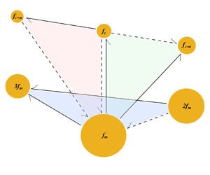
Here, the first term on the right-hand side accounts for the net energy exchange between $f_p$ and $f_r$, while the second term captures the same between $f_p$ and $f_q$. We now try to understand the overall contributions of each of these individual energy transfers between two modes integrated over the entire domain of interest. Note that the main cylinder's shedding mode forms three triads with the other modes, which are $[f_m, f_c, f_{c-m}]$, $[f_m, f_c, f_{c+m}]$ and $[f_m, 2f_m, 3f_{m}]$. Hence, we can expect nonlinear energy transfer between $f_m$ and all the other modes. The control rod's shedding mode ($f_c$) can interact only with $f_m$ and the secondary modes, however. While integrating these nonlinear energy transfers as well as the $\tilde {P}_l$ term of the modes over the entire domain, care must be taken for the selection of the left limit of the domain ($x1$) for each of the terms. For instance, for the $\tilde {P}_l$ term of the main cylinder's shedding mode, $x1$ must be set to $0.5D$ in order to avoid the spatially incoherent region of the mode adjacent to the cylinder. For the control rod's shedding mode, however, $x1$ must be set close to the control rod (i.e. $<0.5D$) to capture the contribution of the $\tilde {P}_l$ term (see figure 13b). Hence, for the control rod's shedding mode as well as the secondary modes at $\theta =90^\circ$, $x1$ is set to be $0.1D$. Similarly, for $\theta =110^\circ$ the corresponding $x1$ is chosen to be $0.3D$ which is sufficiently close to the control rod. The harmonics of the main cylinder's shedding mode are energetic farther downstream and shows a large spatially incoherent region at $x/D \lesssim 1.3$. Therefore, for the harmonics at $\theta =90^\circ$, $x1$ is chosen to be $1.3D$. A sensitivity analysis is performed by varying $x1$ around $1.3D$ and obtaining the integrated energy terms for the harmonics which is included in Appendix C. It is found that lowering $x1$ below $1.3D$ does not introduce appreciable changes to the energy terms of interest.

In figure 14, the two thick bars on the left show the net contribution from $\tilde {P}_l$ and the triadic interaction term ($\tilde {T}_l$), respectively, to the $l$th mode, whilst the thinner bars towards the right break down the contributions from different modes to the overall triadic interaction term. All energy terms are obtained by performing integration over the domain spanned by $[(x1,y1), (x2,y2)]$, with $x1$ varying depending on the particular mode as discussed previously and $x2,y1$ and $y2$ set close to the edge of the domain avoiding spurious vectors towards the boundary. In figure 14, a positive contribution (i.e. energy is gained by the mode) is shown with a black bar whilst red bars signify a loss of energy. For the main cylinder's fundamental shedding mode (figure 14a) the net triadic production is positive, though negligible in comparison with production from the mean flow. The main source of triadic energy gain of $f_m$ is the second harmonic ($2f_{m}$), while the energy transfers with the other modes is an order of magnitude smaller. This energy transfer between the main cylinder's fundamental shedding mode and its harmonics differs significantly from the findings of Jin et al. (Reference Jin, Symon and Illingworth2021). However, the authors reported the energy transfers between the modes at a Reynolds number two orders of magnitude lower than the present study and hence a significant difference can be expected in the energy transfer processes.

Figure 14.

Net energy transfers through coherent energy production and nonlinear triadic energy transfer terms for (a) the main cylinder's fundamental shedding mode and (b) the control rod's fundamental shedding mode for $\theta =90^\circ$. Black bars show a gain of energy and red bars show a loss of energy for the respective mode.

Finally, it is also interesting to note that the two secondary modes behave in an opposite fashion to one another, i.e. the low-frequency mode ($f_{c-m}$) gains some energy from $f_m$ whilst the high-frequency mode ($f_{c+m}$) transfers almost the same amount of energy to $f_m$. Unlike the main cylinder's fundamental shedding mode, the control rod's shedding mode ($f_c$) is solely energised by the mean flow. This mode gives away an almost equal amount of energy to both the secondary coherent structures.

6.3. On the origin of the secondary coherent structures

Let us now perform the same analysis and obtain the terms of the kinetic energy budget equations for the secondary coherent motions shown in figure 9. Figure 15 shows the energy budget terms for the secondary modes at the wake intersection points for $\theta = 90^\circ$ and $110^\circ$. Note that the qualitative trend for the modes is remarkably similar for both values of $\theta$, although subtle differences do exist. Unlike the primary shedding modes discussed earlier, the main source of energy for the secondary modes is the triadic energy production term whereas the energy production from the mean flow is negligible, and even slightly negative; similar to the findings of Baj & Buxton (Reference Baj and Buxton2017). This fundamental difference in the primary energy source of the mode justifies naming them as ‘secondary’ since they are not directly energised by the mean flow. Note that the secondary modes play a major role in the energy cascade as a significant amount of energy is drained into stochastic turbulent motion through them. The net contribution of the diffusion and convection terms at this station for both the modes is small and is rather inconclusive.

Figure 15.

Kinetic energy budget terms for (a) low- and (b) high-frequency secondary coherent modes for $\theta =90^\circ$ at the wake intersection point. Panels (c,d) show the same for $\theta =110^\circ$ at the corresponding wake intersection point.

A clearer picture is obtained as we observe the streamwise evolution of the various integrated kinetic energy budget terms in figure 16. For both the low-frequency and high-frequency secondary modes, the major source of energy is the triadic production term everywhere in the domain whereas production from the mean flow is negligible. Further, note that the triadic production term of the secondary modes at $\theta =90^\circ$ peaks farther downstream than for $\theta =110^\circ$. Recall from figure 9 that the maximum of the kinetic energy of the secondary modes indeed appeared slightly downstream for $\theta =90^\circ$ compared with $\theta =110^\circ$, and the evolution of the triadic energy production term explains this observation. This is also in line with the nearer wake intersection point observed for $\theta =110^\circ$ compared with $\theta =90^\circ$. Baj & Buxton (Reference Baj and Buxton2017) found that the low-frequency secondary mode was more spatially persistent compared with the high-frequency one. We observe something quite similar for our configuration. Note that at $\theta =90^\circ$, the convection term becomes positive earlier for the high-frequency secondary mode, implying that the high-frequency secondary mode starts to decay earlier compared with its low-frequency counterpart. A similar trend, although not pronounced, is observed for $\theta =110^\circ$ as well. Moreover, see that for both values of $\theta$, the triadic energy production term drops off earlier for the high-frequency secondary mode. It is believed that a combination of both of these effects results in a more spatially persistent low-frequency secondary mode compared with the high-frequency one.

Figure 16.

Streamwise evolution of the integrated kinetic energy budget terms for (a) low- and (b) high-frequency secondary modes for $\theta =90^\circ$. Panels (c,d) show the same for $\theta =110^\circ$.

Let us now compare the relative contributions of the nonlinear energy transfers between two modes in the triads $[f_m, f_c, f_{c \pm m}]$. The spatial evolution of the nonlinear energy transfer terms for $\theta =90^\circ$ are shown in figure 17(a,b) for the low-frequency and high-frequency secondary modes, respectively. The solid black curve shows the nonlinear energy transfer from $f_c$ to $f_{c\pm m}$, $\tilde {T}_{f_c \rightarrow f_{c\pm m}}$ defined as

(6.8)

\begin{equation} \tilde{T}_{f_c \rightarrow f_{c\pm m}} ={-}\frac{1}{2}\overline{u^{f_{c\pm m}}_i u^{f_m}_j \frac{\partial u^{f_c}_i}{\partial x_j}} +\frac{1}{2}\overline{u^{f_c}_i u^{f_m}_j \frac{\partial u^{f_{c\pm m}}_i}{\partial x_j}}. \end{equation}

Here the main cylinder's shedding mode ($f_m$) acts as the catalyst. The net nonlinear energy gain for both the secondary modes almost entirely comes from the control rod's shedding mode ($f_c$). The dashed vertical line shows the location of the wake intersection point. In the vicinity of the wake intersection point, the low-frequency secondary mode ($f_{c-m}$) receives a small amount of energy from $f_m$, while the high-frequency secondary mode ($f_{c+m}$) loses some energy to $f_m$. Further, $f_m$ receives some energy from $f_c$ in the presence of $f_{c-m}$, whilst the direction of the energy transfer gets reversed in the presence of $f_{c+m}$. The exact same sequence of energy transfers was reported by Baj & Buxton (Reference Baj and Buxton2017) near the wake intersection points in the wake of a multiscale array of rectangular prisms.

Figure 17.

Streamwise evolution of certain triadic energy transfer terms for (a) low- and (b) high-frequency secondary modes at $\theta =90^\circ$.

Similar to figure 14 we integrate the production terms and the triadic energy transfer terms from other modes over the whole domain for the secondary modes, starting from $x/D=0.1$. The results are shown in figure 18. As expected the main source of energy for both the secondary modes is the nonlinear energy transfer from $f_c$ and production from the mean flow is negligible. The net energy transfer between $f_m$ and the secondary modes is almost equal in magnitude and opposite in direction. Hence, we find that the sequence of energy transfers first reported by Baj & Buxton (Reference Baj and Buxton2017) not only applies locally near the wake intersection points, but also applies globally when the net energy transfer in the domain is considered. Indeed, such similarity in the energy transfer process observed in two different flows is remarkable and it further strengthens the notion that this pattern of energy exchange in a triad of primary and secondary coherent motions is universal in multiscale flows. Note that the flow we consider in the present manuscript is different from the flow investigated by Baj & Buxton (Reference Baj and Buxton2017) in two major aspects. (1) For the present case the spectral separation of the two primary modes is much larger (see figure 5c,e). (2) The sizes of the control rod and the cylinder differ by an order of magnitude in the present case hence the energy difference between the two primary coherent modes is quite large compared with Baj & Buxton (Reference Baj and Buxton2017). The fact that we still find similar energy exchanges in two fundamentally different flows is both fascinating and significant for further understanding multiscale flows.

Figure 18.

Net energy transfer through coherent energy production and nonlinear triadic energy transfer terms for (a) low- and (b) high-frequency secondary modes at $\theta =90^\circ$. The colours of the bars bear the same meaning as in figure 12.

6.4. Energy exchanges for the harmonics

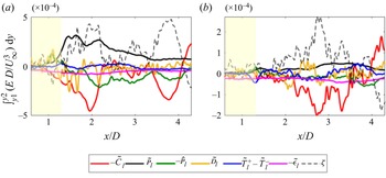
Let us apply the same analysis for the harmonics of the main cylinder's shedding mode ($f_m$) to better understand the nature of the modes. The evolution of the integrated TKE budget terms are shown in figure 19 for $\theta =90^\circ$. Due to the qualitative similarity of the modes for $\theta =90^\circ$ and $\theta =110^\circ$, we restrict the analysis only to $\theta =90^\circ$. As we discussed earlier, the second and third harmonics of the main cylinder's shedding mode being spatially coherent beyond $x/D \approx 1.3$, we exclude the region highlighted with a yellow colour in figure 19 for further analysis. At first glance the terms in figure 19 look much noisier compared with the corresponding ones for the primary modes ($f_c$, $f_m$) and even the secondary modes ($f_c \pm f_m$) seen earlier. Nevertheless, several insightful conclusions can be drawn from the plots. First of all, note that unlike the secondary modes observed in figure 16, the main source of energy for both the harmonics is still production from the mean flow. This is in contrast to the observation of Jin et al. (Reference Jin, Symon and Illingworth2021) who found that the primary source of energy for the harmonics was the fundamental shedding mode at a $Re = 100$. This fundamental difference in the primary energy source of the harmonics is believed to be a manifestation of the larger $Re$ in the present case. However, the contribution of the nonlinear triadic interaction term is not negligible as observed for the primary modes in figure 13. Therefore, the harmonics can neither be termed as ‘primary’ modes which feed from the mean flow nor ‘secondary modes’ which derive their energy from the primary modes alone. The harmonics rather behave as ‘intermediate’ or ‘mixed’ modes at our $Re$. The modes drain a significant amount of energy to stochastic turbulent kinetic energy and dissipation as can be seen from figure 19. The trends of the convection and diffusion terms, however, are comparatively noisy and hard to draw conclusions from. Figure 20 shows the total contribution from the production term and triadic interaction terms for the harmonics. Note that the magnitude of the triadic energy transfer term is smaller compared with the production term as expected. However, the triadic interaction term can still be significantly important and, in fact, it is a significant source of energy for the third harmonic. The third harmonic is positively energised by both the fundamental mode and the second harmonic, while the nonlinear energy gain of the fundamental mode is mainly due to the second harmonic.

Figure 19.

Streamwise evolution of the kinetic energy budget terms for (a) the second harmonic ($2f_m$) and (b) the third harmonic ($3f_m$) of the main cylinder shedding mode for $\theta =90^\circ$. The region highlighted in yellow colour is excluded in further analysis to avoid spatially incoherent region of the modes.

Figure 20.

Net contribution from the production and triadic interaction terms for (a) the second harmonic ($2f_m$) and (b) the third harmonic ($3f_m$) of the main cylinder. The colours of the bars bear the same meaning as in figure 12.

7. Summarising the energy cascade

We sum up the entire energy transfer process from the mean flow to the coherent motions, and also between the different coherent motions through a flow diagram shown in figure 21. The six modes identified in the flow, namely $f_m, 2f_m, 3f_m, f_{c-m}, f_c, f_{c+m}$, are shown as yellow circles. For visual representation, the modes are placed from bottom to top in increasing order of frequency, although not to scale. Further, the lower frequencies are shown as a larger circle as a representation of their larger spatial extent. The full headed arrows show the net energy transfer between the mean flow and the coherent motions. The full headed black arrows show energy gain of the modes, whilst red arrows show loss of energy. The half-headed arrows on the other hand represent nonlinear energy transfer between two modes. Solid arrows represent energy transfer from low frequency to high frequency whilst dashed arrows represent energy transfer from high frequency to low frequency, or an inverse energy cascade. Note that the primary modes, $f_m$ and $f_c$, draw the largest amount of energy from the mean flow, whilst the energy transfer to the secondary modes ($f_{c\pm m}$) from the mean flow is negligible and negative in the domain of investigation similar to the findings of Baj & Buxton (Reference Baj and Buxton2017). The primary energy source of the harmonics is also the mean flow, however, the energy received by the harmonics is significantly lower compared with the primary modes. The three triads (each triad consisting of three different frequencies whose linear combination sum to zero) formed by the half-headed arrows can be identified as the regions shaded with different colours. In triad 1 and triad 2 (shaded by pink and green colours, respectively), $f_c$ shares almost the same amount of energy to $f_{c+m}$ and $f_{c-m}$. During both of these transfers, $f_m$ acts as the mediator. In triad 1, $f_{c+m}$ then transfers some of its energy to $f_m$. Interestingly, $f_m$ then transfers almost the same amount of energy to $f_{c-m}$. As a consequence, the net nonlinear energy gain of the low-frequency secondary mode is higher than the high-frequency secondary mode and this is consistent with the greater spatial persistence of the lower secondary mode observed in our current work and by Baj & Buxton (Reference Baj and Buxton2017). The energy transfers between $f_c$ and $f_m$ in the two triads are of similar magnitude and opposite in sign. These energy transfer trends in triad 1 and triad 2 are qualitatively identical to the findings of Baj & Buxton (Reference Baj and Buxton2017).

Figure 21.

Combined schematic energy transfer diagram for the different modes identified within the flow. The modes are arranged such that characteristic frequency of the modes increases from bottom to top. The thick full headed arrows show the net energy transfer between the various modes and the mean flow. The single headed arrows show the nonlinear triadic energy transfer between two modes. A solid line shows nonlinear energy transfer from low frequency to high frequency, whilst the dashed lines show energy transfers from high frequency to low frequency – an inverse cascade.

The third triad formed by the main cylinder's fundamental shedding mode and its harmonics is shown in a blue colour. Here $2f_m$ shares just around $8\,\%$ of the total energy it receives from the mean flow to $f_m$, nearly $34\,\%$ of which $f_m$ shares to $f_{3m}$. Note that almost half the nonlinear energy transfer for the present flow takes place from a high-frequency mode to a low-frequency mode, implying a significant amount of inverse energy cascade. Such inverse energy cascades have also been observed in the near wake of a multiscale (Gomes-Fernandes, Ganapathisubramani & Vassilicos Reference Gomes-Fernandes, Ganapathisubramani and Vassilicos2015; Baj & Buxton Reference Baj and Buxton2017) or single scale geometry (Jin et al. Reference Jin, Symon and Illingworth2021) and are important in understanding the interscale dynamics in flows consisting of several length/time scales.

8. Conclusion

Previous work by Cicolin et al. (Reference Cicolin, Buxton, Assi and Bearman2021) identified a number of coherent motions present in the flow past a cylinder with leeward control rod which are studied in greater detail in the present work. Aside from the frequencies associated with the fundamental shedding modes of the control rod and the main cylinder (and its harmonics), new secondary frequencies are observed in the spectra of the transverse velocity component that correspond to the sum and difference of the control rod's and main cylinder's fundamental shedding frequencies. The spatial configuration of these secondary frequencies observed at two different control rod angles reveals a remarkable similarity to the findings of Baj & Buxton (Reference Baj and Buxton2017) in the near wake of a multiscale array of rectangular prisms, hinting at a possible universality of the flow physics that generate these secondary modes. Specifically, the high-frequency secondary mode is found to position itself near the separated shear layer between the two wake-generating bodies, whilst the low-frequency secondary mode resides towards the opposite shear layer separating from the control rod. The multiscale triple decomposition method proposed by Baj et al. (Reference Baj, Bruce and Buxton2015) is applied to identify all of the coherent modes associated with each of the distinct frequencies identified within the flow. The secondary modes show a pronounced region of phase-correlated velocity (vorticity) that correlates well with the definition of a coherent structure proposed by Hussain (Reference Hussain1986).

For the first time we examine the energy exchanges taking place between the mean flow and the coherent motions in this particular flow, as well as the energy exchanges taking place between the various coherent motions in the context of the multiscale triple-decomposed energy budgets. The increase in the net energy losses suffered by the mean flow in the presence of the control rod compared with a bare cylinder (a cylinder without a control rod) is found to correlate remarkably well to the overall increase of mean drag for the main cylinder–control rod assembly reported by Cicolin et al. (Reference Cicolin, Buxton, Assi and Bearman2021) for the same control rod positions. Further, the net energy lost to the coherent motions ($\sum _l \widetilde {P_l}$) in the presence of the control rod agrees well with the relative changes in the fluctuating loads when compared with the bare cylinder, as reported by Cicolin et al. (Reference Cicolin, Buxton, Assi and Bearman2021).

Assessing the kinetic energy budgets of the individual coherent motions, we find that the fundamental shedding modes of the control rod and the main cylinder are energised by the mean flow. Contrastingly, the secondary coherent modes are found to be primarily energised by the nonlinear triadic energy transfer from the control rod's fundamental shedding mode. Although both secondary modes receive a nearly equal amount of energy from the control rod's fundamental shedding mode, the high-frequency secondary mode transfers some amount of energy to the main cylinder's fundamental shedding mode. This energy is subsequently transferred to the low-frequency secondary mode thereby forming a net inverse cascade. This sequence of energy transfers results in a more spatially persistent low-frequency secondary coherent mode compared with its high-frequency counterpart, a similar result to Baj & Buxton (Reference Baj and Buxton2017) for a different multiscale flow. The similarity between the secondary modes and their formation mechanisms, reported in two different studies consisting of markedly different wake-generating bodies further strengthens the notion of universality of these structures, and the nature of the energy transfers that feed them, in a general multiscale flow. Note that Baj & Buxton (Reference Baj and Buxton2017) tracked the energy exchanges for the secondary modes at selected spatial locations only. We reported the detailed spatial evolution of the nonlinear energy fluxes involving the secondary modes for the first time. It is found that the nonlinear energy flux from the control rod's shedding mode to the secondary modes, which is the main driver for the secondary modes, peaks in the vicinity of the wake intersection points, hence firmly establishing the importance of the wake intersection points in multiscale flows also identified by previous works (Mazellier & Vassilicos Reference Mazellier and Vassilicos2010; Gomes-Fernandes et al. Reference Gomes-Fernandes, Ganapathisubramani and Vassilicos2012; Baj & Buxton Reference Baj and Buxton2017). Integrating the nonlinear energy fluxes over the entire domain, we further report that the sequence of energy transfers between the primary and the secondary modes first reported by Baj & Buxton (Reference Baj and Buxton2017) not only applies locally at the wake intersection points, but also it applies for the net nonlinear energy transfers in the entire domain in which the secondary coherent structures are energetic. Interestingly, unlike the primary modes (the main cylinder's and control rod's shedding modes) and the secondary modes, it is shown that harmonics can be energised by both the mean flow and nonlinear triadic energy exchanges at our $Re$, implying a mixed or intermediate character of the modes at this $Re$.

Another facet of our work is that we find a significant amount of nonlinear energy transfer from high-frequency modes to low-frequency modes, a phenomenon commonly referred to as an inverse energy cascade in turbulent flows (Biferale, Musacchio & Toschi Reference Biferale, Musacchio and Toschi2012; Gomes-Fernandes et al. Reference Gomes-Fernandes, Ganapathisubramani and Vassilicos2015; Jin et al. Reference Jin, Symon and Illingworth2021). The recent study by Jin et al. (Reference Jin, Symon and Illingworth2021) showed that resolvent analysis (which is only based on the mean flow) failed to correctly capture the nonlinear energy transfers in a cylinder wake. Accordingly, the present analysis not only improves our understanding of the complex energy exchanges taking place in a widely studied flow, but it also offers an opportunity to better model the nonlinear energy transfers in flows of practical relevance.

Funding

N.B. acknowledges funding through the President's PhD Scholarship scheme at Imperial College London.

Declaration of interests

The authors report no conflict of interest.

Appendix A. The OMD spectrum

The OMD spectra for $\theta =90^\circ$ and $\theta =110^\circ$ is shown in figure 22. The least damped modes that correspond to the control rod's, and the main cylinder's, fundamental shedding modes and also the harmonics of the main cylinder's shedding mode are highlighted in the plot. Note that the frequencies of the modes remain more or less the same for both values of $\theta$ considered.

Figure 22.

The OMD spectra for $\theta =90^{\circ }$ and $\theta =110^{\circ }$.

Appendix B. Spatial resolution of the experimental data

We must verify if the spatial resolution of the current experimental data is enough to resolve the coherent structures produced from the control rod. The size of the interrogation windows in the current experiments is $0.37d$. However, the interrogation windows have a $75\,\%$ overlap along the $x$ and $y$ directions. As a result, the separation between adjacent vectors in the processed data is $\approx 0.09d$. Hence, even very close to the control rod, where the coherent structures can be assumed to be smallest, i.e. $\sim O(d)$, there are nearly 11 data points to capture their effect. Nevertheless, in order to verify if the current spatial resolution correctly captures the energy content in the control rod's wake, we compare results from two different data sets with different spatial resolutions. Apart from the data utilised in the present manuscript, Cicolin et al. (Reference Cicolin, Buxton, Assi and Bearman2021) also obtained data in a narrow strip spanning $\approx 0.41D$–$0.90D$ in the streamwise direction. The spatial resolution of the strip was $\approx 0.15d$ for each vector, and with a $75\,\%$ overlap it yields a distance of $0.03d$ between adjacent vectors. This additional data has a higher resolution than the data used in the current manuscript. For comparison, in a square of dimension $d \times d$ it has over 400 vectors whereas the manuscript's data has approximately 100. Figure 23(a) shows the evolution of mean kinetic energy in the vicinity of the control rod's wake at the midsection of the strip (camera 2), i.e. $x/D = 0.65$ for $\theta =90^\circ$. Camera 1 here refers to the data utilised in the present manuscript. The results from the two data sets agree remarkably well. We also perform the multiscale triple decomposition for the strip to extract the energy content in the control rod's shedding mode (denoted by $k_c$ here). Figure 23(b) here shows the profile of $k_c$ at the same streamwise location as figure 23(a) and the agreement between the two data sets is again satisfactory. Hence, we believe that the spatial resolution of the data set used in the present manuscript is sufficient to resolve the coherent structures produced from the control rod.

Figure 23.

(a) Mean kinetic energy and (b) kinetic energy of the control rod's shedding mode obtained from two data sets at $x/D = 0.65$.

Appendix C. Domain of integration for the energy terms of the harmonics

In order to understand the effect of the selected domain of integration on the net contribution from coherent energy production and triadic interaction terms for the harmonics of the main cylinder (as shown in figure 20), we vary the starting point of the domain of integration ($x1$) and show the variation in coherent energy production and triadic interaction term integrated over the entire domain in figure 24. It is found that for both the second and third harmonics, the net coherent energy production does not alter significantly if $x1$ is reduced below $1.3D$. Hence, for both the harmonics $x1$ is set to be $1.3D$.

Figure 24.

Effect of changing the domain of integration on the coherent energy production and triadic interaction terms of the (a) second and (b) third harmonics of the main cylinder's shedding frequency for $\theta = 90^\circ$.

Appendix D. Time series and FFT

Sample time series data of transverse velocity and corresponding FFT at sample spatial points are shown in figure 25. The time series in figure 25(a) is obtained at $x/D = 1, y/D = -0.7$, which is close to the control rod's wake. The corresponding FFT in figure 25(b) shows $f_m$, $f_c$ and $f_c\pm f_m$. Figure 25(c) show the time series at $x/D = 3, y/D = 0.35$, i.e. far from the control rod. The corresponding FFT in figure 25(d) shows $f_m$ and its harmonics.

Figure 25.

(a) Transverse velocity time series and (b) corresponding FFT spectra at $x/D = 1, y/D = -0.7$ showing the primary and secondary modes for $\theta = 90^\circ$. (c) Transverse velocity time series and (d) corresponding FFT spectra at $x/D = 3.5, y/D = 0.35$ showing the main cylinder's shedding mode and the harmonics at the same $\theta$.

References

REFERENCES

Alam, M.M., Moriya, M. & Sakamoto, H. 2003 Aerodynamic characteristics of two side-by-side circular cylinders and application of wavelet analysis on the switching phenomenon. J. Fluids Struct. 18 (3–4), 325–346.CrossRef Google Scholar

Baj, P., Bruce, P.J. & Buxton, O.R. 2015 The triple decomposition of a fluctuating velocity field in a multiscale flow. Phys. Fluids 27 (7), 075104.CrossRef Google Scholar

Baj, P. & Buxton, O.R. 2017 Interscale energy transfer in the merger of wakes of a multiscale array of rectangular cylinders. Phys. Rev. Fluids 2 (11), 114607.CrossRef Google Scholar

Baj, P. & Buxton, O.R. 2019 Passive scalar dispersion in the near wake of a multi-scale array of rectangular cylinders. J. Fluid Mech. 864, 181–220.CrossRef Google Scholar

Bearman, P. & Wadcock, A. 1973 The interaction between a pair of circular cylinders normal to a stream. J. Fluid Mech. 61 (3), 499–511.CrossRef Google Scholar

Berkooz, G., Holmes, P. & Lumley, J.L. 1993 The proper orthogonal decomposition in the analysis of turbulent flows. Annu. Rev. Fluid Mech. 25 (1), 539–575.CrossRef Google Scholar

Biferale, L., Musacchio, S. & Toschi, F. 2012 Inverse energy cascade in three-dimensional isotropic turbulence. Phys. Rev. Lett. 108 (16), 164501.CrossRef Google Scholar PubMed

Bingham, C., Morton, C. & Martinuzzi, R.J. 2018 Influence of control cylinder placement on vortex shedding from a circular cylinder. Exp. Fluids 59 (10), 158.CrossRef Google Scholar

Browne, L., Antonia, R. & Shah, D. 1987 Turbulent energy dissipation in a wake. J. Fluid Mech. 179, 307–326.CrossRef Google Scholar

Cantwell, B. & Coles, D. 1983 An experimental study of entrainment and transport in the turbulent near wake of a circular cylinder. J. Fluid Mech. 136, 321–374.CrossRef Google Scholar

Choi, H., Jeon, W.-P. & Kim, J. 2008 Control of flow over a bluff body. Annu. Rev. Fluid Mech. 40, 113–139.CrossRef Google Scholar

Cicolin, M., Buxton, O., Assi, G. & Bearman, P. 2021 The role of separation on the forces acting on a circular cylinder with a control rod. J. Fluid Mech. 915, A33.CrossRef Google Scholar

Dalton, C., Xu, Y. & Owen, J. 2001 The suppression of lift on a circular cylinder due to vortex shedding at moderate Reynolds numbers. J. Fluids Struct. 15 (3–4), 617–628.CrossRef Google Scholar

Dipankar, A., Sengupta, T. & Talla, S. 2007 Suppression of vortex shedding behind a circular cylinder by another control cylinder at low Reynolds numbers. J. Fluid Mech. 573, 171–190.CrossRef Google Scholar

Gomes-Fernandes, R., Ganapathisubramani, B. & Vassilicos, J. 2012 Particle image velocimetry study of fractal-generated turbulence. J. Fluid Mech. 711, 306–336.CrossRef Google Scholar

Gomes-Fernandes, R., Ganapathisubramani, B. & Vassilicos, J. 2015 The energy cascade in near-field non-homogeneous non-isotropic turbulence. J. Fluid Mech. 771, 676–705.CrossRef Google Scholar

Hinze, J. 1975 Turbulence, McGraw-Hill classic textbook reissue series. McGraw-Hill. ISBN 9780070290372.Google Scholar

Hussain, A.F. 1986 Coherent structures and turbulence. J. Fluid Mech. 173, 303–356.CrossRef Google Scholar

Hussain, A.K.M.F. & Reynolds, W.C. 1970 The mechanics of an organized wave in turbulent shear flow. J. Fluid Mech. 41 (2), 241–258.CrossRef Google Scholar

Jin, B., Symon, S. & Illingworth, S.J. 2021 Energy transfer mechanisms and resolvent analysis in the cylinder wake. Phys. Rev. Fluids 6 (2), 024702.CrossRef Google Scholar

Laizet, S. & Vassilicos, J. 2012 Fractal space-scale unfolding mechanism for energy-efficient turbulent mixing. Phys. Rev. E 86 (4), 046302.CrossRef Google Scholar PubMed

Lam, K.M., Wong, P. & Ko, N.W.M. 1993 Interaction of flows behind two circular cylinders of different diameters in side-by-side arrangement. Expl Therm. Fluid Sci. 7 (3), 189–201.CrossRef Google Scholar

Lekoudis, S. & Sengupta, T. 1986 Two-dimensional turbulent boundary layers over rigid and moving swept wavy surfaces. Phys. Fluids 29 (4), 964–970.CrossRef Google Scholar

Liu, X. & Thomas, F.O. 2004 Measurement of the turbulent kinetic energy budget of a planar wake flow in pressure gradients. Exp. Fluids 37, 469–482.CrossRef Google Scholar

Mazellier, N. & Vassilicos, J. 2010 Turbulence without Richardson–Kolmogorov cascade. Phys. Fluids 22 (7), 075101.CrossRef Google Scholar

Mittal, S. & Raghuvanshi, A. 2001 Control of vortex shedding behind circular cylinder for flows at low Reynolds numbers. Intl J. Numer. Meth. Fluids 35 (4), 421–447.3.0.CO;2-M>CrossRef Google Scholar

Monkewitz, P. & Nguyen, L. 1987 Absolute instability in the near-wake of two-dimensional bluff bodies. J. Fluids Struct. 1 (2), 165–184.CrossRef Google Scholar

Morris, E.M., Biswas, N., Aleyasin, S.S. & Tachie, M.F. 2021 Particle image velocimetry measurements of turbulent jets issuing from twin elliptic nozzles with various orientations. Trans. ASME J. Fluids Engng 143 (2), 021501.CrossRef Google Scholar

Panchapakesan, N.R. & Lumley, J.L. 1993 Turbulence measurements in axisymmetric jets of air and helium. Part 1. Air jet. J. Fluid Mech. 246, 197–223.CrossRef Google Scholar

Parezanović, V. & Cadot, O. 2012 Experimental sensitivity analysis of the global properties of a two-dimensional turbulent wake. J. Fluid Mech. 693, 115–149.CrossRef Google Scholar

Parezanović, V., Monchaux, R. & Cadot, O. 2015 Characterization of the turbulent bistable flow regime of a 2 D bluff body wake disturbed by a small control cylinder. Exp. Fluids 56 (1), 12.CrossRef Google Scholar

Portela, F.A., Papadakis, G. & Vassilicos, J. 2017 The turbulence cascade in the near wake of a square prism. J. Fluid Mech. 825, 315–352.CrossRef Google Scholar

Prasad, A. & Williamson, C.H. 1997 Three-dimensional effects in turbulent bluff-body wakes. J. Fluid Mech. 343, 235–265.CrossRef Google Scholar

Reynolds, W. & Hussain, A. 1972 The mechanics of an organized wave in turbulent shear flow. Part 3. Theoretical models and comparisons with experiments. J. Fluid Mech. 54 (2), 263–288.CrossRef Google Scholar

Roshko, A. 1961 Experiments on the flow past a circular cylinder at very high Reynolds number. J. Fluid Mech. 10 (3), 345–356.CrossRef Google Scholar

Sakamoto, H. & Haniu, H. 1994 Optimum suppression of fluid forces acting on a circular cylinder. J. Fluids Eng. 116 (2), 221–227.CrossRef Google Scholar

Schmid, P.J. 2010 Dynamic mode decomposition of numerical and experimental data. J. Fluid Mech. 656, 5–28.CrossRef Google Scholar

Sengupta, T. & Lekoudis, S. 1985 Calculation of two-dimensional turbulent boundary layers over rigid and moving wavy surfaces. AIAA J. 23 (4), 530–536.CrossRef Google Scholar

Sengupta, T.K., Singh, N. & Suman, V. 2010 Dynamical system approach to instability of flow past a circular cylinder. J. Fluid Mech. 656, 82–115.CrossRef Google Scholar

Song, F.-L., Lu, W.-T. & Kuo, C.-H. 2013 Interactions of lock-on wake behind side-by-side cylinders of unequal diameter at Reynolds number 600. Expl Therm. Fluid Sci. 44, 736–748.CrossRef Google Scholar

Strykowski, P.J. & Sreenivasan, K.R. 1990 On the formation and suppression of vortex ‘shedding’ at low Reynolds numbers. J. Fluid Mech. 218, 71–107.CrossRef Google Scholar

Williamson, C.H. 1996 Vortex dynamics in the cylinder wake. Annu. Rev. Fluid Mech. 28 (1), 477–539.CrossRef Google Scholar

Wynn, A., Pearson, D., Ganapathisubramani, B. & Goulart, P.J. 2013 Optimal mode decomposition for unsteady flows. J. Fluid Mech. 733, 473–503.CrossRef Google Scholar

Yang, X. & Zebib, A. 1989 Absolute and convective instability of a cylinder wake. Phys. Fluids A: Fluid Dyn. 1 (4), 689–696.CrossRef Google Scholar

Yildirim, I., Rindt, C. & Steenhoven, A. 2010 Vortex dynamics in a wire-disturbed cylinder wake. Phys. Fluids 22 (9), 094101.CrossRef Google Scholar

Zhang, H.-Q., Fey, U., Noack, B.R., König, M. & Eckelmann, H. 1995 On the transition of the cylinder wake. Phys. Fluids 7 (4), 779–794.CrossRef Google Scholar

Figure 1.A schematic of the main cylinder and control rod assembly.

Figure 2.Flow states adopted from Cicolin et al. (2021) for the flow past a circular cylinder and a control rod in the range $\theta =90^\circ \text {--}180^\circ$ and for a fixed radial position $R'/D=0.7$. State I occurs for $90^\circ \leq \theta \leq 115^\circ$, state II for $120^\circ \leq \theta \leq 125^\circ$ and state III for $135^\circ \leq \theta \leq 180^\circ$. At $\theta =130^\circ$ the flow develops a bistability between states II and III.

Figure 3.Mean streamwise velocity field for (a) $\theta =90^{\circ }$, (b) $\theta =110^{\circ }$ and (c) $\theta =115^{\circ }$. The dashed lines depict the extent of the recirculation region for the main cylinder wake in the presence of a control rod, whilst the solid line represents the same for a bare cylinder.

Figure 4.Normalised $v_{rms}$ field for (a) $\theta =90^\circ$, (b) $\theta =110^\circ$ and (c) $\theta =115^\circ$.

Figure 5.Frequency spectra of the transverse velocity fluctuation at (a,c,e,g) $x/D=1$ and (b,d,f,h) $x/D=2$ for the (a,b) bare cylinder, (c,d) $\theta =90^\circ$, (e,f)$~\theta =110^\circ$ and (g,h)$~\theta =115^\circ$. Here $S_t$ is the Strouhal number calculated based on the main cylinder's diameter ($D$) and the free stream velocity ($U_{\infty }$).

Figure 6.Streamwise evolution of the maximum normalised spectral peak of the transverse velocity associated with different modes for (a) $\theta =90^\circ$ and (b) $\theta =110^\circ$.

Figure 7.Modes associated with (a) control rod shedding frequency and (b) cylinder shedding frequency at $\theta = 90^\circ$. Panels (c,d) show the second and third harmonics of the main cylinder shedding mode, respectively. The filled contour shows the energy of the modes while the contour lines represent isophase lines of transverse velocity fluctuation of the modes. The contour lines are shown from $-{\rm \pi}$ to ${\rm \pi}$ at step size (a) ${\rm \pi} /2$, (b) ${\rm \pi} /15$, (c) ${\rm \pi} /10$ and (d) ${\rm \pi} /7$. The (blue) + sign shows the location where the kinetic energies of the modes attain a maximum.

Figure 8.Modes associated with (a) control rod shedding frequency and (b) cylinder shedding frequency at $\theta =110^\circ$. Panels (c,d) show the second and third harmonics of the main cylinder's shedding mode, respectively. The filled contour shows the energy of the modes while the contour lines represent isophase lines of transverse velocity fluctuation of the modes. The contour lines are shown from $-{\rm \pi}$ to ${\rm \pi}$ at step size (a) ${\rm \pi} /2$, (b) ${\rm \pi} /15$, (c) ${\rm \pi} /10$ and (d) ${\rm \pi} /7$. The (blue) + sign shows the location where the kinetic energies of the modes attain a maximum.

Figure 9.Energy and isophase lines associated with (a) low-frequency ($f_c-f_m$) and (b) high-frequency ($f_c+f_m$) secondary modes for $\theta =90^\circ$. The corresponding modes for $\theta =110^\circ$ are shown in (c,d). The contour lines are shown between $-{\rm \pi}$ to ${\rm \pi}$ at a step size of ${\rm \pi} /2$ for all the modes. The (blue) + sign shows the location where kinetic energy is maximum.

Figure 10.Terms of the mean kinetic energy budget for $\theta =90^\circ$ at (a) $x/D=1$, (b) $x/D=2$ and (c) $x/D=3$. The energy budget terms (denoted by $E$ in the figure) are non-dimensionalised by $U_{\infty }^3/D$.

Figure 11.Streamwise evolution of the integrated kinetic energy budget terms for (a) $\theta =90^\circ$ and (b) bare cylinder. The horizontal (– $\cdot$ –) line shows the $0$ level for a reference. (c) Net contribution of different sink terms. The energy budget terms are denoted by the generic $E$ letter.

Figure 12.Coherent energy budget terms of the main cylinder's shedding mode at (a) the location where the spectral peak in the spectrum of transverse velocity component of the mode attains a maximum, i.e. $x/D \approx 1.51$ (b) wake intersection point ($x/D\approx 0.97$) for $\theta =90^\circ$. The same plots for $\theta =110^\circ$ are shown in (c) at $x/D \approx 1.48$ and (d) at $x/D \approx 0.76$, respectively. The corresponding budget terms for the control rod's fundamental shedding mode for $\theta =90^\circ$ are shown in (e) for $x/D \approx 0.1$ and in (f) for $x/D \approx 0.97$. The same plots for $\theta =110^\circ$ are shown in (g) at $x/D \approx 0.3$ and (h) at $x/D \approx 0.76$, respectively.

Figure 13.Streamwise evolution of the kinetic energy budget terms for (a) the main cylinder's and (b) the control rod's fundamental shedding modes at $\theta =90^\circ$. Panels (c,d) show the same $\theta =110^\circ$. The horizontal (– $\cdot$ –) line shows the $0$ level for a reference.

Figure 14.Net energy transfers through coherent energy production and nonlinear triadic energy transfer terms for (a) the main cylinder's fundamental shedding mode and (b) the control rod's fundamental shedding mode for $\theta =90^\circ$. Black bars show a gain of energy and red bars show a loss of energy for the respective mode.

Figure 15.Kinetic energy budget terms for (a) low- and (b) high-frequency secondary coherent modes for $\theta =90^\circ$ at the wake intersection point. Panels (c,d) show the same for $\theta =110^\circ$ at the corresponding wake intersection point.

Figure 16.Streamwise evolution of the integrated kinetic energy budget terms for (a) low- and (b) high-frequency secondary modes for $\theta =90^\circ$. Panels (c,d) show the same for $\theta =110^\circ$.

Figure 17.Streamwise evolution of certain triadic energy transfer terms for (a) low- and (b) high-frequency secondary modes at $\theta =90^\circ$.

Figure 18.Net energy transfer through coherent energy production and nonlinear triadic energy transfer terms for (a) low- and (b) high-frequency secondary modes at $\theta =90^\circ$. The colours of the bars bear the same meaning as in figure 12.

Figure 19.Streamwise evolution of the kinetic energy budget terms for (a) the second harmonic ($2f_m$) and (b) the third harmonic ($3f_m$) of the main cylinder shedding mode for $\theta =90^\circ$. The region highlighted in yellow colour is excluded in further analysis to avoid spatially incoherent region of the modes.

Figure 20.Net contribution from the production and triadic interaction terms for (a) the second harmonic ($2f_m$) and (b) the third harmonic ($3f_m$) of the main cylinder. The colours of the bars bear the same meaning as in figure 12.

Figure 21.Combined schematic energy transfer diagram for the different modes identified within the flow. The modes are arranged such that characteristic frequency of the modes increases from bottom to top. The thick full headed arrows show the net energy transfer between the various modes and the mean flow. The single headed arrows show the nonlinear triadic energy transfer between two modes. A solid line shows nonlinear energy transfer from low frequency to high frequency, whilst the dashed lines show energy transfers from high frequency to low frequency – an inverse cascade.

Figure 22.The OMD spectra for $\theta =90^{\circ }$ and $\theta =110^{\circ }$.

Figure 23.(a) Mean kinetic energy and (b) kinetic energy of the control rod's shedding mode obtained from two data sets at $x/D = 0.65$.

Figure 24.Effect of changing the domain of integration on the coherent energy production and triadic interaction terms of the (a) second and (b) third harmonics of the main cylinder's shedding frequency for $\theta = 90^\circ$.

Figure 25.(a) Transverse velocity time series and (b) corresponding FFT spectra at $x/D = 1, y/D = -0.7$ showing the primary and secondary modes for $\theta = 90^\circ$. (c) Transverse velocity time series and (d) corresponding FFT spectra at $x/D = 3.5, y/D = 0.35$ showing the main cylinder's shedding mode and the harmonics at the same $\theta$.

Article contents

Energy exchanges in the flow past a cylinder with a leeward control rod

Abstract

JFM classification

Information

1. Introduction

2. The data set

3. Mean flow properties

4. Dominant frequencies in the flow field

5. Multiscale triple decomposition: extraction of coherent structures

5.1. Extraction of primary coherent structures

5.2. Secondary modes and phase averaging

6. Energy budget equations

6.1. Mean energy budget

6.2. Energy budgets of primary shedding modes

6.3. On the origin of the secondary coherent structures

6.4. Energy exchanges for the harmonics

7. Summarising the energy cascade

8. Conclusion

Funding

Declaration of interests

Appendix A. The OMD spectrum

Appendix B. Spatial resolution of the experimental data

Appendix C. Domain of integration for the energy terms of the harmonics

Appendix D. Time series and FFT

References

REFERENCES

Save article to Kindle

Save article to Dropbox

Save article to Google Drive

Reply to: Submit a response

Your details

You have entered the maximum number of contributors

Conflicting interests