
1. Introduction
Drag in granular media has significant implications for granular rheology (Nichol et al. Reference Nichol, Zanin, Bastien, Wandersman and van Hecke2010; Reddy, Forterre & Pouliquen Reference Reddy, Forterre and Pouliquen2011), particle segregation (Tripathi & Khakhar Reference Tripathi and Khakhar2011), impact and penetration mechanics in granular beds (Seguin et al. Reference Seguin, Bertho, Martinez, Crassous and Gondret2013; Clark, Petersen & Behringer Reference Clark, Petersen and Behringer2014) and even animal and robotic locomotion (Gravish, Umbanhowar & Goldman Reference Gravish, Umbanhowar and Goldman2010; Li, Zhang & Goldman Reference Li, Zhang and Goldman2013). Despite extensive research on the drag on intruder objects in static or vibrofluidized granular beds (e.g. Albert et al. Reference Albert, Pfeifer, Barabási and Schiffer1999; Geng & Behringer Reference Geng and Behringer2005; Candelier & Dauchot Reference Candelier and Dauchot2009; Seguin & Gondret Reference Seguin and Gondret2017), much less effort has focused on intruder drag in flowing granular materials. Yet, accurate drag models are essential to represent interspecies resistive forces and momentum exchange for multispecies granular flows, where the particle species differ in size, density or other physical properties. In particular, drag is a key ingredient in various continuum models of segregation phenomena in multispecies granular flows (Jenkins & Yoon Reference Jenkins and Yoon2002; Gray Reference Gray2018; Umbanhowar, Lueptow & Ottino Reference Umbanhowar, Lueptow and Ottino2019; Thornton Reference Thornton2021), where distinct particle species tend to segregate spontaneously and exert an effective drag force on each other. Current segregation models usually consider drag indirectly, e.g. via advection-diffusion equations incorporating a phenomenological segregation flux term, but the fundamental aspects of the drag in segregation flux behaviours remain unclear.
Recent studies of single intruder particles in otherwise species-monodisperse granular flows have provided significant particle-level insights into the mechanics of granular segregation (Tripathi & Khakhar Reference Tripathi and Khakhar2011; Guillard, Forterre & Pouliquen Reference Guillard, Forterre and Pouliquen2016; van der Vaart et al. Reference van der Vaart, van Schrojenstein Lantman, Weinhart, Luding, Ancey and Thornton2018; Jing et al. Reference Jing, Ottino, Lueptow and Umbanhowar2020, Reference Jing, Ottino, Lueptow and Umbanhowar2021; Duan et al. Reference Duan, Jing, Umbanhowar, Ottino and Lueptow2022). An intruder particle differing in size or density in a granular flow tends to migrate across streamlines (rising or sinking), perhaps the simplest scenario for studying the forces relevant to granular segregation. However, even in this simple scenario, characterizing the forces on migrating intruders is non-trivial because granular flow-driven intruder migration is almost always in near-equilibrium conditions and, as a result, any measurable net contact force on the intruder is difficult to differentiate from the intruder weight (Staron Reference Staron2018). Therefore, it is useful to partition the net contact force into components, such as buoyancy, lift and drag forces, in analogy to the forces experienced by a particle migrating in ordinary fluids. In a recently developed approach, an intruder particle is tethered to a virtual spring in discrete element method (DEM) simulations (Guillard et al. Reference Guillard, Forterre and Pouliquen2016; van der Vaart et al. Reference van der Vaart, van Schrojenstein Lantman, Weinhart, Luding, Ancey and Thornton2018; Jing et al. Reference Jing, Ottino, Lueptow and Umbanhowar2021; Liu & Müller Reference Liu and Müller2021) to prevent segregation and eliminate the mean relative velocity between the intruder and the flow (so as to eliminate the effective drag force). In this way, it is possible to evaluate the net driving force of segregation for various flow conditions and particle properties. Although several different models have been proposed (Guillard et al. Reference Guillard, Forterre and Pouliquen2016; van der Vaart et al. Reference van der Vaart, van Schrojenstein Lantman, Weinhart, Luding, Ancey and Thornton2018; Jing et al. Reference Jing, Ottino, Lueptow and Umbanhowar2021; Liu & Müller Reference Liu and Müller2021), it is common that the net segregation force consists of a buoyancy-like term proportional to the pressure gradient and a kinematics-related term accounting for shear-induced effects due to the granular flow. Our recent model (Jing et al. Reference Jing, Ottino, Lueptow and Umbanhowar2020, Reference Jing, Ottino, Lueptow and Umbanhowar2021), which partitions the segregation force into a pressure-gradient term and a shear-rate-gradient term, accurately predicts when intruder particles will rise or sink in various confined and free-surface flow simulations and experiments over a wide range of particle size and density ratios.
In contrast to these advances in understanding the driving forces of segregation in the intruder regime, the resistive drag force during segregation remains largely unexplored. Previous studies (Tripathi & Khakhar Reference Tripathi and Khakhar2011; Liu & McCarthy Reference Liu and McCarthy2017; Duan et al. Reference Duan, Umbanhowar, Ottino and Lueptow2020; Bancroft & Johnson Reference Bancroft and Johnson2021) focus mainly on the drag force in density-bidisperse but size-monodisperse granular flows, or with a narrow range of size-bidispersity (Bancroft & Johnson Reference Bancroft and Johnson2021), but a general picture of how the intruder particle size, particle density and flow conditions affect the drag force has not yet been developed. Tripathi & Khakhar (Reference Tripathi and Khakhar2011) found that the drag force on a few heavy intruders settling under gravity in inclined chute flow simulations follows Stokes’ drag law, provided that the granular rheology is expressed in terms of an effective viscosity of the granular flow. The dimensionless drag coefficient further depends on the local inertial number (Tripathi & Khakhar Reference Tripathi and Khakhar2013). Liu & McCarthy (Reference Liu and McCarthy2017) studied the settling of a few heavy intruders in simple shear simulations (where gravity acts only on the intruder particles to induce sedimentation) and found non-Stokesian behaviours in that the segregation velocity is not linearly correlated with the particle density ratio. They proposed an alternative viscosity model based on kinetic theory to collapse their data for various density ratios and flow conditions. More recently, Duan et al. (Reference Duan, Umbanhowar, Ottino and Lueptow2020) and Bancroft & Johnson (Reference Bancroft and Johnson2021) found similar power-law dependence of the interspecies drag on the inertial number (with exponents of  $-2$ and
 $-7/4$, respectively) based on simulations of sheared density-bidisperse mixtures. Duan et al. (Reference Duan, Umbanhowar, Ottino and Lueptow2020) also demonstrated that a kinetic theory-based drag model and the Stokesian drag model are approximately equivalent, as the role of velocity fluctuations can be captured by either the inertial number or the effective viscosity of the mixture flow. However, the relevance of these drag models for density-bidisperse mixtures with a finite particle species concentration is unclear in the single intruder regime. More importantly, the influence of particle size on the drag force has not been systematically studied.
Here, the approach we adopt to shed light on the fundamental characteristics of drag in flowing granular materials is the following. Using DEM simulations, we characterize the effective net resistive (drag) force on single intruder particles of different sizes and densities as they are displaced across streamlines in simple-shear granular flows. The use of simple shear (where stress and shear rate fields are homogeneous) avoids segregation forces induced by pressure- and shear-gradients (Guillard et al. Reference Guillard, Forterre and Pouliquen2016; Jing et al. Reference Jing, Ottino, Lueptow and Umbanhowar2021). Instead of increasing the intruder weight to induce sedimentation (Tripathi & Khakhar Reference Tripathi and Khakhar2011; Liu & McCarthy Reference Liu and McCarthy2017), we apply an external force on the intruder, independent of the mass, to displace it perpendicular to the shear. By systematically varying the flow conditions (shear rate and overburden pressure) and particle properties (size and density), we find a wide range of conditions where the mean steady-state intruder velocity is effectively constant (i.e. the applied force on the intruder is balanced by the net resistive drag force exerted by its neighbouring bed particles) and the scaling relation between the intruder velocity and the effective drag force is explored. This leads to a modified Stokesian drag model, which, when combined with our recent segregation force model (Jing et al. Reference Jing, Ottino, Lueptow and Umbanhowar2021), accurately predicts the dependence of the intruder segregation velocity on various parameters in gravity-driven segregation simulations.
2. Methods
2.1. Shear flow set-up
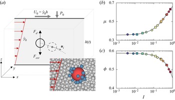
The flow consists of a three-dimensional streamwise ( $x$) and spanwise (
 $y$) periodic domain confined by two rough walls in the depthwise (
 $z$) direction (figure 1a), where the walls are roughened by randomly distributed stationary particles (Jing et al. Reference Jing, Kwok, Leung and Sobral2016). The lower wall is stationary, while the upper wall translates in
 $x$ with a velocity
 $U_0=\dot \gamma _0 h$, where
 $\dot \gamma _0$ is the shear rate and
 $h=h(t)$ is the instantaneous flow depth which varies slightly in time
 $t$, and is reactive in
 $z$ to maintain a constant overburden pressure
 $P_0$. Gravity is not present (
 $g=0$) in simple shear simulations, but we show below that our findings remain valid when gravity is included. The domain is typically
 $20d$ long,
 $20d$ wide and
 $35d$ deep (approximately
 $15\,000$ spherical particles per simulation), where
 $d$ is the mean bed particle diameter (with
 $\pm 10\,\%$ uniform polydispersity). We have increased the domain size to confirm that it is sufficiently large to avoid boundary effects.
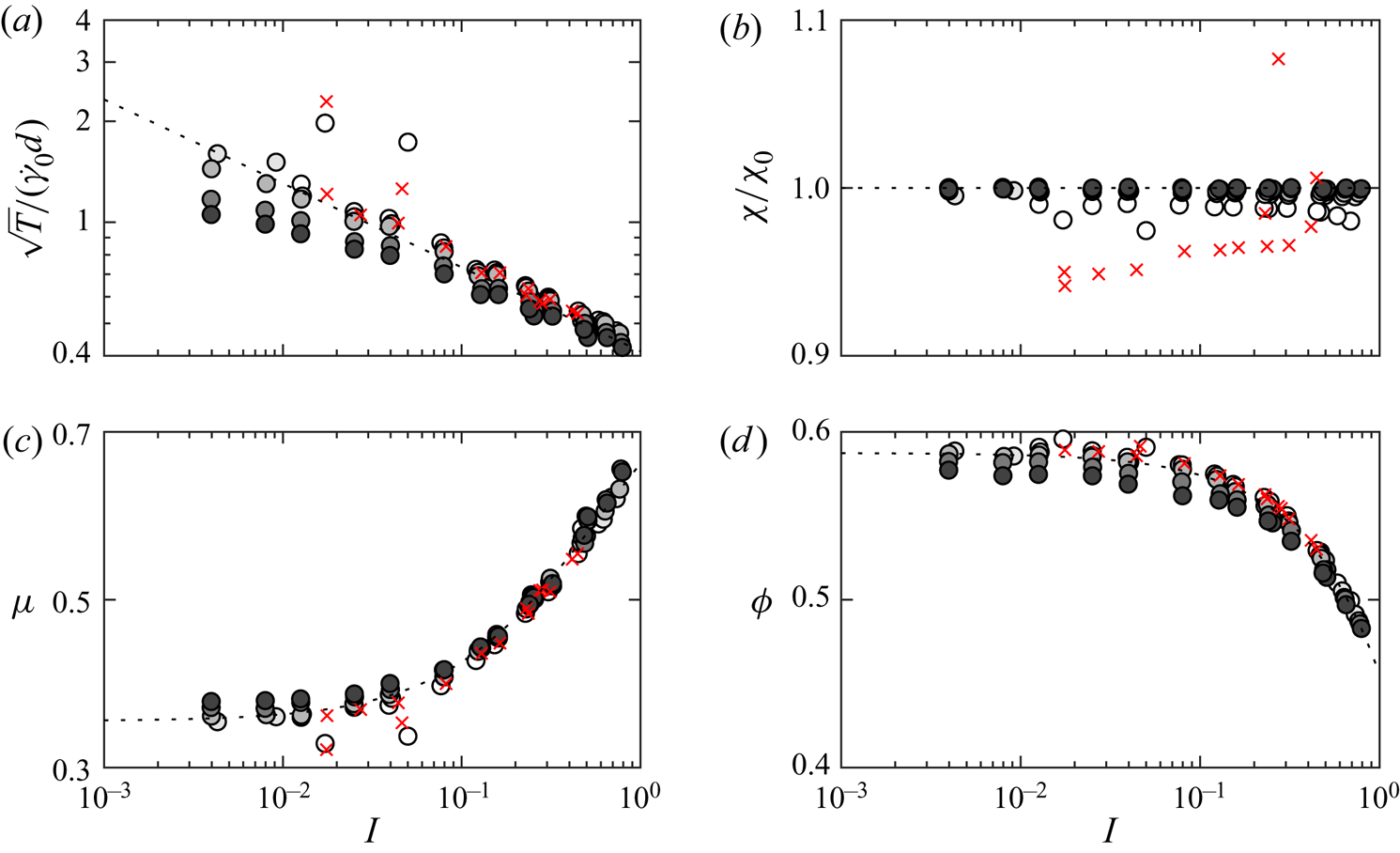
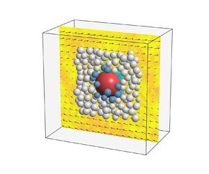
(a) Simulation set-up and schematic trajectory of an intruder particle (not to scale). The inset shows a sinking intruder (red) and its contacting (blue) and non-contacting (grey) neighbouring particles in a small section of the flow. (b,c) Rheological data measured in the flow for  $10\leqslant z/d \leqslant 20$ for various simulations. Square and circle symbols represent
 $P_0=100$ Pa and
 $1000$ Pa, respectively, and the colour from blue to red indicates increasing
 $I$ (see text for range of
 $\dot \gamma _0$). Solid curves in (b) and (c) are described by
 $\mu (I)=0.36+0.55/(0.73/I+1)$ and
 $\phi (I)=0.59-0.14I$, respectively.

To ensure homogeneous shear in each simulation, which does not otherwise occur under all simulation conditions due to possible shear localization near the moving wall, we apply a small streamwise stabilizing force  $F_s=K_s[u(z_p)-u_p]$ to each particle (except the intruder particle) at each DEM simulation time step to maintain the desired linear flow velocity profile,
 $u(z)=\dot \gamma _0 z$, where
 $u_p$ and
 $z_p$ are instantaneous particle velocity and position, respectively, and
 $K_s$ is a constant (Lerner, Düring & Wyart Reference Lerner, Düring and Wyart2012; Clark et al. Reference Clark, Thompson, Shattuck, Ouellette and O'Hern2018; Fry et al. Reference Fry, Umbanhowar, Ottino and Lueptow2018; Jing et al. Reference Jing, Ottino, Lueptow and Umbanhowar2020, Reference Jing, Ottino, Lueptow and Umbanhowar2021). The appropriate value of
 $K_s$ to avoid altering the granular flow rheology and yet ensure a linear velocity profile depends on
 $P_0$ and
 $\dot \gamma _0$ (Fry et al. Reference Fry, Umbanhowar, Ottino and Lueptow2018). We provide a detailed scaling analysis of
 $K_s$ in Appendix A. Based on that analysis, we set the dimensionless version of this parameter to be
 $\tilde {K}_s = K_s\dot \gamma _0I^{-0.25}/(P_0d) = 0.1$ for all simulations, where
 $I=\dot \gamma _0 d/\sqrt {P_0/\rho }$ is the inertial number and
 $\rho$ is the particle density. This choice produces satisfactorily homogeneous flows while not altering the flow rheology and drag behaviours; increasing or decreasing
 $\tilde {K}_s$ by a factor of 10 does not affect the results (see Appendix A).
We focus on the dense granular flow regime, characterized by the inertial number  $I$ ranging approximately from
 $10^{-3}$ to
 $1$, to avoid possible non-local effects for
 $I \lesssim 10^{-3}$ (Kim & Kamrin Reference Kim and Kamrin2020) and the dilute, collisional flow regime for
 $I \gtrsim 1$ (Rognon & Macaulay Reference Rognon and Macaulay2021). To achieve this range of
 $I$, we use
 $\dot \gamma _0=\{0.5,1,5,10,20,30,40,60,80\}$ s
 $^{-1}$ for
 $P_0=1000$ Pa and
 $\dot \gamma _0=\{0.5,1,5,10,20,30\}$ s
 $^{-1}$ for
 $P_0=100$ Pa. Bed particle properties are
 $d=5$ mm and
 $\rho =2500$ kg m
 $^{-3}$, but we vary
 $d$ and
 $\rho$ to confirm the scaling associated with
 $I$. Figure 1(b,c) show the rheological data, including the effective friction
 $\mu$ and average solid packing density
 $\phi$, measured in a
 $10d$-thick layer in the middle of the flow, which follow the
 $\mu (I)$ and
 $\phi (I)$ relations typical of dense granular flows (Forterre & Pouliquen Reference Forterre and Pouliquen2008). For the DEM simulations, we use the Hertz contact model with Young's modulus
 $5\times 10^7$ Pa, Poisson's ratio
 $0.4$, coefficient of restitution
 $0.8$ and coefficient of friction
 $0.5$. Note that using a linear contact model should produce similar results based on previous studies using the model for segregation in dense granular flows (Jing et al. Reference Jing, Ottino, Lueptow and Umbanhowar2020; Duan et al. Reference Duan, Jing, Umbanhowar, Ottino and Lueptow2022). The simulation time step is
 $10^{-5}$ s to assure numerical stability, and the results are insensitive to the contact parameters except for particle friction coefficients
 $\lesssim 0.3$, in agreement with previous studies (Tripathi & Khakhar Reference Tripathi and Khakhar2011; Duan et al. Reference Duan, Umbanhowar, Ottino and Lueptow2020; Jing et al. Reference Jing, Ottino, Lueptow and Umbanhowar2020; Bancroft & Johnson Reference Bancroft and Johnson2021).
2.2. Intruder particles and drag measurement
We study drag on a small number of spherical intruder particles in the flow (see figure 1a), with a range of size ratios  $R=d_i/d$ from
 $0.6$ to
 $5$ and density ratios
 $R_\rho =\rho _i/\rho$ from
 $1$ to
 $20$, where
 $d_i$ and
 $\rho _i$ are the intruder diameter and density, respectively. Typically, five intruders are included in each simulation to obtain statistically significant results, and we verify that the intruders are far enough apart that they do not interact with each other, a situation shown to occur at intruder particle concentrations below a finite critical concentration (Duan et al. Reference Duan, Jing, Umbanhowar, Ottino and Lueptow2022). However, for
 $R>2$, the domain size needs to be at least doubled compared with that for
 $R=1$ to accommodate multiple non-interacting intruders (Pacheco-Vázquez & Ruiz-Suárez Reference Pacheco-Vázquez and Ruiz-Suárez2010), which is computationally expensive, so we only use one intruder per simulation for
 $R>2$. Nevertheless, we confirm that this is statistically sufficient because fluctuations associated with the random action of particle contacts decreases significantly for large
 $R$ due to the rapid increase in the number of contacts with the intruder (which grows as
 $R^2$).
Each intruder is dragged by a constant external force  $F_{ext}$ imposed in the negative
 $z$-direction but is free to move with the flow in the
 $x$- and
 $y$-directions, as illustrated in figure 1(a). We have verified that dragging the intruder upward (in the absence of gravity) produces similar results. The net resistive drag force,
 $F_d$, i.e. the net force exerted on the intruder by bed particle contacts in the
 $z$-direction, is simply
 $F_d=F_{ext}$. The force balance is justified because the intruder migration is, on average, always in equilibrium; that is, we observe negligible net intruder acceleration in all simulations. For each applied
 $F_{ext}$, the corresponding mean (downward) intruder velocity,
 $w_i$, is determined based on the vertical trajectories of all intruders in a simulation as they pass through the flow depth from
 $z=20d$ to
 $10d$ (typically encompassing approximately
 $50$ snapshots over the time for the intruder to transit this distance; see plots of the intruder position versus time in § 3.1), thereby avoiding effects related to the lower or upper walls (Stone et al. Reference Stone, Bernstein, Barry, Pelc, Tsui and Schiffer2004). Then, we analyse the relationship between
 $F_d$ and
 $w_i$ for a series of simulations with varying
 $F_{ext}$. Note that
 $F_d$ acts in the opposite direction to
 $w_i$, but the signs of
 $F_d$ and
 $w_i$ are omitted here for simplicity. The situation is analogous to the relation between the drag force on a particle sedimenting in a static fluid and its terminal velocity, except that here the external force is imposed (rather than a result of gravity) and the granular bed flows with a uniform shear rate. Furthermore, we note that an intruder particle in a granular shear flow may experience shear-induced lift effects due to possible velocity differences (i.e. slip velocity) between the intruder and the nearby mean flow in the streamwise direction (van der Vaart et al. Reference van der Vaart, van Schrojenstein Lantman, Weinhart, Luding, Ancey and Thornton2018). Therefore, the effective drag force
 $F_d$ defined in this paper, similar to previous work (Tripathi & Khakhar Reference Tripathi and Khakhar2011; Liu & McCarthy Reference Liu and McCarthy2017; Duan et al. Reference Duan, Umbanhowar, Ottino and Lueptow2020; Bancroft & Johnson Reference Bancroft and Johnson2021), simply represents the net resistive force on the intruder in the
 $z$-direction and, although different mechanisms contribute to
 $F_d$, our focus is the relation between
 $F_d$ and
 $w_i$ for various simulation conditions.
Following this procedure, we first vary  $F_{ext}$ over four orders of magnitude to explore possible drag regimes and identify the transition from viscous-like to inertial-like regimes. Then, focusing on the viscous regime, we develop a general scaling law for the drag force based on a comprehensive parametric study for different combinations of flow conditions (
 $P_0$ and
 $\dot \gamma _0$, hence
 $I$) and intruder properties (
 $R$ and
 $R_\rho$). In total, results for over
 $1000$ simulations are reported for the drag study. Finally, an additional set of approximately
 $80$ simulations with gravity (
 $g=9.81$ m s
 $^{-2}$) are conducted to explore the ability of our drag model, together with a previous segregation force model (Jing et al. Reference Jing, Ottino, Lueptow and Umbanhowar2020), to predict the intruder velocity in gravity-driven size and density segregation.
3. Results
3.1. Typical drag behaviours ( $R=1$ and $R_\rho =1$)


We first consider applying  $F_{ext}$ to five intruder particles having the same size and density as the bed particles (
 $R=1$ and
 $R_\rho =1$). The drag force (or, equivalently, the applied driving force
 $F_{ext}$) is non-dimensionalized as
 $F_d/(P_0d_i^2)$ since
 $P_0d_i^2$ is the only intrinsic (contact) force scale in this dense, simple shear flow, where gravity is not present and the contact pressure dominates over the kinetic pressure. In figure 2(a–d), four widely varying values of
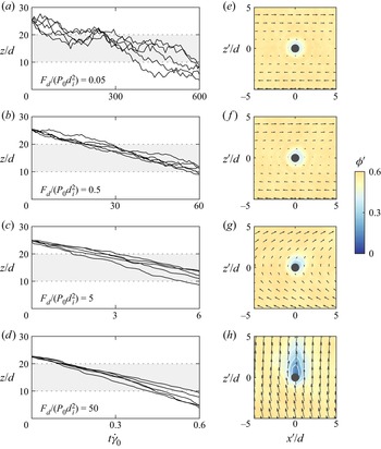
 $F_d/(P_0d_i^2) = \{0.05, 0.5, 5, 50\}$ are used to show examples of the intruder position in
 $z$ versus time
 $t$, which are non-dimensionalized by the bed particle diameter
 $d$ and the shear rate
 $\dot \gamma _0$, respectively. The flow inertial number is
 $I=0.08$ (
 $P_0=1000$ Pa and
 $\dot \gamma _0=10$ s
 $^{-1}$). Note that
 $t=0$ in figure 2 denotes the time when
 $F_{ext}$ is first applied on the intruder, prior to which the flow and the intruder are at steady state (for
 $t<0$, the intruder is allowed to move with the flow but is vertically constrained at its initial height by a virtual spring – see Jing et al. (Reference Jing, Ottino, Lueptow and Umbanhowar2021)).
Examples of (a–d) intruder vertical position versus time  $t$ and (e–h) corresponding flow fields around the intruder (in the intruder reference frame) for various drag forces
 $F_d$ (see labels in the figure; note the differing horizontal time scales). The flow conditions are
 $P_0=1000$ Pa and
 $\dot \gamma _0=10$ s
 $^{-1}$ (
 $I=0.08$), and the intruder properties are
 $R=1$ and
 $R_\rho =1$. Grey areas in (a–d) indicate the measurement window where the intruder velocity (slope) and local flow fields are evaluated (see §§ 2.2 and 3.1 for details). The white contours of local packing density
 $\phi '$ in (e–h) have an interval of
 $0.1$ and the outermost contour is for
 $\phi '=0.5$. For clarity, the velocity vectors are presented at a coarser resolution than the
 $\phi '$ fields and the arrows in (e–h) have different scales; the scale of
 $w_i$ can be roughly inferred from figure 3.

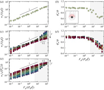
Drag force results for intruders equal in size and density to the surrounding bed particles ( $R=1$ and
 $R_\rho =1$). (a) Intruder velocity
 $w_i/(\dot \gamma _0d_i)$ and (b) nearby packing density
 $\phi '_n/\phi$ versus drag force
 $F_d/(P_0d_i^2)$ for
 $P_0=1000$ Pa and
 $\dot \gamma _0=10$ s
 $^{-1}$ (
 $I=0.08$). The shaded red area in the inset of (b) indicates the region where
 $\phi '_n$ is evaluated. Panels (c,d) are the same as (a,b) but for all flow conditions (same symbols as in figure 1). Panel (e) is the same as (c) except that
 $w_i$ is non-dimensionalized by
 $\sqrt {P_0/\rho }$ instead of
 $\dot \gamma _0d_i$. Grey shaded areas in (b–e) indicate the approximate conditions (
 $F_d/(P_0d_i^2)\gtrsim 5$) where cavity formation is significant (
 $\phi '_n/\phi \lesssim 0.9$).

Figure 2(a) shows that when  $F_d$ is much smaller than the typical contact force magnitude (
 $F_d/(P_0d_i^2)=0.05$), the intruder vertical position exhibits significant fluctuations and, occasionally, the intruder lingers around a certain flow depth or even rises briefly before continuing its downward trajectory (see also supplementary movie 1 which is available at https://doi.org/10.1017/jfm.2022.706). This intermittency of the downward intruder migration due to a very small driving force is somewhat reminiscent of the subyielding behaviour of granular drag (Zheng et al. Reference Zheng, Wang, Barés and Behringer2018) and is likely a consequence of random particle collisions acting on the intruder. Nevertheless, an overall trend of downward intruder migration is observed in the measurement window of
 $10\leqslant z/d \leqslant 20$ (shaded area in figure 2a) and, therefore, a mean velocity
 $w_i$ can be calculated as detailed in § 2.2 and discussed in the subsequent analysis. Figure 2(b–d) show the temporal evolution of the intruder vertical position for three larger drag forces,
 $F_d/(P_0d_i^2)=\{0.5,5,50\}$, respectively, which exhibit qualitatively similar trends as in figure 2(a) but with increasingly smaller fluctuations. Note that the horizontal time scale decreases by a factor of 10 as
 $F_d/(P_0d_i^2)$ is increased by 10 times, indicating a (linearly) increasing velocity with increasing
 $F_d/(P_0d_i^2)$. The mean intruder acceleration in the observation window is negligible, as is evident for the cases in figure 2(b–d), for the full range of
 $F_d$ that we explore, indicating that the particles around the intruder react to the intruder migration such that a local quasi-equilibrium occurs with
 $F_{ext}$ balanced by
 $F_d$.
To further explore the interaction between the intruder and its surrounding particles for these four example simulations, we visualize the corresponding mean flow fields around the intruder (filled circles) in figure 2(e–h), which include the local packing density  $\phi '$ (coloured surface plots and white contours) and the relative flow velocity (arrows)
 $\boldsymbol {u}'=\boldsymbol {u}-\boldsymbol {u}_i$, where
 $\boldsymbol {u}$ and
 $\boldsymbol {u}_i$ are the flow and intruder velocity vectors, respectively. For each intruder, the surrounding flow fields are evaluated within a
 $10d\times 1d\times 10d$ cross-section centred at the intruder position
 $(x_i,y_i,z_i)$ with a local coordinate system
 $(x',y',z')=(x-x_i,y-y_i,z-z_i)$. In this subdomain, particle positions and velocities are first mapped onto a set of
 $0.2d\times 1d\times 0.2d$ grids, then smoothed via a disk filter (radius of
 $d$) in the
 $x'z'$-plane, and finally averaged over all output frames in the observation window for all five intruders. As figure 2(e) shows, when the drag force is very small (
 $F_d/(P_0d_i^2)=0.05$), the flow around the intruder is dominated by the primary shear flow in
 $x'$ with negligible relative velocities in
 $z'$, and the disturbance of the intruder on the packing density of the surrounding particles is negligible, although the contours of
 $\phi '$ show an excluded volume effect that is symmetric about the intruder, as expected (Tripathi & Khakhar Reference Tripathi and Khakhar2011). The flow pattern for
 $F_d/(P_0d_i^2)=0.5$ (figure 2f) is similar to that for
 $F_d/(P_0d_i^2)=0.05$, but the velocity vectors display a small component in the
 $z'$-direction due to increasing relative velocity in
 $z'$. This becomes more evident when the drag force is increased to
 $F_d/(P_0d_i^2)=5$ (figure 2g), where the induced relative velocity in
 $z'$ is approximately of the same order of that in
 $x'$, and a semicircular flow pattern is formed around the intruder, consistent with the shear flow relative to the intruder (rightward above the intruder and leftward below). Moreover, an asymmetric packing structure emerges with a decrease in the packing density (low
 $\phi '$ zone) above the intruder, essentially in the ‘wake’ of the downward moving intruder (see also supplementary movie 2). Lastly, for the largest drag force,
 $F_d/(P_0d_i^2)=50$ (figure 2h), the relative velocity in
 $z'$ dominates because the intruder velocity is much larger than the velocity associated with the shear. In addition, a significant teardrop-shaped cavity (where
 $\phi '$ can be as low as zero) appears behind the intruder, indicating that the downward migration of the intruder is fast enough that the nearby particles cannot rearrange themselves quickly enough to refill the gap, resulting in a cavity behind the intruder. The significant changes in the local flow pattern and packing structure in figure 2(e–h) beg the question of how they might affect the scaling of
 $F_d$, which is described in the next subsection.
3.2. Drag force regimes ($R=1$ and $R_\rho =1$)


To characterize the regimes of the drag force, the intruder velocity  $w_i/(\dot \gamma _0d_i)$, averaged over five intruder particles for each condition, is plotted in figure 3 against the corresponding drag force
 $F_d/(P_0d_i^2)$ for intruders having the same size and density as the surrounding particles (
 $R=1$ and
 $R_\rho =1$). The velocity is non-dimensionalized based on the shear time scale (
 $\dot \gamma _0$) and the intruder size (
 $d_i$), although non-dimensionalization using a velocity scale for the bed particle rearrangement (
 $\sqrt {P_0/\rho }$) is also considered.
Figure 3(a) presents the results of  $21$ simulations for varying
 $F_d/(P_0d_i^2)$ that have the same flow conditions as those in figure 2, i.e.
 $I=0.08$ (
 $P_0=1000$ Pa and
 $\dot \gamma _0=10$ s
 $^{-1}$). A linear relationship between
 $w_i/(\dot \gamma _0d_i)$ and
 $F_d/(P_0d_i^2)$ (i.e. a viscous-like regime) is found over a wide range of intermediate
 $F_d/(P_0d_i^2)$ values. For very small forces,
 $F_d/(P_0d_i^2)=O(10^{-2})$, scatter of the data increases (error bars are not shown as they are generally smaller than the symbols) due to increased fluctuations and intermittency in the temporal evolution of the intruder vertical position, as shown in figure 2(a). For very large forces,
 $F_d/(P_0d_i^2)=O(10)$, the slope of the curve deviates slightly from unity, which we attribute to the inertial effect of cavity formation as shown in figure 2(h). Furthermore, to quantitatively identify the transition between the viscous and inertial regimes, we plot a local packing density in the wake of the intruder
 $\phi _n'/\phi$ against
 $F_d/(P_0d_i^2)$ in figure 3(b), which starts to drop significantly below unity when
 $F_d/(P_0d_i^2)$ exceeds approximately five due to cavity formation. Here,
 $\phi _n'$ is the mean value of
 $\phi '$ within a nearby semicircular annular region located above the intruder having an arbitrary outer radius
 $1.5d_i$ from the centre of the intruder, as illustrated in the inset of figure 3(b), and the normalization of
 $\phi _n'/\phi$ eliminates the influence of
 $I$ on the average packing density
 $\phi$ (see figure 1c).
Figures 3(c) and 3(d) show the results of  $315$ simulations (
 $R=1$ and
 $R_\rho =1$) for all the flow conditions that we explore (characterized by
 $I$), where the symbol colours and shapes match those in figure 1(b,c). Several key observations can be made. First, the transitional behaviours related to intermittent intruder migration at the low end and cavity formation at the high end for the curves in figure 3(c) are similar despite the wide range of
 $I$ (from
 $0.004$ to
 $0.75$). In particular, all curves are linear (slope one) in an intermediate range of
 $F_d/(P_0d_i^2)$, approximately between
 $0.1$ and
 $5$, indicating a viscous scaling for the drag force,
 $F_d/(P_0d_i^2) \propto w_i/(\dot \gamma _0d_i)$, or
 $F_d\propto (P_0/\dot \gamma _0)d_iw_i$, which corresponds to the example intruder dynamics in figure 2(b,c). Outside this viscous-like regime, data scatter grows for
 $F_d/(P_0d_i^2)\lesssim 0.1$, making it hard to accurately characterize the
 $F_d$ versus
 $w_i$ relation due to the increasing fluctuations and intermittency of the intruder migration (figure 2a), and a change of slope occurs for
 $F_d/(P_0d_i^2)\gtrsim 5$ due to inertial effects such as the cavity formation in figure 2(h). Second, in the inertial regime (
 $F_d/(P_0d_i^2)\gtrsim 5$), the slopes of the curves show non-trivial dependence on
 $I$, which is clarified below with respect to figure 3(e); nevertheless, it is evident that the curves for high inertial numbers (red symbols) approach a slope of
 $1/2$, indicating the familiar quadratic scaling
 $F_d\propto w_i^2$ for inertial drag of collisional granular flows (Jenkins & Yoon Reference Jenkins and Yoon2002; Seguin & Gondret Reference Seguin and Gondret2017; Das, Puri & Schwartz Reference Das, Puri and Schwartz2020). Finally, as a signature of the transition from the viscous regime to the inertial regime, significant cavity formation occurs in the wake of the intruder when
 $F_d/(P_0d_i^2)\gtrsim 5$, regardless of
 $I$ (i.e. rapid drop of
 $\phi '_n/\phi$ in figure 3d), which suggests a threshold value beyond which the contact forces that drive particle rearrangement (which scale with
 $P_0d^2$) are inadequate to quickly fill the wake behind the intruder.
The diverging slopes of the curves for  $F_d/(P_0d_i^2)\gtrsim 5$ in figure 3(c) are a result of the chosen velocity scale,
 $w_i/(\dot \gamma _0d_i)$. Indeed,
 $w_i$ is expected to be independent of
 $\dot \gamma _0$ in the inertial regime, where the intruder transits downward so rapidly that the shear is negligible in the intruder reference frame – see figure 2(h). Instead, a relevant velocity scale that determines how fast the bed particles rearrange near the intruder is
 $\sqrt {P_0/\rho }$. Figure 3(e) shows the rescaled intruder velocity
 $w_i/\sqrt {P_0/\rho }$ versus
 $F_d/(P_0d_i^2)$, indicating a clear convergence of all curves to the highest-
 $I$ curve and towards the same slope of
 $1/2$ in the inertial regime (shaded area). This leads to an inertial drag force scaling of
 $F_d/(P_0d_i^2) \propto (w_i/\sqrt {P_0/\rho })^2$, or
 $F_d \propto \rho d_i^2 w_i^2$. Interestingly, the transition of the slope from one to
 $1/2$ is more direct for high-
 $I$ cases (red symbols) than low-
 $I$ cases (blue symbols), perhaps because when
 $I$ is low (
 $I\lesssim 0.01$), where the bed deformation is otherwise quasistatic (Azéma & Radjaï Reference Azéma and Radjaï2014), the intruder needs to sufficiently fluidize the nearby bed particles such that its migration behaviour transitions from the viscous to inertial regimes. Another interesting observation in figure 3(e) is that the curves do not collapse in the viscous regime (
 $F_d/(P_0d_i^2)\lesssim 5$) when
 $w_i$ is scaled by
 $\sqrt {P_0/\rho }$, in contrast to the data collapse in figure 3(c) where
 $w_i$ is scaled by
 $\dot \gamma _0d_i$. This justifies our choice of the dimensionless velocity
 $w_i/(\dot \gamma _0d_i)$ throughout this paper, since the intruder drag is mainly in the viscous-like regime.
3.3. Viscous-like drag force scaling ($R=1$ and $R_\rho =1$)


The results in figure 3 show that the drag force follows a viscous-like scaling ( $F_d \propto w_i$) over a wide range of
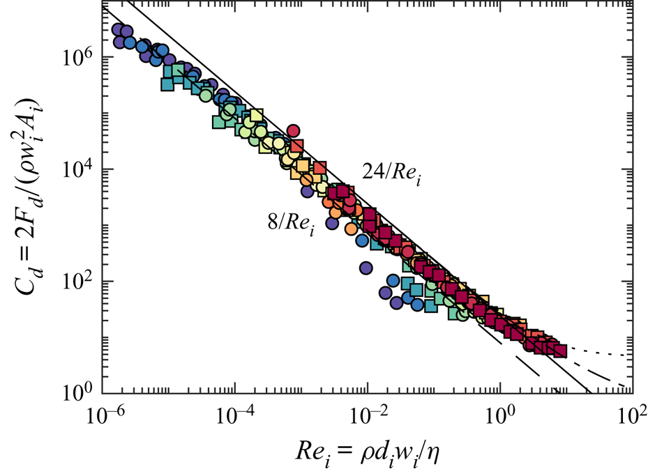
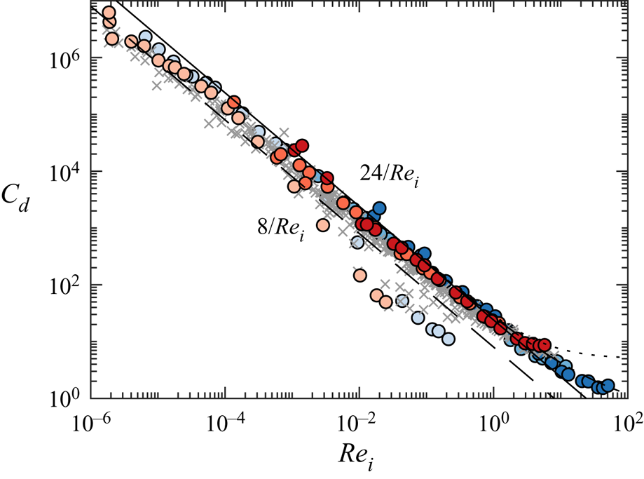
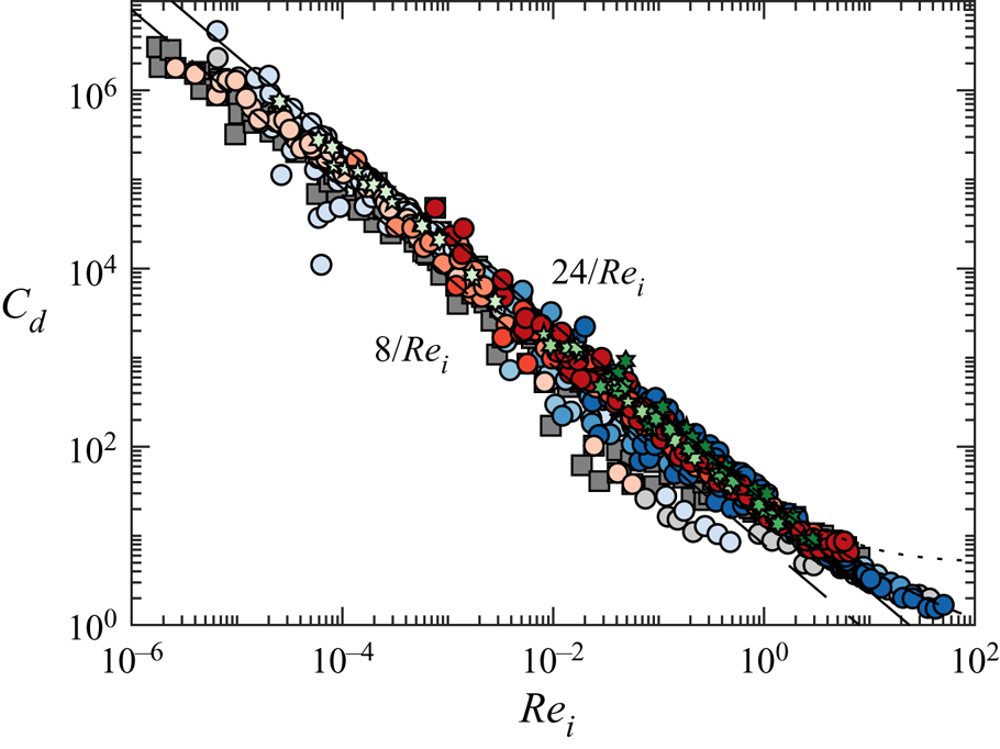
 $F_d/(P_0d_i^2)$, which is reminiscent of the Stokes regime for the drag of a sphere in a uniform flow of a viscous fluid. To demonstrate this analogy more quantitatively, we recast the data in figure 3(c) as the drag coefficient,
 $C_d$, versus the intruder Reynolds number,
 $Re_i$, in figure 4, as is often done for the drag on a sphere in a fluid. Here,
 $C_d=2F_d/(\rho w_i^2 A_i)$,
 $A_i={\rm \pi} d_i^2/4$,
 $Re_i=\rho d_i w_i/\eta$ and
 $\eta =\mu P_0/\dot \gamma _0$ is the effective granular flow viscosity with
 $\mu =\mu (I)$ described by the curve in figure 1(b). The data fall onto a master curve with a slope of
 $-1$ in figure 4. The viscous relation
 $C_d \propto 1/Re_i$ extends over a surprisingly wide range of
 $Re_i$ from
 $10^{-5}$ to
 $1$. Deviations from this viscous relation occur for
 $Re_i<10^{-5}$ and
 $Re_i>1$, respectively, due to the fluctuation- and inertia-related effects discussed above; only a few data points (bluish data points below the dashed line) deviate from the master curve due to the transitional behaviour from slope one to slope
 $1/2$ for low-
 $I$ cases (
 $I\lesssim 0.01$), as discussed above regarding figure 3(e).
Drag coefficient  $C_d$ versus intruder Reynolds number
 $Re_i$ for
 $R=1$ and
 $R_\rho =1$. Data are recast from figure 3(c) with the same symbols. The solid, dashed, dotted and dot–dash curves represent relations
 $C_d=24/Re_i$,
 $C_d=8/Re_i$,
 $C_d=24/Re_i(1+3Re_i/16)$ and
 $C_d=24/Re_i+6/(1+\sqrt {Re_i})+0.4$, respectively (see text).

In figure 4, we further indicate the  $C_d=24/Re_i$ (total drag, solid curve) and
 $C_d=8/Re_i$ (form drag, dashed curve) relations (see, e.g. White Reference White1974) to directly compare our ‘granular drag’ data with Stokes’ viscous drag for a sphere. Our data falls between these two limiting cases, indicating a form for the granular drag coefficient,
 $C_d=8c/Re_i$, where
 $c$ is a prefactor ranging approximately from
 $1$ to
 $3$ (i.e. bounded by the dashed and solid curves). Alternatively, this is rewritten as a Stokes-like drag force,
 \begin{equation} F_d=c{\rm \pi}\eta d_iw_i, \end{equation}
where the prefactor  $c$ depends somewhat on simulation conditions (see § 3.4). Note that, as mentioned in § 2.2, the signs of
 $F_d$ and
 $w_i$ are omitted for brevity, although
 $F_d$ is opposite to
 $w_i$. Expression (3.1) is precisely the Stokes drag model for a sphere in a viscous fluid if
 ${c=c_{St}}$, where
 $c_{St}=3$ is the sum of the form drag (
 $c_{St}/3$) and the friction drag (
 $2c_{St}/3$) (White Reference White1974). Although we make no claim of a direct analogy, it is interesting that the prefactor
 $c$ in a dense granular flow varies from
 ${c_{St}/3=1}$ (form drag) to
 ${c_{St}=3}$ (total drag), which highlights the subtle differences between dissipation due to particle interactions in a granular flow and that due to viscosity in a fluid. Moreover, we have verified that the DEM contact parameters do not affect the
 $C_d$ versus
 $Re_i$ results (as noted in § 2.1), consistent with previous results (Tripathi & Khakhar Reference Tripathi and Khakhar2011; Bancroft & Johnson Reference Bancroft and Johnson2021). This further indicates that granular drag is the collective consequence of particle interactions typical of dense granular flows.
Finally, it is also interesting to note that, for  $Re_i>1$, the data tends to level off with increasing
 $Re_i$, similar to the non-Stokesian drag behaviour of a sphere in a fluid due to inertia-related effects (Goossens (Reference Goossens2019), and references therein). To further demonstrate this, in figure 4, we plot both Oseen's drag model (Schlichting Reference Schlichting1979),
 $C_d=24/Re_i(1+3Re_i/16)$, which is strictly valid only for
 $Re_i<5$ (dotted curve), and the empirical fit by White (White Reference White1974),
 $C_d=24/Re_i+6/(1+\sqrt {Re_i})+0.4$ (dot–dash curve). Both relations suggest that the similarity between the drag on a spherical particle in a granular flow and the drag on a sphere in a fluid extends beyond the viscous Stokes flow regime (
 $Re_i\lesssim 1$) into the inertial flow regime.
We caution here that the analogy with drag on a sphere in a fluid is imperfect. For a sphere in a fluid, the drag force is based on moving the sphere through a quiescent fluid (or, equivalently, a uniform fluid flow over a stationary sphere). As a result, there is no lift force. The situation differs here in that the spherical intruder particle is moved through a sheared granular medium (i.e. transiting through regions with decreasing mean flow velocities) so that we can connect these drag results to those for segregating particles in sheared granular flows, as in previous work on this topic (Tripathi & Khakhar Reference Tripathi and Khakhar2011; Liu & McCarthy Reference Liu and McCarthy2017). However, the uniform shear velocity field may lead to lift forces when there is a slip velocity between the intruder and the sheared bed. Hence, the drag force we measure is essentially the ‘net resistive drag force’, which may include effects related to the effective streamwise slip of the intruder relative to the shear flow, as discussed later in this paper.
3.4. Drag force for varying $R$ and $R_\rho$


To investigate the effects of the intruder size ratio  $R=d_i/d$ and density ratio
 $R_\rho =\rho _i/\rho$ on the drag force, we vary
 $d_i$ and
 $\rho _i$, respectively, for various
 $I$. Figure 5 presents two representative scenarios with
 $R=4$ and
 $R_\rho =1$ (blue symbols) and with
 $R=1$ and
 $R_\rho =10$ (red symbols), where the degree of colour saturation from light to dark indicates the three values of
 $I=\{0.004,0.16,0.64\}$; the results from figure 3 (with
 $R=1$ and
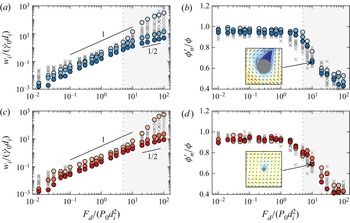
 $R_\rho =1$) are reproduced as grey crosses in figure 5 for comparison. As figure 5(a) shows, when
 $R=4$, the basic drag characteristics (linear and nonlinear regimes) for various
 $I$ are similar to those for
 $R=1$, but the curves are shifted downward, indicating that a larger drag force is needed to achieve the same intruder velocity. The shift is the consequence of a stronger disturbance in the flow as the larger intruder transits through the flow, which is evident in the larger low-density area around the intruder in the inset of figure 5(b) (see also supplementary movie 3). Interestingly, the transition of
 $\phi '_n/\phi$ for
 $R=4$ is similar to that for
 $R=1$ (see figure 5b), indicating that under the same
 $F_d/(P_0 d_i^2)$ the cavity shape is similar for different
 $R$, although the cavity size scales approximately with the cross-sectional area of the intruder. Moreover, the effect of
 $R$ on the
 $F_d$ versus
 $w_i$ scaling (figure 5a) is even smaller than that on the near-intruder flow density (figure 5b), indicating again that the intruder drag originates mainly from particle interactions at its leading edge but is less affected by the cavity area in its wake. Perhaps more important is that the
 $w_i/(\dot \gamma _0 d_i)$ versus
 $F_d/(P_0 d_i^2)$ relation remains linear in the same range of
 $F_d/(P_0 d_i^2)$ as for
 $R=1$, and that, although not shown, the
 $w_i/\sqrt {P_0/\rho }$ versus
 $F_d/(P_0 d_i^2)$ relation transitions towards slope
 $1/2$ for large
 $F_d/(P_0 d_i^2)$, similar to the
 $R=1$ results in figure 3(e).
Effects of larger size ratio ( $R=4$ and
 $R_\rho =1$, blue symbols, panels (a,b)) and larger density ratio (
 $R=1$ and
 $R_\rho =10$, red symbols, panels (c,d)) on (a,c)
 $w_i/(\dot \gamma _0d_i)$ versus
 $F_d/(P_0d_i^2)$ and (b,d)
 $\phi '_n/\phi$ versus
 $F_d/(P_0d_i^2)$ results. Light, medium and dark colours correspond to
 $I=\{0.004,0.16,0.64\}$, respectively, and grey crosses are
 $R=1$ and
 $R_\rho =1$ data reproduced from figure 3(b,d) for comparison. Insets in (b,d) at
 $F_d/(P_0d_i^2)=10$ and
 $I=0.64$ demonstrate the near-intruder flow fields using the same colour map as figure 2(e–h). Grey shaded areas match those in figure 3(b–e).

The results for  $R_\rho =10$ show that the influence of the intruder density on the
 $w_i/(\dot \gamma _0 d_i)$ versus
 $F_d/(P_0 d_i^2)$ relation (figure 5c) and the flow field around the intruder (figure 5d) are less significant than the intruder size effects at
 $R=4$, although a slightly lower intruder velocity is observed for large
 $F_d/(P_0 d_i^2)$ cases in the more collisional flow (
 $I=0.64$), indicating a slightly larger drag force (figure 5c). The effects of
 $R$ and
 $R_\rho$ on the drag force is discussed in greater detail in § 3.5.
Figure 6 shows that recasting the data in figure 5(a,c) into the  $C_d$ versus
 $Re_i$ form leads to results that remain bounded by the
 $8/Re_i$ and
 $24/Re_i$ scaling, except for a few cases related to the transitional behaviour of low-
 $I$ cases (similar to figure 4). Therefore, as a first-order approximation, the drag force on a spherical particle (
 $1\leqslant R \leqslant 4$ with
 $R_\rho =1$ and
 $1\leqslant R_\rho \leqslant 10$ with
 $R=1$) in a dense granular flow (
 $10^{-3}\lesssim I \lesssim 1$) can be estimated by a Stokesian drag coefficient
 $C_d = 8c/Re_i$, where
 $c$ ranges approximately from
 $1$ to
 $3$, for a wide range of intruder Reynolds numbers (
 $10^{-5} \lesssim Re_i \lesssim 1$). For larger Reynolds numbers (
 $1 \lesssim Re_i \lesssim 100$), the data indicate that
 $C_d$ deviates from this relation due to inertial effects, following the Oseen approximation for
 $R_\rho =10$ and the White empirical fit for
 $R=4$ (figure 6). While this result is interesting, we do not explore it further in this paper.


3.5. Dependence of drag prefactor $c$ on parameters

Despite the data collapse to a master curve  $C_d = 8c/Re_i$ in figures 4 and 6, it is evident that the prefactor
 $c$ exhibits (secondary) dependence on the flow condition (
 $I$) and the intruder properties (
 $R$ and
 $R_\rho$), i.e.
 $c=c(I,R,R_\rho )$. To further examine this dependence, we use the drag force expression (3.1) to obtain the mean value of
 $c=F_d/({\rm \pi} \eta d_iw_i)$ for a given set of (
 $I,R,R_\rho$) conditions – see figure 7. Note that, to focus on the linear regime (
 $F_d \propto w_i$), we only consider the
 $F_d$ versus
 $w_i$ data associated with
 $0.1 \leqslant F_d/(P_0d_i^2) \leqslant 5$ according to the discussion with respect to figure 3. Each value for
 $c$ plotted in figure 7 represents an average over six to nine simulations (in total, approximately
 $800$ simulations); unaveraged data can be found in figure 9 (which includes all simulation conditions) and the figure in Appendix C (which only includes simulations with
 $0.1 \leqslant F_d/(P_0d_i^2) \leqslant 5$).
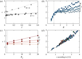
Dependence of  $c$ on
 $I$,
 $R$ and
 $R_\rho$. (a) Plot of
 $c$ versus
 $I$ (with
 $R_\rho =1$) for
 $R=1$ (squares) and
 $R=4$ (circles). The dotted line indicates a previous result of
 $c=1.73$ for
 $R=1$ (Duan et al. Reference Duan, Umbanhowar, Ottino and Lueptow2020). (b) Plot of
 $c$ versus
 $R$ (with
 $R_\rho =1$) and (c)
 $c$ versus
 $R_\rho$ (with
 $R=1$) for
 $I=\{0.008,0.16,0.32,0.64\}$, where symbols with light to dark shading indicate increasing
 $I$ and the dotted vertical lines indicate
 $R=1$ and
 $R_\rho =1$, respectively. In (a–c), the solid curves with colours matching the corresponding symbols are based on the empirical fit (3.2), which is developed in Appendix B. (d) Measured value of
 $c$ from simulations versus
 $c$ according to (3.2) for all conditions in (a–c) and additional conditions of
 $(R,R_\rho )=(2,5)$ and
 $(R,R_\rho )=(2,10)$ for
 $I=\{0.008,0.16,0.32,0.64\}$ (green symbols). The dashed diagonal line indicates perfect prediction.

Figure 7(a) presents the dependence of  $c$ on
 $I$ for
 $R=1$ (dark grey symbols) and
 $R=4$ (light grey symbols) (keeping
 $R_\rho =1$) and shows that
 $c$ increases linearly with
 $I$ with a slope that is steeper for
 $R=4$ than for
 $R=1$. Interestingly, for
 $R=1$,
 $c$ only varies slightly, from
 $1.45$ to
 $1.75$, for the full range of
 $I$ that we consider, which agrees with our previous result (
 $c\approx 1.73$ regardless of
 $I$; dotted horizontal line in figure 7a) for density-bidisperse mixtures (rather than isolated intruder particles) with a volume concentration varying from
 $0.3$ to
 $0.7$ (Duan et al. Reference Duan, Umbanhowar, Ottino and Lueptow2020).
Figure 7(b) shows the dependence of  $c$ on
 $R$ for
 $I=\{0.008,0.16,0.32,0.64\}$, where
 $R$ is varied from
 $0.6$ to
 $5$ with an increment of
 $0.2$ (keeping
 $R_\rho =1$). A self-similar behaviour is observed for each
 $I$, where
 $c$ first increases sharply for small
 $R$ and then increases more gradually with a slope that depends on
 $I$. The crossover of these two regimes in the range
 $1\lesssim R \lesssim 2$ suggests a geometric effect, likely because an intruder particle with
 $R>1$ has a greater impact on the nearby flow field (see figure 5b inset) than a smaller intruder (
 $R\lesssim 1$) that can more easily pass through voids. The linear increase of
 $c$ with increasing
 $R$ above this range indicates an inertial effect related to the intruder size ratio (hence the mass ratio), which is stronger when
 $I$ is increased towards more collisional flows (Liu & McCarthy Reference Liu and McCarthy2017). The inertial effect could also be related to a lift force induced by a slip velocity between the intruder and the mean flow in the streamwise direction (Ding, Gravish & Goldman Reference Ding, Gravish and Goldman2011; van der Vaart et al. Reference van der Vaart, van Schrojenstein Lantman, Weinhart, Luding, Ancey and Thornton2018), which is expected to be more significant for greater
 $R$, because a larger, and hence heavier, intruder has more inertia thereby increasing the likelihood of a greater slip velocity. However, a more precise consideration of a possible lift-like force is beyond the scope of this work.
Figure 7(c) presents the dependence of  $c$ on
 $R_\rho$ for
 $I=\{0.008,0.16,0.32,0.64\}$, where
 $R_\rho$ is varied from
 $1$ to
 $20$ (keeping
 $R=1$). Similar to figure 7(b) for
 $R$,
 $c$ increases linearly with
 $R_\rho$ and the effect is stronger for greater
 $I$, which can also be attributed to mass-ratio effects at particle collisions (Liu & McCarthy Reference Liu and McCarthy2017) and lift effects due to possible slip velocities, as discussed above. Note that the dependence of
 $c$ on
 $R_\rho$ is negligible for
 $I = 0.008$, where such inertial effects are expected to be insignificant when the flow is close to quasistatic. However, although the effects of
 $R_\rho$ on
 $c$ appear to be similar to the effects of
 $R$, plotting
 $c$ against the intruder mass ratio (
 $R_m=R^3R_\rho$) does not collapse the data in figure 7(b,c) due to the non-trivial geometric effect on the drag for
 $R\lesssim 1.5$ in figure 7(b).
To investigate whether the individual effects of  $R$ and
 $R_\rho$ on
 $c$ are additive for different
 $I$, we empirically fit the data in figure 7(a–c) to a function,
 \begin{equation} c=[k_1-k_2\exp({-}k_3R)]+s_1IR+s_2I(R_\rho-1), \end{equation}
which is motivated by a form for a viscoplastic constitutive relation having an appearance similar to that for the data in figure 7(b) and assumes additivity between the  $R$- and
 $R_\rho$-related terms (see Appendix B for details). The values for
 $c$ based on this ad hoc approach are compared in figure 7(d) with the measured
 $c$ from various simulations, showing good agreement for simulations where
 $R$ and
 $R_\rho$ are varied individually (red and blue circles) and two additional sets of simulations (green stars) with intruder properties
 $(R,R_\rho )=(2,5)$ and
 $(R,R_\rho )=(2,10)$ for various inertial numbers (
 $I=\{0.008,0.16,0.32,0.64\}$). The good agreement indicates that mass effects due to intruder size and density ratios are indeed additive, at least to a first approximation for the conditions tested here (
 $0.6\leqslant R\leqslant 5$,
 $1\leqslant R_\rho \leqslant 20$ and
 $I\lesssim 1$). However, as a caveat, we note that if
 $R$ and
 $R_\rho$ are varied too far beyond the aforementioned conditions (which, e.g. we observe for extreme conditions of
 $R=4$ and
 $R_\rho =4$ or
 $R=1$ and
 $R_\rho =256$, both yielding
 $R_m=256$), the empirical relation (3.2) can become inapplicable, and the near-intruder flow fields exhibit patterns very different from those in figures 2 and 5. Nevertheless, these extreme behaviours are not observed in any simulations reported elsewhere in this paper (
 $R_m\leqslant 125$).
To summarize the results in figure 7,  $c$ generally increases with increasing
 $I$,
 $R$ and
 $R_\rho$, ranging approximately between
 $1$ and
 $3$ (corresponding to the
 $C_d=8/Re_i$ and
 $C_d=24/Re_i$ lines in figures 4 and 6) except for a few cases with
 $R=0.6$ or
 $I=0.64$. The value of
 $c$ can be described approximately by an ad hoc empirical relation (3.2), which is reasonably effective for
 $R$ and
 $R_\rho$ varied individually or together.
4. Discussion
4.1. Connections of the drag model with previous work
We have shown that in the viscous regime ( $0.1\leqslant F_d/(P_0d_i^2)\leqslant 5$), the drag force dependence on the intruder velocity can be expressed as a modified Stokes law,
 $F_d=c(I,R,R_\rho ){\rm \pi} \eta d_i w_i$, where
 $\eta =\mu (I) P_0/\dot \gamma _0$ encapsulates the influence of flow conditions, for a broad (
 $I$,
 $R$,
 $R_\rho$) parameter space. Previous work on the drag in granular flows addressed the drag force on individual heavy intruders in otherwise monodisperse flows (Tripathi & Khakhar Reference Tripathi and Khakhar2011; Liu & McCarthy Reference Liu and McCarthy2017) or the drag in sheared density-bidisperse mixtures with a narrower range of size-bidispersity (Duan et al. Reference Duan, Umbanhowar, Ottino and Lueptow2020; Bancroft & Johnson Reference Bancroft and Johnson2021), leading to several different drag models. Here, we discuss three aspects of the connections between our results and previous work.
First, as noted with respect to figure 7(a), the parameter  $c$ that we obtain for
 $R=1$ (
 $1.45< c<1.75$) agrees quantitatively with the result (
 $c\approx 1.73$) of our recent work (Duan et al. Reference Duan, Umbanhowar, Ottino and Lueptow2020), where the drag force is measured in density-bidisperse (i.e.
 $R=1$) uniform shear flows with various particle concentrations. Similarly, Bancroft & Johnson (Reference Bancroft and Johnson2021) also report insensitivity of their drag coefficient to the particle concentration in uniform shear flows. The similarity of
 $c$ between intruder (this work) and mixture regimes (Duan et al. Reference Duan, Umbanhowar, Ottino and Lueptow2020; Bancroft & Johnson Reference Bancroft and Johnson2021), at least for
 $R=1$, suggests interesting future directions to elucidate the concentration dependence of the drag force in size- and density-bidisperse mixtures and extend the current findings towards more general drag models analogous to recent results for force partitioning that can be applied in continuum segregation theories (Duan et al. Reference Duan, Jing, Umbanhowar, Ottino and Lueptow2022).
Second, we have shown that an effective viscosity  $\eta$ can account for dissipation effects in granular flows in analogue to the drag in a viscous fluid, which leads to the Stokesian drag model of (3.1). The same viscosity-based approach is used in Tripathi & Khakhar (Reference Tripathi and Khakhar2011) and Duan et al. (Reference Duan, Umbanhowar, Ottino and Lueptow2020). Alternatively, other studies (Liu & McCarthy Reference Liu and McCarthy2017; Duan et al. Reference Duan, Umbanhowar, Ottino and Lueptow2020; Bancroft & Johnson Reference Bancroft and Johnson2021) consider the drag in terms of collisional effects in granular flows based on kinetic theory arguments (Jenkins & Yoon Reference Jenkins and Yoon2002). In particular, Bancroft & Johnson (Reference Bancroft and Johnson2021) show that the strength of the drag force scales as
 $I^{-7/4}$ without an explicit consideration of the effective viscosity
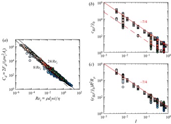
 $\eta$. Interestingly, as detailed in Appendix C, our drag model can be recast into an
 $I^{-7/4}$ form, and the resulting scaling is slightly more general than that of Bancroft & Johnson (Reference Bancroft and Johnson2021) as it captures the results for the full range of
 $I$,
 $R$ and
 $R_\rho$.
Finally, our results for the drag force using uniform shear to avoid gradient-induced segregation forces are quantitatively consistent with other work using uniform shear (Liu & McCarthy Reference Liu and McCarthy2017; Duan et al. Reference Duan, Umbanhowar, Ottino and Lueptow2020; Bancroft & Johnson Reference Bancroft and Johnson2021). However, the dependence of  $c$ on
 $I$ for
 $R=1$ (
 $1.45< c<1.75$; figure 7a) only agrees qualitatively with studies using inclined chute flow (Tripathi & Khakhar Reference Tripathi and Khakhar2011, Reference Tripathi and Khakhar2013), where
 $c$ increases from
 $2.57$ to
 $3.67$ as the chute slope is increased from
 $22^\circ$ to
 $29^\circ$ (for
 $R=1$). Our preliminary investigation attributes this discrepancy to an interesting effect related to the direction of the external forcing: in uniform shear flows (no gravity) the external force
 $F_{ext}$ is applied perpendicular to the shear direction (figure 1a), while in inclined chute flows the external force (due to gravity) has a component parallel to the shear flow. Indeed, when we tilt
 $F_{ext}$ towards the positive
 $x$-direction, a greater drag coefficient is measured in the
 $z$-direction (data not shown). We speculate that the drag enhancing effect is related to a lift force (in
 $z$) on the intruder particle as the
 $x$-component of
 $F_{ext}$ induces a velocity difference between the intruder and the mean flow in the
 $x$-direction (Ding et al. Reference Ding, Gravish and Goldman2011; van der Vaart et al. Reference van der Vaart, van Schrojenstein Lantman, Weinhart, Luding, Ancey and Thornton2018; van Schrojenstein Lantman Reference van Schrojenstein Lantman2019; van Schrojenstein Lantman et al. Reference van Schrojenstein Lantman, van der Vaart, Luding and Thornton2021). Further investigation is warranted to address this issue more conclusively but is beyond the scope of this work.
4.2. Implications for gravity-driven segregation
An important application of the results obtained in this paper is in models of mixing and segregation, for which a central question is how to connect the segregation velocity (or flux) with flow conditions (Umbanhowar et al. Reference Umbanhowar, Lueptow and Ottino2019). In the single intruder limit considered here, this can be done by resolving the segregation velocity based on the equation of motion of the intruder particle, provided that all relevant forces acting on the intruder are known. In a more typical granular flow where gravity is present, the forces acting on the intruder include the intruder weight, the segregation driving force  $F_{seg}$ (Guillard et al. Reference Guillard, Forterre and Pouliquen2016; van der Vaart et al. Reference van der Vaart, van Schrojenstein Lantman, Weinhart, Luding, Ancey and Thornton2018; Jing et al. Reference Jing, Ottino, Lueptow and Umbanhowar2021), and the net resistive drag force
 $F_d$, noting that both
 $F_{seg}$ and
 $F_d$ originate from particle contacts and the net contact force on the intruder is not necessarily aligned with the shear, e.g. in inclined-plane flows (Tripathi & Khakhar Reference Tripathi and Khakhar2011; Jing, Kwok & Leung Reference Jing, Kwok and Leung2017; van Schrojenstein Lantman Reference van Schrojenstein Lantman2019; van Schrojenstein Lantman et al. Reference van Schrojenstein Lantman, van der Vaart, Luding and Thornton2021). For simplicity, we consider a horizontal shear flow in the
 $x$-direction where gravity is in the negative
 $z$-direction, and focus only on the vertical motion of the intruder relative to the bed; that is, along the
 $z$-direction,
 \begin{equation} m_i \frac{\partial w_i}{\partial t} ={-} m_i g + F_{seg} + F_d, \end{equation}
where  $m_i=({\rm \pi} /6)\rho _i d_i^3$ is the intruder mass,
 $g$ is the gravitational acceleration and
 $F_d=-c{\rm \pi} \eta d_i w_i$ is the viscous drag force established here (note that the signs of
 $F_d$ and
 $w_i$ have been omitted up to this point but are now specified for clarity). As is evident from (4.1), the segregation propensity (rising and sinking) of the intruder particle in the
 $z$-direction depends only on the imbalance between
 $m_i g$ and
 $F_{seg}$ (Jing et al. Reference Jing, Ottino, Lueptow and Umbanhowar2020), while the intruder velocity
 $w_i$ depends further on the net resistive drag force
 $F_d$.
Generally, the segregation force  $F_{seg}$ consists of two additive terms related to pressure gradients and shear gradients along the
 $z$-direction in the flow (Guillard et al. Reference Guillard, Forterre and Pouliquen2016; Jing et al. Reference Jing, Ottino, Lueptow and Umbanhowar2021). To further simplify the problem, we consider a uniform shear flow in the presence of gravity (which is possible using the stabilizing force approach as detailed in Appendix A), where
 $F_{seg}$ is well described by a size-ratio-dependent buoyancy force (Jing et al. Reference Jing, Ottino, Lueptow and Umbanhowar2020), i.e.
 $F_{seg}=f\phi \rho gV_i$. Here,
 $f=f(R)$ is a dimensionless empirical function independent of
 $I$ (Jing et al. Reference Jing, Ottino, Lueptow and Umbanhowar2020) and is reproduced as the dotted curve in figure 8(a),
 $\phi \rho$ represents the bulk density of the granular flow and
 $V_i=({\rm \pi} /6)d_i^3$ is the intruder volume. Assuming steady-state intruder migration (
 $\partial w_i/\partial t = 0$) in the
 $z$-direction, which is typical for intruders in dense granular flows (Staron Reference Staron2018), and substituting the force models above into (4.1) leads to an expression for the intruder velocity,
 \begin{equation} w_i={-}\frac{(\rho_i-f\phi\rho)gd_i^2}{6c\eta}, \end{equation}
which is similar to the terminal velocity of a sphere in a viscous fluid (i.e, if  $f=1$ and
 $c=3$), but with modified buoyancy and drag terms, i.e.
 $f=f(R)$ and
 $c=c(I,R,R_\rho )$, to account for granular effects. Note that
 $w_i$ is negative if
 $\rho _i>f\phi \rho$ (i.e. the intruder sinks) and is positive if
 $\rho _i< f\phi \rho$ (i.e. the intruder rises), keeping in mind that the negative sign for
 $w_i$ due to the downward applied
 $F_{ext}$ has been omitted in the plots throughout this paper. The previously known effects of the (local) pressure (
 $P$) and shear rate (
 $\dot \gamma$) on the segregation velocity (Fry et al. Reference Fry, Umbanhowar, Ottino and Lueptow2018; Trewhela, Ancey & Gray Reference Trewhela, Ancey and Gray2021) are captured in (4.2) by the (local) effective viscosity,
 $\eta =\mu (I)P/\dot \gamma$, although
 $c$ also depends on
 $I$ (figure 7). In particular, the form of our segregation velocity expression (4.2), after substituting in the expression for
 $\eta$, resembles a recent experimental scaling law for the intruder velocity in cyclic shear (Trewhela et al. Reference Trewhela, Ancey and Gray2021),
 $w_i \propto \mathcal {F}(R)\rho g\dot \gamma d^2/(\mathcal {C}\rho g d+P)$, where
 $\mathcal {F}(R)$ and
 $\mathcal {C}$ are empirical fits, which is based on velocity measurements and dimensional analysis.
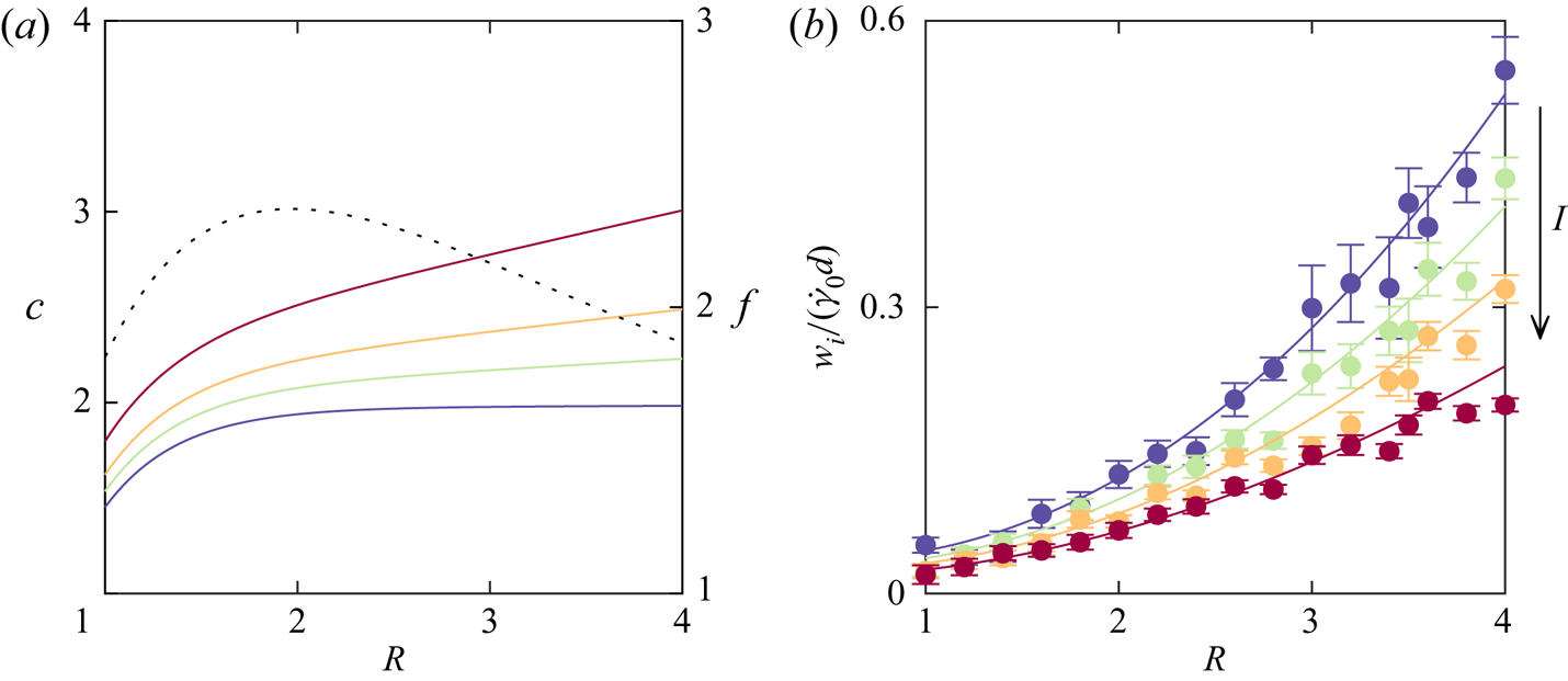
(a) Solid curves (left-hand axis) are  $c=c(R)$ for
 $R_\rho =4$ and
 $I_{loc}=\{0.005,0.1,0.2,0.4\}$ (see text) according to the empirical fit (3.2); colours from blue to red indicate increasing
 $I$. The dotted curve (right-hand axis) is
 $f(R)=[1-1.43\exp (-R/0.92)][1+3.55\exp (-R/2.94)]$, which is independent of
 $I$ (Jing et al. Reference Jing, Ottino, Lueptow and Umbanhowar2020). (b) Simulation results of
 $w_i/(\dot \gamma _0d)$ versus
 $R$ (circles) for gravity-induced sedimentation of heavy intruders in uniform shear flows (see text) and the corresponding predictions (curves) of model (4.2); colours from blue to red match those in (a). Error bars in (b) represent the standard error of
 $w_i$.

To test (4.2) for its applicability to gravity-driven segregation of intruder particles, we run additional simulations with the same set-up as figure 1(a), except with  $g=9.81$ m s
 $^{-2}$ in the vertical direction and
 $F_{ext}=0$, allowing heavy intruders (with a fixed density ratio of
 $R_\rho =4$ and various
 $R$ from
 $1$ to
 $4$) to sink under gravity through the flow with four sets of flow conditions (
 $P_0=1000$ Pa and
 $\dot \gamma _0=\{1,20,40,80\}$ s
 $^{-1}$). In each simulation, a constant shear rate
 $\dot \gamma _0$ is maintained due to the stabilizing forces (Appendix A), but the stress fields are no longer homogeneous as gravity introduces a constant vertical pressure gradient. Therefore, instead of using system parameters
 $P_0$ and
 $\dot \gamma _0$, we measure the average values of
 $\phi$,
 $\mu$,
 $P$ and
 $\dot \gamma$ (as well as the corresponding mean intruder velocity
 $w_i$) over a
 $10d$-thick layer in the middle of the flow to compute the local inertial number
 $I_{loc}=\dot \gamma d/\sqrt {P/\rho }$ and viscosity
 $\eta =\mu P/\dot \gamma$; note that these local measurements are undisturbed by the presence of intruders due to spatial smoothing and temporal averaging (Jing et al. Reference Jing, Ottino, Lueptow and Umbanhowar2021). The simulation results for
 $w_i$ versus
 $R$ for each set of flow conditions (
 $I_{loc}=\{0.005,0.1,0.2,0.4\}$, respectively) are presented as symbols (from blue to red colours) in figure 8(b). Note that
 $w_i$ is normalized by
 $\dot \gamma _0 d$, a constant characteristic velocity for each data series. Interestingly, the values of
 $w_i/(\dot \gamma _0 d)$ (varying from
 $0.01$ to
 $0.3$) for
 $R\lesssim 3$ are quantitatively consistent with previous segregation velocity results for size-bidisperse and density-bidisperse mixtures in heap flows (Schlick et al. Reference Schlick, Fan, Isner, Umbanhowar, Ottino and Lueptow2015; Xiao et al. Reference Xiao, Umbanhowar, Ottino and Lueptow2016; Duan et al. Reference Duan, Umbanhowar, Ottino and Lueptow2021), confirming the connection between
 $w_i$ determined from the force balance on a single intruder (4.2) and the segregation velocity model determined in particle mixtures to predict segregation in granular flows (Umbanhowar et al. Reference Umbanhowar, Lueptow and Ottino2019).
The predictions of (4.2) are obtained by first calculating  $c=c(R)$ for each
 $I$ (solid curves with blue to red colours in figure 8a) for fixed
 $R_\rho =4$ according to (3.2) and then calculating the corresponding
 $w_i(R)$ (solid curves in figure 8b) according to (4.2). Good agreement between the predictions and the simulation results is obtained for all data series in figure 8(b), which confirms the applicability of our segregation velocity model (4.2) to gravity-driven segregation in uniform shear, at least for the density ratio,
 $R_\rho =4$, that we consider. For a wider range of
 $R_\rho$, a rich variety of rising and sinking behaviours can occur depending on the combination of
 $R$ and
 $R_\rho$ (Félix & Thomas Reference Félix and Thomas2004; Jing et al. Reference Jing, Ottino, Lueptow and Umbanhowar2020), but this is not examined further in this work. Moreover, we highlight that the
 $w_i(R)$ curves in figure 8(b) exhibit a monotonic trend similar to the size ratio dependence of the segregation velocity in previous cyclic shear (Trewhela et al. Reference Trewhela, Ancey and Gray2021) and bedload transport studies (Chassagne et al. Reference Chassagne, Maurin, Chauchat, Gray and Frey2020; Rousseau et al. Reference Rousseau, Chassagne, Chauchat, Maurin and Frey2021), which demonstrates the potential relevance of our model to these different systems. It is also evident from figure 8(a) that, although the strength of the segregation force,
 $f(R)$, has a peak at
 $R\approx 2$ (Guillard et al. Reference Guillard, Forterre and Pouliquen2016; van der Vaart et al. Reference van der Vaart, van Schrojenstein Lantman, Weinhart, Luding, Ancey and Thornton2018; Jing et al. Reference Jing, Ottino, Lueptow and Umbanhowar2020; Liu & Müller Reference Liu and Müller2021),
 $w_i$ increases monotonically with
 $R$ due to the combined effects of
 $f(R)$ and
 $c(R)$ in (4.2). Finally, the increasing trend of
 $w_i(R)$ in figure 8(b) is based on results in the single intruder limit, whereas a somewhat different trend of the segregation velocity in size-bidisperse mixtures has been found, which increases with
 $R$ but plateaus for
 $R\gtrsim 3$ (Schlick et al. Reference Schlick, Fan, Isner, Umbanhowar, Ottino and Lueptow2015). This likely indicates the influence of an additional segregation mechanism (free sifting) in mixtures with relatively large size ratios (
 $R\gtrsim 3$), whereby fine particles can more readily percolate through the matrix of coarse particles.
5. Conclusions
In this paper, we use extensive DEM simulations to explore the net resistive drag force on a spherical intruder in uniformly sheared dense granular flows in the absence of gravity. The simulations encompass a parameter space that is broader than explored previously, including drag forces  $0.01\leqslant F_d/(P_0d_i^2)\leqslant 100$, inertial numbers
 $10^{-3}\lesssim I \lesssim 1$, intruder size ratios
 $0.6\leqslant R \leqslant 5$ and intruder density ratios
 $1\leqslant R_\rho \leqslant 20$. Three regimes of drag behaviour over the space defined by the dimensionless drag force
 $F_d/(P_0d_i^2)$ and the dimensionless inertial number
 $I$ are observed (figure 3c,e), including a fluctuation-dominated regime for small
 $F_d/(P_0d_i^2)$ where it is difficult to accurately measure
 $w_i$ in our simulation geometry, a viscous-like regime for intermediate
 $F_d/(P_0d_i^2)$ where
 $F_d \propto w_i$, and an inertia-like regime for large
 $F_d/(P_0d_i^2)$ where cavity formation occurs and the scaling relation transitions towards
 $F_d \propto w_i^2$; the transitional behaviour between the viscous and inertial scaling depends on
 $I$. Despite the variety of intruder dynamics displayed in these drag regimes, the viscous-like scaling remains relevant even when cavity formation occurs for a range of intermediate
 $I$ due to the transition from viscous to inertial behaviour. The viscous-like scaling may also be relevant in the fluctuation-dominated regime, although it is difficult to assess using our approach here due to the large fluctuations in the motion of intruder particles. Nevertheless, as a result of the dominance of the
 $F_d \propto w_i$ scaling, nearly all simulation results collapse onto a master curve, which can be described by a Stokesian drag model,
 $C_d=8c/Re_i$, or
 $F_d=c{\rm \pi} \eta d_i w_i$ (3.1), for
 $Re_i$ spanning over five orders of magnitude (
 $10^{-5}\lesssim Re_i \lesssim 1$), as is summarized in figure 9, which includes all data from figures 4, 6 and 7. Even within the remarkable collapse of the data in figure 9, the value for the drag prefactor
 $c=c(I,R,R_\rho )$, which varies approximately from
 $1$ to
 $3$, can be described by an empirical expression (3.2).
Summary of  $C_d$ versus
 $Re_i$ data for all (
 $I$,
 $R$,
 $R_\rho$) conditions explored in this paper, including over
 $1000$ simulations with
 $0.01\leqslant F_d/(P_0d_i^2)\leqslant 100$,
 $10^{-3}\lesssim I \lesssim 1$,
 $0.6\leqslant R \leqslant 5$ and
 $1\leqslant R_\rho \leqslant 20$. Symbol colours match those in figure 7, and the solid, dashed, dotted and dot–dash model curves are identical to those in figures 4 and 6.

The Stokesian drag model (3.1) developed here indicates a striking similarity between intruder drag in a granular flow and drag on a sphere in a viscous fluid. This also leads to a terminal velocity-like formulation for the intruder velocity (4.2) by combining the Stokesian drag model with a previously established Archimedean segregation force model for uniform shear flows (Jing et al. Reference Jing, Ottino, Lueptow and Umbanhowar2020). As discussed in § 4.2, this ‘granular terminal velocity’ captures the dependence of the intruder segregation velocity on the flow conditions and the particle size and density ratios, matching our simulation results of gravity-driven segregation of heavy intruders in uniform shear, as well as resembling some aspects of previous segregation studies using heap flow (Schlick et al. Reference Schlick, Fan, Isner, Umbanhowar, Ottino and Lueptow2015; Xiao et al. Reference Xiao, Umbanhowar, Ottino and Lueptow2016; Duan et al. Reference Duan, Umbanhowar, Ottino and Lueptow2021), cyclic shear (Trewhela et al. Reference Trewhela, Ancey and Gray2021) and bedload transport (Rousseau et al. Reference Rousseau, Chassagne, Chauchat, Maurin and Frey2021). Hence, although our drag model is developed in an idealized uniform shear flow in the absence of gravity for an isolated intruder, it appears to be relevant to more complicated granular shear flows where stress gradients and kinematics gradients exist. Indeed, our preliminary tests indicate that the drag coefficient is insensitive to the presence of gravity or an arbitrary shear rate gradient in the flow, using the velocity profile control approach of Jing et al. (Reference Jing, Ottino, Lueptow and Umbanhowar2021). The insensitivity of the drag force to gradients in the flow is not surprising and is analogous to the drag in a viscous fluid. Nevertheless, future work should further confirm or extend the applicability of our model (3.1) in different granular flow configurations.
Despite the simplicity of our drag model and its effectiveness over a broad range of conditions, the model is not the complete answer and many research directions remain for developing a fuller understanding of drag in granular flows. First, it would be interesting to further explore the directionality of the intruder drag following the third discussion point in § 4.1. Although we focus on the net intruder force and velocity in the  $z$-direction, the streamwise (
 $x$) intruder velocity relative to the mean flow velocity may also affect the measured drag force by inducing lift effects in the
 $z$-direction (Ding et al. Reference Ding, Gravish and Goldman2011; van der Vaart et al. Reference van der Vaart, van Schrojenstein Lantman, Weinhart, Luding, Ancey and Thornton2018). The lift is likely to be more important if the net drag force has an angle with respect to the
 $z$-direction (see § 4.1) or for a very heavy intruder which has significant inertia in the flow direction. Indeed, it may be useful to consider the intruder drag in both streamwise and depthwise directions as a coupled process, because typically the orientation of the contact forces on intruder particles is anisotropic (see, e.g. figure 1a inset) with a principal contact orientation unaligned with the shear direction (Azéma & Radjaï Reference Azéma and Radjaï2014; Jing et al. Reference Jing, Kwok and Leung2017; van Schrojenstein Lantman Reference van Schrojenstein Lantman2019; van Schrojenstein Lantman et al. Reference van Schrojenstein Lantman, van der Vaart, Luding and Thornton2021). Second, while we focus on granular flows well above yielding (
 $I>10^{-3}$), non-local effects can also play a role in drag if
 $I$ is further decreased towards the creeping flow regime (Candelier & Dauchot Reference Candelier and Dauchot2009; Nichol et al. Reference Nichol, Zanin, Bastien, Wandersman and van Hecke2010; Reddy et al. Reference Reddy, Forterre and Pouliquen2011; Zheng et al. Reference Zheng, Wang, Barés and Behringer2018). In fact, the fluctuation-dominated regime in figure 2(a), which is a consequence of intermittency in the intruder dynamics, may be related to non-locality in granular materials (Kamrin Reference Kamrin2019). Finally, from a practical standpoint, it is necessary to extend the current drag and segregation velocity models from the single intruder limit towards mixtures with finite particle concentrations, perhaps in a way similar to our recent work on the segregation driving force (Duan et al. Reference Duan, Jing, Umbanhowar, Ottino and Lueptow2022), thereby developing a more general framework for continuum modelling of granular segregation (Bancroft & Johnson Reference Bancroft and Johnson2021; Rousseau et al. Reference Rousseau, Chassagne, Chauchat, Maurin and Frey2021; Tripathi et al. Reference Tripathi, Kumar, Nema and Khakhar2021; Duan et al. Reference Duan, Jing, Umbanhowar, Ottino and Lueptow2022).
Supplementary movies
Supplementary movies are available at https://doi.org/10.1017/jfm.2022.706.
Acknowledgements
We thank Y. Fan, J. Hecht and Y. Duan for valuable discussions. The research is facilitated in part by the computational resources and staff contributions provided by the Quest high performance computing facility at Northwestern University, which is jointly supported by the Office of the Provost, the Office for Research and Northwestern University Information Technology.
Funding
This material is based upon work supported by the National Science Foundation under grant no. CBET-1929265.
Declaration of interests
The authors report no conflict of interest.
Appendix A. Uniform shear using force feedback
In this work, simple shear (figure 1a) is used to avoid segregation effects on the intruder that can occur due to pressure and shear gradients (Jing et al. Reference Jing, Ottino, Lueptow and Umbanhowar2021). However, uniform flow fields do not necessarily result for all flow conditions when simply translating the upper wall due to shear localization near the walls, especially for relatively thick flows (reaching approximately  $35d$ in thickness here). To ensure uniform shear along the flow depth, we apply a small streamwise stabilizing force to each DEM particle (except the intruder) at each time step,
 \begin{equation} F_s=K_s[u(z_p)-u_p], \end{equation}
where  $z_p$ and
 $u_p$ are the instantaneous particle position and velocity, respectively, and
 $u(z)=\dot \gamma _0 z$ is the desired uniform shear velocity profile. This velocity control approach has been adopted widely to study granular rheology (Lerner et al. Reference Lerner, Düring and Wyart2012; Clark et al. Reference Clark, Thompson, Shattuck, Ouellette and O'Hern2018) and segregation (Fry et al. Reference Fry, Umbanhowar, Ottino and Lueptow2018; Duan et al. Reference Duan, Umbanhowar, Ottino and Lueptow2020) in uniform shear flows, but it can also be applied to explore arbitrarily non-uniform shear (Saitoh & Tighe Reference Saitoh and Tighe2019; Jing et al. Reference Jing, Ottino, Lueptow and Umbanhowar2021). The parameter
 $K_s$ determines how much the stabilizing force affects the flow kinematics; it should be small enough to not alter the granular flow rheology and large enough to ensure satisfactory linear velocity profiles. However, the value of
 $K_s$ has previously been determined in an ad hoc manner, depending on the flow conditions (Fry et al. Reference Fry, Umbanhowar, Ottino and Lueptow2018).
Here, we use a dimensional analysis to shed light on the appropriate range of  $K_s$. The applied stabilizing forces on an assembly of particles can be viewed as an external force with strength proportional to the difference between the particle velocity and the desired velocity profile, and the latter is approximately the same as the mean steady-state flow velocity if the velocity control is effective. Therefore, at steady state, the mean stabilizing force is proportional to the velocity fluctuation of the flow; that is,
 \begin{equation} \langle F_s \rangle \propto K_s\sqrt{T}, \end{equation}
where  $\langle {\cdot } \rangle$ denotes ensemble average,
 $T=(\delta {u^2}+\delta {v^2}+\delta {w^2})/3$ is the granular temperature of the particle assembly (Weinhart et al. Reference Weinhart, Hartkamp, Thornton and Luding2013) and
 $(\delta u,\delta v,\delta w)$ are the
 $(x,y,z)$-components of the velocity fluctuation. For dense granular flows, the velocity fluctuation (or, here, the square root of the granular temperature) follows a general scaling law,
 \begin{equation} \sqrt{T} \propto \dot\gamma_0 d I^\alpha, \end{equation}
where  $\alpha$ is a system-dependent parameter (da Cruz et al. Reference da Cruz, Emam, Prochnow, Roux and Chevoir2005; Kim & Kamrin Reference Kim and Kamrin2020; Bancroft & Johnson Reference Bancroft and Johnson2021; Rognon & Macaulay Reference Rognon and Macaulay2021). Recent DEM simulations (Kim & Kamrin Reference Kim and Kamrin2020; Bancroft & Johnson Reference Bancroft and Johnson2021) suggest
 $\alpha = -0.25$ for three-dimensional uniform shear flows, which approximately matches the slope of our uncontrolled (as well as weakly controlled) flow results in figure 10(a).
Effects of  $\tilde {K}_s$ on (a)
 $\sqrt {T}/(\dot \gamma _0 d)$, (b)
 $\chi /\chi _0$, (c)
 $\mu$ and (d)
 $\phi$ versus
 $I$. Filled circles with light to dark shading are velocity-controlled flows with
 $\tilde {K}_s=\{0.01,0.05,0.1,0.5,1\}$, while red crosses are uncontrolled, simple shear flows (
 $\tilde {K}_s=0$). The dotted lines in (a,b) indicate, respectively, a slope of
 $-0.25$ and a perfect linear velocity profile (
 $\chi /\chi _0=1$), while the dotted curves in (c,d) are empirical fits identical to the curves in figure 1(b,c). The flow properties
 $T$,
 $\mu$, and
 $\phi$ are averaged in a
 $10d$-thick layer in the middle of the flow, while the shape factor
 $\chi$ is computed considering the entire velocity profile between the lower and upper bounding walls.

Substituting (A3) into (A2) and dividing both sides of (A2) by a force scale  $P_0d^2$ results in
 \begin{equation} \frac{\langle F_s \rangle}{P_0d^2} \propto \frac{K_s\dot\gamma_0 I^\alpha}{P_0d}, \end{equation}
which indicates that the dimensionless stabilizing force,  $\tilde {F}_s=\langle F_s \rangle /(P_0d^2)$, is controlled by a dimensionless parameter
 $\tilde {K}_s=K_s\dot \gamma _0 I^\alpha /(P_0d)$ and that
 $\tilde {F}_s$ characterizes the relative significance of the applied stabilizing force with respect to the mean contact force in the flow resulting from the applied pressure. Based on this understanding, we systematically vary
 $\tilde {K}_s$ as
 $\{0.01,0.05,0.1,0.5,1\}$ (from light to dark filled symbols in figure 10) for
 $10^{-3}\lesssim I \lesssim 1$ (same flow conditions as in figure 1) to determine the appropriate range for
 $\tilde {K}_s$. From figure 10(a), it is evident that values of
 $\tilde {K}_s$ that are too small produce similar results to uncontrolled flow (red crosses in figure 10a), while values of
 $\tilde {K}_s$ that are too large result in deviation from the
 $\alpha =-0.25$ slope, as the velocity fluctuation is over-modulated by
 $\tilde {F}_s$ (mainly in the
 $x$-direction along which
 $\tilde {F}_s$ is applied). For intermediate
 $\tilde {K}_s$, the data match nearly perfectly with the
 $\alpha =-0.25$ slope.
To assess if the velocity profile  $u(z)$ is linear, we define a shape factor
 $\chi =\overline {u^2}/{\bar {u}}^2$ for each flow velocity profile, where the over-bar indicates depth averaging. We then compare
 $\chi$ with a reference value
 $\chi _0=4/3$, which represents a perfectly linear
 $u(z)$, in figure 10(b). The
 $\chi /\chi _0$ results of uncontrolled, simple shear simulations (red crosses) exhibit clear deviations from
 $\chi /\chi _0=1$ (dotted line), indicating non-uniform shear. Likewise,
 $\tilde {K}_s=0.01$ (weakly controlled flow) results in
 $\chi /\chi _0$ slightly less than one, which is expected because too small of a value for
 $\tilde {K}_s$ will not result in the desired linear velocity profile. By contrast, near-perfect uniform shear is achieved for
 $\tilde {K}_s\geqslant 0.05$.
Figures 10(c) and 10(d) show how the choice of  $\tilde {K}_s$ affects the flow rheology in terms of the effective friction
 $\mu$ and packing density
 $\phi$ (measured in a
 $10d$ layer in the middle of the flow). The controlled flows with
 $\tilde {K}_s=\{0.05,0.1,0.5\}$ are not significantly affected, while smaller and larger values of
 $\tilde {K}_s$ lead to slight deviations from the typical rheology. Nevertheless, we have verified that the deviation does not affect the drag and segregation results in the
 $z$-direction, because the velocity control is applied only in the
 $x$-direction. Based on this assessment, we use
 $\tilde {K}_s=0.1$ in our main simulations for the full range of
 $I$ and note that increasing or decreasing
 $\tilde {K}_s$ by an order of magnitude does not alter the results.
Appendix B. Empirical fit of the $c=c(I,R,R_\rho )$ relation

It would be ideal to have a functional form for  $c=c(I,R,R_\rho )$ to complement the Stokes-like drag model (3.1), but a theory-based approach is unclear due to the complex geometric and mass effects typical of dense granular flows (Liu & Müller Reference Liu and Müller2021). Here, we propose an empirical model for
 $c=c(I,R,R_\rho )$ by exploiting the self-similar shape of the different data series in figure 7(b) and the linear correlations in figure 7(a,c). We first use an exponential function combined with a linear term, inspired by the shape of a regularized Bingham viscoplastic constitutive model (Papanastasiou & Boudouvis Reference Papanastasiou and Boudouvis1997), to fit the
 $I=0.008$ data in figure 7(b),
 \begin{equation} c|_{R_\rho=1,I=0.008}=[k_1-k_2\exp({-}k_3R)]+k_4R, \end{equation}
where  $k_1=2$,
 $k_2=7$,
 $k_3=2.6$ and
 $k_4=0.005$ are fitting parameters specific to
 $I=0.008$. Then, we fix
 $k_1$,
 $k_2$ and
 $k_3$ (for simplicity) and fit (B1) to other data series in figure 7(b) to obtain
 $k_4$ for different
 $I$, which leads to
 \begin{equation} k_4=s_1I, \end{equation}
where  $s_1=0.57$. Note that
 $k_4$, which depends linearly on
 $I$, is the slope of the asymptotic line for each curve in figure 7(b). This yields a function for
 $c$ that depends on
 $I$,
 \begin{equation} c|_{R_\rho=1}=[k_1-k_2\exp({-}k_3R)]+s_1IR, \end{equation}
which matches the  $R=1$ and
 $R=4$ data (solid lines in figure 7a).
Finally, we assume that the effects of  $R$ and
 $R_\rho$ are additive and that
 $c$ depends linearly on
 $R_\rho$ with a slope that is different for different
 $I$ (see figure 7c), i.e.
 \begin{equation} c=[k_1-k_2\exp({-}k_3R)]+s_1IR+s_2I(R_\rho-1), \end{equation}
where  $s_2=0.1$ is obtained by fitting (B4) to each data series in figure 7(c). Note that (B4) is identical to (3.2) in the main text and that (B4) reduces to (B3) when
 $R_\rho =1$.
Figure 7(a–c) show that our empirical model (B4) (solid curves) matches each data series (symbols with colour matching the corresponding curves), and, alternatively, the agreement is demonstrated in figure 7(d) by plotting the results of  $c$ from figure 7(a–c) against the values for
 $c$ using (B4) for all simulation conditions of (
 $I,R,R_\rho$). Moreover, the additivity assumption in (B4) is confirmed in figure 7(d) by simulation results of simultaneously varied intruder size and density ratios, i.e.
 $(R,R_\rho )=(2,5)$ and
 $(R,R_\rho )=(2,10)$, for various inertial numbers (
 $I=\{0.008,0.16,0.32,0.64\}$).
Appendix C. Connections with a previous drag model
Bancroft & Johnson (Reference Bancroft and Johnson2021) developed a drag model using DEM simulations of density-bidisperse mixtures in a shear cell with Lees–Edwards boundary conditions,
 \begin{equation} c_{BJ}=\frac{b_i}{w_i}=\frac{\dot\gamma_0}{\kappa I^{7/4}}, \end{equation}
where  $c_{BJ}$ is a (dimensional) drag coefficient,
 $b_i$ is the bulk acceleration acting on species
 $i$,
 $w_i$ is the induced percolation velocity of species
 $i$, and
 $\kappa =0.17$ is a fitting parameter.
A major difference between (C1) and our approach is that instead of using an effective viscosity  $\eta$ to collapse data, Bancroft & Johnson (Reference Bancroft and Johnson2021) directly correlated
 $c_{BJ}/\dot \gamma _0$ with
 $I$. To test if (C1) is applicable to our data (see figure 11a caption) in the intruder limit, we redefine the intruder acceleration as
 $b_i=F_d/m_i$ and recast the data in figure 11(a) into
 $c_{BJ}/\dot \gamma _0$ versus
 $I$ in figure 11(b). Interestingly, this collapses the data for
 $R=1$, leading to quantitative agreement with the scaling relation (C1) (red solid curve). However, the results of varying
 $R$ and
 $R_\rho$ deviate systematically from (C1) (see, e.g. the red dashed curve for
 $R=4$). Therefore, it appears that the
 $\eta$-based scaling in figure 11(a) collapses the data for varying
 $R$ and
 $R_\rho$ better than the
 $I$-based scaling (C1), although the two approaches produce similar data collapse for
 $R=1$.
(a) Identical to figure 9 except that only the data associated with  $0.1\leqslant F_d/(P_0d_i^2)\leqslant 5$ are included (approximately
 $800$ simulations). (b,c) Data recast from (a), where the solid red curves are described by (C1) and (C3) with
 $\kappa =0.17$ and
 $\kappa '=0.17$, respectively. The dashed red curve in (b) has a slope of
 $-7/4$ and passes approximately through the
 $R=4$ data (grey circles).

Another way to connect the two approaches is through our drag model (3.1). We first substitute  $b_i=F_d/m_i=c{\rm \pi} \eta d_i w_i/[({\rm \pi} /6)\rho _id_i^3]$ into (C1), leading to
 \begin{equation} c_{BJ}=\frac{6c\eta}{\rho_i d_i^2}, \end{equation}
and then, noting that  $\eta =\mu P_0/\dot \gamma _0$ and replacing
 $P_0$ by
 $\rho (\dot \gamma _0 d/I)^2$ based on the definition of
 $I$, we rearrange (C2) into
 \begin{equation} c_{BJ}=\frac{6c\mu \rho(\dot\gamma_0 d/I)^2}{\rho_i d_i^2 \dot\gamma_0}=\frac{\dot\gamma_0}{\kappa'I^{7/4}} \frac{1}{R^2R_\rho}, \end{equation}
where  $\kappa '=I^{1/4}/(6 c \mu )$. The resulting scaling,
 $(c_{BJ}/\dot \gamma _0)R^2R_\rho \propto I^{-7/4}$, collapses all data reasonably well in figure 11(c). Noting that
 $c = c(I, R, R_\rho )$, we have
 $\kappa ' = \kappa '(I,R,R_\rho )$, which explains why the data collapse for varying
 $R$ and
 $R_\rho$ is imperfect in figure 11(c).