2. Experimental details

Experiments were carried out in a closed-circuit wind tunnel with a 2.4 m long square test section ( $0.6~\text{m}\times 0.6~\text{m}$ ). The flow non-uniformity is 0.1 % and the longitudinal turbulence intensity $T_{u}$ is 0.3 % in the test section. See Huang, Zhou & Zhou (Reference Huang, Zhou and Zhou2006) for more details of the tunnel. The experimental set-up is schematically shown in figure 1(a). A flat plate of $2.2~\text{m}\times 0.59~\text{m}\times 0.015~\text{m}$ with a clipper-built leading edge is installed horizontally, 0.088 m above the floor of the test section, as a raised floor to control the boundary layer thickness. Its leading edge is 0.3 m downstream of the exit plane of the tunnel contraction.

The vehicle model was a one-third scale Ahmed body (Ahmed et al. Reference Ahmed, Ramm and Faltin1984). The angle ${\it\varphi}$ of the slanted surface was $25^{\circ }$ , at which the wake is characterized by one pair of strong counter-rotating streamwise vortices. This configuration has been deployed to represent the high-drag regime and rather extensively investigated (e.g. Minguez et al. Reference Minguez, Pasquetti and Serre2008). The test model was placed on the raised floor, resulting in a blockage ratio of approximately 4.1 %. Its front end was 0.3 m, where the boundary layer thickness was approximately 4 mm at a free-stream velocity ( $U_{\infty }$ ) of $8.33~\text{m}~\text{s}^{-1}$ , downstream of the floor leading edge. Figure 1(b) shows the definition of the right-handed Cartesian coordinate system ( $x,y,z$ ), with the origin $o$ at the midpoint of the lower edge of the model vertical base. The model has an overall length of $L=0.348~\text{m}$ , a width of $W=0.13~\text{m}$ and a height of $H=0.096~\text{m}$ , supported by four hollow cylindrical struts of 16.67 mm length and 10 mm diameter. In this paper, a superscript asterisk denotes normalization by $\sqrt{A}~(=0.112~\text{m})$ , e.g. $x^{\ast }=x/\sqrt{A},~y^{\ast }=y/\sqrt{A}$ and $z^{\ast }=z/\sqrt{A}$ .

The higher $T_{u}$ was obtained by deploying a grid upstream of the model. The characteristic dimensions of the grid are $M=40~\text{mm}$ , $W=10~\text{mm}$ and $G=10~\text{mm}$ , with a porosity of 64 % (figure 1 a). The grid was installed at the end of the tunnel contraction section, generating closely uniform and isotropic turbulence (Wang et al. Reference Wang, Zhou, Alam and Yang2014). A calibrated hot-wire probe was used to measure the instantaneous streamwise velocity $U$ and $T_{u}$ . A variation in $T_{u}$ was achieved by changing the distance $S$ from the grid to the model frontal face. The choice of $S$ is based on two considerations, i.e. a suitable $T_{u}$ and the uniformity of $\overline{U}$ , where $U$ was measured at a number of points along the $z$ direction and the overbar denotes time averaging. As shown in figure 2(a), there is a discernible variation in $\overline{U}$ across the flow at $S=13M$ but not so at $S=15M$ . Two turbulent intensity levels, i.e.  $T_{u}=7.8\,\%$ and 0.3 %, of the flow are investigated, obtained in the presence ( $S=15M$ ) and absence of the turbulence generator (grid), respectively (figure 2 b).

Figure 2.

(a) The distribution of $\overline{U}$ at $S/M=13$ and 15. (b) The distribution of $T_{u}$ of removing the grid and at $S/M=15$ .

Single hot wires fixed on a computer-controlled Dantec traverse system were used to measure streamwise fluctuating velocity $u$ to detect the predominant frequencies in the flow (figure 1 a). The sensing element was a tungsten wire of $5~{\rm\mu}\text{m}$ diameter and approximately 1 mm in length. The wire was operated on a constant-temperature circuit (Dantec Streamline) at an overheat ratio of 1.8. The signal from the wire was offset, amplified and low-pass-filtered at a cut-off frequency of 1.0 kHz, and digitized at a sampling frequency $f_{s}$ of 3.0 kHz using a 16-bit analogue-to-digital converter (NI PCI-6143). The sampling duration was 1 min, producing a total of $1.8\times 10^{5}$  data for each record. At least three records were collected for each measurement location. Presumably, flow is symmetric with respect to the plane $y^{\ast }=0$ . As such, the hot-wire measurements were performed only on the side of $y^{\ast }=0$ and covered the regions of $x^{\ast }=-2.33$ to $-0.74$ , $y^{\ast }=0$ to 0.58 and $z^{\ast }=0.91$ to 1.09 above the roof, and $x^{\ast }=-2.33$ to $-0.74$ , $y^{\ast }=0.63$ to 0.81 and $z^{\ast }=0$ to 0.86 over the side surface, with increments of ${\rm\Delta}x^{\ast }=0.53$ and ${\rm\Delta}y^{\ast }={\rm\Delta}z^{\ast }=0.036$ . The measurement ranges were $x^{\ast }=-0.51$ to $0$ , $y^{\ast }=0$ to $0.58$ and $z^{\ast }=0.68$ to $0.86$ over the rear window, with increments of ${\rm\Delta}x^{\ast }=0.17$ and ${\rm\Delta}y^{\ast }={\rm\Delta}z^{\ast }=0.036$ , and $x^{\ast }=0.20$ to $2.20$ , $y^{\ast }=0$ to $0.72$ and $z^{\ast }=0$ to $0.81$ behind the base, with increments of ${\rm\Delta}x^{\ast }=0.20$ and ${\rm\Delta}y^{\ast }={\rm\Delta}z^{\ast }=0.09$ . The total number of measurement points amount to more than 2200. The fast Fourier transform (FFT) algorithm was employed to calculate the power spectral density function, $E_{u}$ , of $u$ or the spectral phase between two simultaneously captured hot-wire signals. The FFT window size $N_{w}$ was 4096. The frequency resolution ${\rm\Delta}f$ in the spectral analysis depends on the sampling frequency and the FFT window size ( ${\rm\Delta}f=f_{s}/N_{W}$ ) and is estimated to be 0.73 Hz, following Zhou et al. (Reference Zhou, Du, Mi and Wang2012). Measurements were conducted at $U_{\infty }=6{-}32~\text{m}~\text{s}^{-1}$ , corresponding to $\mathit{Re}=(0.45{-}2.4)\times 10^{5}$ . The wind speed was measured using a Pitot static tube connected to an electronic micro-manometer (Furness Control Ltd, FC510).

A Dantec standard particle image velocimetry (PIV) system was used to measure flow around the Ahmed model at $\mathit{Re}=0.62\times 10^{5}$ . The flow was seeded by smoke generated from paraffin oil, with particles approximately $1~{\rm\mu}\text{m}$ in diameter. Flow illumination was provided by two New Wave standard pulsed laser sources of 532 nm wavelength, each with a maximum energy output of 120 mJ per pulse. Each laser pulse lasted for $0.01~{\rm\mu}\text{s}$ . Particle images were taken using a charge-coupled device (CCD) camera (HiSense type 4M, double frames, $2048~\text{pixel}\times 2048~\text{pixel}$ ). Synchronization between image taking and flow illumination was provided by the Dantec FlowMap processor (System HUB). PIV measurements were performed in the ( $x,z$ ) plane at $y^{\ast }=0$ (symmetry plane), and the ( $y,z$ ) plane at $x^{\ast }=0.20$ . The PIV images covered an area of $2.1\sqrt{A}\times 2.1\sqrt{A}$ , i.e. $x^{\ast }=-0.6$ to 1.5 and $z^{\ast }=-0.3$ to 1.8, and $y^{\ast }=-1.05$ to 1.05 and $z^{\ast }=-0.3$ to 1.8 for the ( $x,z$ ) and ( $y,z$ ) planes, respectively. The image magnifications in both directions of the plane were identical, ranging from 103 to $113~{\rm\mu}\text{m}~\text{pixel}^{-1}$ . The interval between two successive pulses was $50~{\rm\mu}\text{s}$ for measurements in the ( $x,z$ ) plane, during which fluid particles may travel a distance of $0.42~\text{mm}$ at $U_{\infty }=8.33~\text{m}~\text{s}^{-1}$ . Following Huang et al. (Reference Huang, Zhou and Zhou2006), the laser sheet was made thicker for measurements in the ( $y,z$ ) plane, i.e. 3 mm (cf. $1.0{-}1.5~\text{mm}$ in the ( $x,z$ ) plane) in order to capture the maximum number of seeding particles during each pulse. In processing PIV images, $32\times 32$ interrogation areas were used with a 50 % overlap in each direction, producing $127\times 127$ in-plane velocity vectors and the same number of vorticity data ${\it\omega}_{x}^{\ast }$ or ${\it\omega}_{y}^{\ast }$ . A total of 1200 PIV images were captured in each plane.

Laser-induced fluorescence (LIF) flow visualization was conducted using the same PIV system. Three rows of pinholes, each consisting of 64 circular orifices, 1 mm in diameter and equally separated by 1 mm, were made along parallel lines 7 mm upstream of the upper edge of the rear window, the upper and the lower base edges, respectively (figure 1 c). Smoke generated by an Atomizer Aerosol Generator (TSI 3079) using DEHS oil was pumped through one hollow strut into the cavity in the rear part of the model and released into the flow through the pinholes. Flow images were taken in the ( $x,z$ ) planes at $y^{\ast }=0$ and 0.36 over the rear window and at $y^{\ast }=0$ and 0.45 behind the base, and in the ( $y,z$ ) plane at $x^{\ast }=1.4$ in the wake.

3. Flow structures and predominant frequencies in the wake

The wake is highly complicated. In this section we will present and discuss measurement results separately for the region over the rear window and that behind the vertical base. For clarity, we will first examine the data at one Reynolds number, i.e. $\mathit{Re}=0.62\times 10^{5}$ , in this section and also in § 4 and then move on to discussing the effect of Re in § 5.

3.1. Spanwise unsteady flow structure over the rear window

Let us examine the downstream evolution of $E_{u}$ along $\text{A}_{1}{-}\text{A}_{4}$ in the symmetry plane ( $y^{\ast }=0$ ). A peak in $E_{u}$ (figure 3 a) at $f^{\ast }=\mathit{St}_{r}=0.20$ , where subscript $r$ denotes the region above the rear window, is evident at $\text{A}_{1}$ and $\text{A}_{2}$ near the upper edge of the rear window. This peak remains discernible further downstream at $\text{A}_{3}$ but vanishes at $\text{A}_{4}$ . Minguez et al. (Reference Minguez, Pasquetti and Serre2008) observed numerically at ${\it\varphi}=25^{\circ }$ and $\mathit{Re}=8.9\times 10^{5}$ a predominant peak at $\mathit{St}_{r}=0.314$ in $E_{u}$ at a position near $\text{A}_{1}$ in the symmetry plane over the rear window. Their $\mathit{St}_{r}$ is significantly higher than our measurement (0.20). They observed flow separation at the upper edge of the rear window and then reattachment on the slanted surface, which formed a recirculation bubble. The KH instability occurs in the shear layer above the recirculation bubble, which leads to the rollup of spanwise vortices. They ascribed this $\mathit{St}_{r}$ to thus formed vortices over the rear window. Thacker et al. (Reference Thacker, Aubrun, Leroy and Devinant2010) reported a peak in $E_{u}$ at essentially the same $\mathit{St}_{r}~({\approx}0.20)$ based on hot-wire measurements at $\mathit{Re}=(4.5{-}9.0)\times 10^{5}$ at a position near $\text{A}_{1}$ . They suggested that this unsteadiness was mainly due to the flapping recirculation bubble on the slant. A different view will be proposed presently based on our flow visualization data.

Figure 3.

Power spectral density function $E_{u}$ of the hot-wire signal measured along $\text{A}_{1}{-}\text{A}_{4}~(y^{\ast }=0)$ , $\text{B}_{1}{-}\text{B}_{4}~(y^{\ast }=0.36)$ , $\text{C}_{1}{-}\text{C}_{4}~(y^{\ast }=0.58)$ , respectively, over the slant surface.

A peak occurs at $f^{\ast }=\mathit{St}_{r}=0.20$ in $E_{u}$ for all the measurement locations along $\text{B}_{1}{-}\text{B}_{4}$ in the off-symmetry plane of $y^{\ast }=0.36$ (figure 3 b) and is much more pronounced than that measured along $\text{A}_{1}{-}\text{A}_{4}$ . On the other hand, a relatively sharp peak occurs at $f^{\ast }=\mathit{St}_{r}=0.27$ near the side edge of the rear window ( $\text{C}_{1}{-}\text{C}_{4}$ , figure 3 c), where the C-pillar vortex is expected to occur. One minor peak is also discernible at $f^{\ast }=0.53$ , apparently the second harmonic of $\mathit{St}_{r}=0.27$ . Heft et al. (Reference Heft, Indinger and Adams2011) reported at $\mathit{Re}=9.0\times 10^{5}$ a predominant vortex frequency of $\mathit{St}_{r}\approx 0.3$ near the side edge of the slanted surface based on surface pressure measurements. The deviation, albeit small, is probably due to a large difference in Re, inter alia, between the two investigations.

Figure 4 presents typical photographs captured from flow visualization in the planes of $y^{\ast }=0$ and $y^{\ast }=0.36$ over the rear window. The flow appears to separate at the upper edge of the rear window and then to reattach on the slant surface, forming a very small separation bubble (figure 4 a), as shown in Lienhart & Becker’s (Reference Lienhart and Becker2003) velocity measurements in the symmetry plane above the rear window. The shear layer appears to roll up behind this bubble (figure 4 a,b). Kiya & Sasaki (Reference Kiya and Sasaki1985) observed a similar rollup of the shear layer around a rectangular plate and linked this observation to the periodic enlargement and shrinking of the separation bubble. Thus formed vortices are probably responsible for the peak at $\mathit{St}_{r}=0.20$ in $E_{u}$ (figure 3 a,b). Vortex merging is discernible at $y^{\ast }=0$ , as marked in figure 4(a), which corresponds spatially to the vanishing peak in $E_{u}$ at $\text{A}_{4}$ . Krajnović & Davidson (Reference Krajnović and Davidson2005a ) observed numerically the tilted vortices near the lateral sides of the slant, which tended to move towards the central region and merged with each other as convected downstream. They concluded that such vortex merging led to the hairpin vortices being destroyed with both legs broken.

Figure 4.

Typical photographs of the flow structure over the rear window in the ( $x,z$ ) plane: (a) $y^{\ast }=0$ (the symmetry plane); (b) $y^{\ast }=0.36$ . Flow is left to right.

In view of the strong three-dimensionality of the flow over the rear window, the hot-wire measurements were conducted at various spanwise locations. As illustrated in $E_{u}$ (figure 5) measured along $\text{G}_{1}{-}\text{G}_{6}$ at $x^{\ast }=-0.51$ and $z^{\ast }=0.86$ , $\text{H}_{1}{-}\text{H}_{6}$ at $x^{\ast }=-0.17$ and $z^{\ast }=0.79$ , and $\text{I}_{1}{-}\text{I}_{6}$ at $x^{\ast }=0$ and $z^{\ast }=0.75$ , the same predominant structures are captured, one at $\mathit{St}_{r}=0.27$ near the side edge of the rear window ( $y^{\ast }=0.58$ ) and the other at $\mathit{St}_{r}=0.20$ . The latter is linked to spanwise vortices that occur behind the small separation bubble (figures 3 and 4). Evidently, the vortices occur over $y^{\ast }=0{-}0.36$ . It may be inferred that a quasi-periodic spanwise vortex roll is formed over the rear window, as proposed by Wang et al. (Reference Wang, Zhou, Pin and Chan2013). There is a large variation in $E_{u}$ from $y^{\ast }=0.36$ to $y^{\ast }=0.58$ . It seems plausible that the spanwise vortices are suppressed under the effect of the C-pillar vortex near the side edge of the slant surface. The peak at $\mathit{St}_{r}=0.20$ in $E_{u}$ is most pronounced at $y^{\ast }=0.36$ but becomes weaker and even vanishes when approaching $y^{\ast }=0$ (figures 3 and 5). The spanwise vortices generated near the upper edge of the rear window are tilted, travelling downstream towards the central region of the slanted surface under the effect of the C-pillar vortex that grows downstream in size. The spanwise vortices in the central region are inclined to merge with each other and/or break up as convected downstream (Krajnović & Davidson Reference Krajnović and Davidson2005a ).

Figure 5.

Power spectral density function $E_{u}$ of the hot-wire signal measured along $\text{G}_{1}{-}\text{G}_{6}~(x^{\ast }=-0.51,~z^{\ast }=0.86)$ , $\text{H}_{1}{-}\text{H}_{6}~(x^{\ast }=-0.17,~z^{\ast }=0.79)$ , $\text{I}_{1}{-}\text{I}_{6}$ ( $x^{\ast }=0,~z^{\ast }=0.75$ ), respectively, over the slant surface.

3.2. Longitudinal structure over the rear window

Figure 6 presents typical instantaneous ${\it\omega}_{x}^{\ast }$ contours in the ( $y,z$ ) plane at $x^{\ast }=0.2$ . The two most highly concentrated longitudinal vortices, marked by ‘C’, are the well-known C-pillar vortices. On the other hand, a number of alternately signed ${\it\omega}_{x}^{\ast }$ concentrations show up between the C-pillar vortices, which tend to be aligned in one row near the upper edge of the base, as enclosed by thick broken lines. Shabaka, Mehta & Bradshaw (Reference Shabaka, Mehta and Bradshaw1985) examined the evolution of a single longitudinal vortex embedded in a turbulent boundary layer. Their hot-wire-measured vorticity contours showed that the longitudinal vortex induced vorticity, whose sign was opposite to that of the primary vortex, in the region around the primary vortex. Logdberg, Fransson & Alfredsson (Reference Logdberg, Fransson and Alfredsson2009) investigated the evolution of a pair of longitudinal counter-rotating vortices in a turbulent boundary layer based on flow visualization and hot-wire measurements. They advocated that the vortex-induced vorticity, with an opposite sign to that of the primary vortex on the same side, rolled up into a secondary vortex outboard of the pair of primary vortices. As shown in figure 6, in the vicinity of each C-pillar vortex, there appears one relatively strong ${\it\omega}_{x}^{\ast }$ concentration, whose sign is opposite to that of the C-pillar vortex, with the maximum magnitude of ${\it\omega}_{x}^{\ast }$ reaching 7. In view of the induction effect of the two C-pillar vortices, this vorticity concentration is considered to be induced by the C-pillar vortex. For the same reason, the ${\it\omega}_{x}^{\ast }$ concentrations near the symmetry plane ( $y^{\ast }=0$ ), with their maximum magnitudes reaching 5, are probably induced by those secondary vortices.

Figure 6.

The PIV measurement of instantaneous streamwise vorticity ${\it\omega}_{x}^{\ast }$ contours in the ( $y,z$ ) plane $x^{\ast }=0.20$ . The cutoff level is $\pm 1$ , and the contour increment is $\pm 1$ . The thick broken lines enclose a number of alternately signed ${\it\omega}_{x}^{\ast }$ concentrations formed between the C-pillar vortices.

3.3. Flow structures behind the base

Figure 7 presents $E_{u}$ measured at different heights for a number of downstream stations behind the base in the plane of $y^{\ast }=0$ . At $x^{\ast }=0.2$ , which is within the recirculation bubble (e.g. Wang et al. Reference Wang, Zhou, Pin and Chan2013), $E_{u}$ measured along $\text{K}_{1}{-}\text{K}_{6}$ is characterized by one prominent peak at $f^{\ast }=\mathit{St}_{w}=0.44$ over $z^{\ast }=0{-}0.27$ . This peak is hardly discernible for $z^{\ast }>0.36$ . The spatial location where this peak is detected suggests that the unsteady flow structures associated with this peak may be linked to the recirculation bubbles behind the base. By $x^{\ast }=0.4$ ( $\text{L}_{1}{-}\text{L}_{6}$ ), this peak appears more pronounced and becomes evident for higher $z^{\ast }$ , i.e. at $z^{\ast }=0.36$ , implying that the corresponding unsteady structures grow in strength and move upwards as advected downstream. By $x^{\ast }=0.8$ ( $\text{M}_{1}{-}\text{M}_{6}$ ), this peak can even be seen at $z^{\ast }=0.54$ . The unsteady structures appear fully grown and start to decay at larger $x^{\ast }$ ; the peak in $E_{u}$ at $x^{\ast }=1.4~(\text{N}_{1}{-}\text{N}_{6})$ is appreciably less prominent. The result is consistent with the numerical study by Minguez et al. (Reference Minguez, Pasquetti and Serre2008), who observed at $\mathit{Re}=8.9\times 10^{5}$ a predominant St of 0.49 near $x^{\ast }=0.43$ and $z^{\ast }=0$ . The deviation in their St from our measurement is not unexpected in view of the possible boundary and other differences, besides Re, between the numerical and experimental studies. Based on the surface pressure tap measurements, Vino et al. (Reference Vino, Watkins, Mousley, Watmuff and Prasad2005) observed a single predominant frequency at $\mathit{St}\approx 0.39$ at $y^{\ast }=0$ on the upper ( $z^{\ast }=0.40$ ) and lower ( $z^{\ast }=0.13$ ) vertical base of an Ahmed model ( ${\it\varphi}=30^{\circ }$ , the high-drag configuration, $\mathit{Re}=(4.5{-}7.9)\times 10^{5}$ ), and a spectral phase shift of near ${\rm\pi}$ at this St between the pressure signals simultaneously measured at these two locations, that is, the two signals are out of phase. They thus proposed that the recirculation bubbles behind the vertical base behaved similarly to von Kármán vortex shedding from a two-dimensional bluff body such as a square cylinder. It is worth commenting that the von Kármán vortex street is generated by the alternate separation of shear layers from the two trailing edges of a square cylinder (e.g. Alam, Zhou & Wang Reference Alam, Zhou and Wang2011). However, as shown later, the quasi-periodic structures at $\mathit{St}_{w}=0.44$ result from the alternate emanation of fluid parcels from the upper and lower recirculation bubbles. One minor peak is also discernible at $f^{\ast }=0.88$ , the second harmonic of $\mathit{St}_{w}=0.44$ , at $x^{\ast }=0.4{-}0.8$ for $z^{\ast }\leqslant 0.09$ . This harmonic could not be seen at $x^{\ast }=1.4$ .

Figure 7.

Power spectral density function $E_{u}$ of the hot-wire signal measured along $\text{K}_{1}{-}\text{K}_{6}$ , $\text{L}_{1}{-}\text{L}_{6}$ , $\text{M}_{1}{-}\text{M}_{6}$ , $\text{N}_{1}{-}\text{N}_{6}$ , respectively, at $y^{\ast }=0$ in the wake.

Typical flow structures captured from flow visualization are examined in figure 8 in order to obtain a better picture of how the unsteady structures at $\mathit{St}_{w}=0.44$ are generated. At one instant, one structure is shed towards the ground from the upper recirculation bubble behind the base (figure 8 a); at the other instant, another structure appears popping up from the lower recirculation bubble (figure 8 b). The two distinct flow patterns are also observed from typical instantaneous ${\it\omega}_{y}^{\ast }$ contours measured in the symmetry plane ( $y^{\ast }=0$ ) of the wake, as illustrated in figure 8(c,d). The contours further indicate that the emanated structures, as enclosed by a thick contour, are associated with the concentrated vorticity. The fact that the two emanated structures are never seen to occur simultaneously suggests that the organized structures are produced alternately from the upper and lower recirculation bubbles, which are responsible for the pronounced peak at $\mathit{St}_{w}=0.44$ and its second harmonic in $E_{u}$ (figure 7). This is confirmed by the spectral phase shift ${\it\Phi}_{u_{L_{1}}u_{L_{4}}}$ of near ${\rm\pi}$ , i.e. out of phase, at $\mathit{St}_{w}=0.44$ (figure 9 a) between the hot-wire signals simultaneously obtained at $\text{L}_{1}~(z^{\ast }=0)$ and $\text{L}_{4}~(z^{\ast }=0.27)$ . A similar observation on the spectral phase shift is also made at $x^{\ast }=0.8$ . However, the spectral phase shift ${\it\Phi}_{u_{N_{1}}u_{N_{4}}}$ at $\mathit{St}_{w}=0.44$ between the hot-wire signals simultaneously obtained at $\text{N}_{1}~(z^{\ast }=0)$ and $\text{N}_{4}~(z^{\ast }=0.27)$ is near zero at $x^{\ast }=1.4$ , downstream of the recirculation bubbles (figure 9 b). The observation will be explained later in this section.

Figure 8.

Typical instantaneous flow structure in the symmetry plane ( $y^{\ast }=0$ ) in the wake. (a,b) Flow visualization; the white line is the reflection of the laser light from the floor. (c,d) PIV-measured instantaneous spanwise vorticity ${\it\omega}_{y}^{\ast }$ contours; the cutoff level is $\pm 3$ , and the contour increment is $\pm 2$ .

Figure 9.

Spectral phase between hot-wire signals simultaneously measured at: (a)  $\text{L}_{1}$ and $\text{L}_{4}$ ; (b) $\text{N}_{1}$ and $\text{N}_{4}$ . Please refer to figure 7 for the locations of $\text{L}_{1}$ , $\text{L}_{4}$ , $\text{N}_{1}$ and $\text{N}_{4}$ .

One scenario is proposed for the observed unsteady structures at frequencies $\mathit{St}=0.44$ and 0.88. The organized structures are shed alternately from the upper and lower recirculation bubbles, respectively, at a frequency of $\mathit{St}_{w}=0.44$ , as evidenced by the peak in $E_{u}$ from $z^{\ast }=0$ to 0.36 measured at $x^{\ast }=0.4$ (figure 7) and a phase angle of near ${\rm\pi}$ at $\mathit{St}_{w}=0.44$ in ${\it\Phi}_{u_{L_{1}}u_{L_{4}}}$ (figure 9 a). The structure separated from the upper bubble sweeps towards the ground (figure 8 a,c); on the other hand, the structure from the lower bubble is emanated upwards (figure 8 b,d). Figure 8 indicates that the former structure appears short-lived, compared with the latter. This assertion is also consistent with $E_{u}$ measured over $x^{\ast }=0.4{-}1.4$ (figure 7). A small portion of structures shed from the two bubbles may reach the same level of elevation over $x^{\ast }=0.4{-}0.8$ , as supported by the minor peak at $\mathit{St}=0.88$ in $E_{u}$ from $z^{\ast }=0$ to 0.09 in this $x^{\ast }$ range (figure 7). The structure separated from the upper bubble breaks up and disappears before reaching $x^{\ast }=1.4$ , and the peak shown in $E_{u}$ at $x^{\ast }=1.4$ is essentially the signature of structures emanated from the lower bubble. As such, ${\it\Phi}_{u_{N_{1}}u_{N_{4}}}$ is near zero at $\mathit{St}_{w}=0.44$ (figure 9 b). Vino et al. (Reference Vino, Watkins, Mousley, Watmuff and Prasad2005) measured the turbulence intensity using a pressure probe in the ( $x,z$ ) plane at $y^{\ast }=0$ behind the vertical base of an Ahmed model, and observed that the upper recirculation bubble was stretched downstream towards the ground, on the one hand, and the lower bubble stretched downstream upwards, on the other. They advocated that vortex shedding behind the base was a process of alternating stretching of the upper and lower recirculation bubbles. Our proposed scenario provides an accurate account for the flow physical picture and an explanation for their stretched bubbles.

Since the quasi-periodic structures behind the vertical base of the Ahmed model show up with two distinct flow patterns, it could be insightful to extract these structures and characterize each of the two flow patterns. As illustrated in the instantaneous ${\it\omega}_{y}^{\ast }$ contours (figure 8 c,d), the structures emanated from the upper and lower recirculation bubbles are characterized by relatively strong negative- and positive-vorticity concentrations, respectively. Therefore, we detect the occurrence of quasi-periodic structures based on their strength per unit area $J^{\ast }$ , viz.

(3.1) $$\begin{eqnarray}J^{\ast }=\frac{\displaystyle \iint _{S^{\ast }}{\it\omega}_{y}^{\ast }\,\text{d}s^{\ast }}{S^{\ast }},\end{eqnarray}$$

where $S^{\ast }$ is the area of a rectangular region of $x^{\ast }=0.63$ to $0.85$ and $z^{\ast }=-0.02$ to $0.11$ in the symmetry plane ( $y^{\ast }=0$ ). The threshold for $J^{\ast }$ is set at 2.0 after carefully checking detections against the plots of vorticity contours. Out of a total of 1200, 204 images with $J^{\ast }$ values lower than $-2.0$ are identified with pattern 1, i.e. flow emanation from the upper recirculation bubble, and 216 with $J^{\ast }$ values larger than 2.0 fall into the other flow pattern, or pattern 2. The ensemble averages are made for each pattern based on these detections. The dependence of ${\it\delta}=({\it\beta}_{N}-{\it\beta}_{N-{\rm\Delta}N})/{\it\beta}_{N}$ on $N$ was calculated, where ${\it\beta}$ denotes $\langle U\rangle$ and $\langle W\rangle$ , and subscript $N$ or $N-{\rm\Delta}N$ is the number of images ( ${\rm\Delta}N$ is the increment in $N$ ). In this paper, angular brackets denote quantities ensemble-averaged based on the above described detections. The value of ${\it\delta}$ is estimated at the centre of the rectangular region ( $S^{\ast }$ ) over which $J^{\ast }$ is calculated. It has been found that ${\it\delta}$ converges rapidly, with increasing $N$ , to within $\pm 3\,\%$ at $N\approx 200$ for $\langle U\rangle$ and $\langle W\rangle$ (not shown). Similar results have been obtained at other locations, thus indicating that the ensemble-averaged results from 204 (or 216) images are reasonably representative of flow features for each flow pattern.

The time-averaged sectional streamlines from the 1200 PIV-measured instantaneous images measured at $\mathit{Re}=0.62\times 10^{5}$ may allow us to determine the bubble or recirculation length, which is defined by the maximum longitudinal length of the wake bubble or reverse flow region, where $\overline{U}\leqslant 0$ . The lengths of the upper and lower recirculation bubbles are $0.56\sqrt{A}$ and $0.53\sqrt{A}$ , respectively, estimated from figure 10(a). One saddle point, marked by symbol ‘ $\times$ ’, occurs behind the recirculation bubbles. The ensemble-averaged sectional streamlines (figure 10 b) based on the 204 images identified for pattern 1 exhibit a number of changes from the time-averaged streamlines (figure 10 a).

Figure 10.

(a) Time-averaged sectional streamlines; (b–d) ensemble-averaged sectional streamlines; ( $\overline{b}$ ,  $\overline{c}$ ) ensemble-averaged sectional streamlines viewed in a reference frame convecting at ( $U_{c}^{\ast },W_{c}^{\ast }$ ). Symbol ‘ $\times$ ’ denotes the saddle point. The red-coloured broken line in (b,c) indicates the bubble size, determined from time-averaged streamlines. $\mathit{Re}=0.62\times 10^{5}$ .

Firstly, the streamlines (figure 10 b) display a considerable downsize of the upper recirculation bubble but an expanded lower bubble, as compared with their time-averaged counterpart (figure 10 a). To facilitate data interpretation, the recirculation bubbles and the saddle point, shown in the time-averaged sectional streamlines, are indicated by a broken curve and symbol ‘ $\times$ ’ in red (figure 10 b), respectively. The upper bubble is $0.51\sqrt{A}$ in longitudinal length, appreciably shorter than its time-averaged counterpart, $0.56\sqrt{A}$ (figure 10 a), whereas the lower bubble becomes $0.55\sqrt{A}$ , longer than that ( $0.53\sqrt{A}$ ) in figure 10(a). The saddle point is also shifted, compared with that in figure 10(a). Downstream of the saddle point, one structure separated from the upper recirculation bubble, as highlighted by a thick broken line, is seen to sweep towards the ground. This structure is closely connected to the change in bubble size and saddle point position, which have a significant impact on the base pressure of an Ahmed model. In their numerical simulation on active drag control of an Ahmed model ( ${\it\varphi}=25^{\circ },\mathit{Re}=8.9\times 10^{5}$ ), Wassen & Thiele (Reference Wassen and Thiele2008) deployed streamwise steady blowing along the upper and two side edges of the rear window, and the lower and two side edges of the base. Their calculated time-averaged streamlines in the symmetry plane of the wake showed that both upper and lower recirculation bubbles were considerably enlarged longitudinally under control. Meanwhile, the saddle point behind the bubbles was pushed farther downstream. Accordingly, the time-averaged base pressure increased by 14 %. In his numerical simulation in the wake of an Ahmed model ( ${\it\varphi}=25^{\circ }$ ), Krajnović (Reference Krajnović2014) deployed one array of finite-length circular cylinders, upstream of the upper edge of the rear window, for drag reduction. The lengths of the two bubbles behind the base were elongated, associated with a significant drag reduction by 11.6 %.

Secondly, a vortical structure occurs downstream of the saddle point, as shown in figure 10( $\overline{b}$ ). The structure emanated from the upper bubble is characterized by a relatively strong vorticity concentration of negative sign, as evidenced by the instantaneous ${\it\omega}_{y}^{\ast }$ contours (figure 8 c). This concentration however is hardly recognizable in figure 10(b). This is because a vortex is in general only visible in streamlines when viewed from a reference frame convecting with the same velocity as the vortex centre (e.g. Zhou & Antonia Reference Zhou and Antonia1994). Note that vortices may change in location from one PIV snapshot to another. As such, we screened carefully the 204 PIV snapshots identified as pattern 1 and picked up 31 images whose maximum ${\it\omega}_{y}^{\ast }$ concentrations, associated with the emanated structures, occurred at approximately the same location, i.e.  $(x^{\ast },z^{\ast })=(0.79,0.1)$ . Using the velocity ( $U_{c}^{\ast },W_{c}^{\ast }$ ) at this location as that at which the reference frame is convected, then the velocity components $U_{r}^{\ast }$ and $W_{r}^{\ast }$ of the 31 images are determined by

(3.2) $$\begin{eqnarray}\displaystyle & U_{r}^{\ast }=U^{\ast }-U_{c}^{\ast }, & \displaystyle\end{eqnarray}$$

(3.3) $$\begin{eqnarray}\displaystyle & W_{r}^{\ast }=W^{\ast }-W_{c}^{\ast }. & \displaystyle\end{eqnarray}$$

Ensemble-averaged sectional streamlines (figure 10 $\!\overline{b}$ ) for this group of data then display a different flow topology, as in figure 10(b). Two foci occur at $(x^{\ast },z^{\ast })=(0.4,0.39)$ and (0.79, 0.1), respectively. The former is due to the upper recirculation bubble, whose centre deviates from that in figure 10(b) because of different vortex convection velocities used in the calculation of streamlines, and the latter to the vortical structure emanated from this bubble.

The ensemble-averaged data based on the detections of pattern 2 show considerable differences. The sectional streamlines (figure 10 c) display an upper recirculation bubble significantly larger than the lower bubble. This result, along with that shown in figure 10(b), suggests that the bubble, be it upper or lower, reduces considerably in size as a result of a fluid parcel ejected from it. Furthermore, a change occurs in the position of the saddle point, which is shifted upstream and meanwhile closer to the ground, compared with that shown in figure 10(b) and that in figure 10(a). Behind the saddle point, one structure is seen to rebound downstream from the lower recirculation bubble, as enclosed by a thick broken line. As indicated by the instantaneous ${\it\omega}_{y}^{\ast }$ contours (figure 8 d), this structure is characterized by a relatively strong positive-vorticity concentration. But the streamlines (figure 10 c) do not show the presence of a vortical structure corresponding to this concentration. Similarly to the analysis of pattern 1, we examined the 216 PIV snapshots detected for pattern 2 and selected 39 where the maximum ${\it\omega}_{y}^{\ast }$ concentration of the emanated structure occurs at approximately the same location of $(x^{\ast },z^{\ast })=(0.77,0.02)$ . With the reference frame fixed at this location, we may recalculate the ensemble-averaged sectional streamlines based on the 39 snapshots. As shown in figure 10( $\overline{c}$ ), one focus occurs at $(x^{\ast },z^{\ast })=(0.77,0.02)$ , indicating the structure separated from the lower bubble.

Ensemble averaging has also been performed based on the remaining 780 PIV snapshots, excluding those identified for patterns 1 and 2. The lengths of the upper and lower recirculation bubbles in the ensemble-averaged streamlines are approximately $0.57\sqrt{A}$ and $0.54\sqrt{A}$ (figure 10 d), respectively, nearly the same as those in the time-averaged streamlines (figure 10 a).

In their experimental study on flow around a rectangular plate, Kiya & Sasaki (Reference Kiya and Sasaki1985) found that flow separated from the leading edge and then reattached downstream, forming a separation bubble. This bubble was characterized by periodic enlargement and shrinkage, i.e. bubble pulsation, and the shear layer rolled up behind the bubble, forming vortices. Tafti & Vanka (Reference Tafti and Vanka1991) studied numerically the mechanism causing bubble pulsation and conjectured that the bubble expanded as a result of entrainment of fluid from the free stream, which caused a gradual rise in pressure within the bubble. The bubble eventually burst when its pressure reached a certain level, which was associated with an outward movement of fluid in the spanwise direction and the emanation of vortices downstream from the bubble. Enlightened by these studies, we propose a physical process for the growing and shrinking recirculation bubbles and the alternate emanation of fluid structures from the two bubbles based on the present observations.

Figure 11.

Schematic of the physical process for the pulsation of two recirculation bubbles and the generation of a quasi-periodic flow structure.

The entire process may be divided into four phases, as schematically shown in figure 11.

Figure 12.

Power spectral density function $E_{u}$ of the hot-wire signal measured along $\text{P}_{1}{-}\text{P}_{6}$ , $\text{Q}_{1}{-}\text{Q}_{6}$ , $\text{R}_{1}{-}\text{R}_{6}$ , $\text{S}_{1}{-}\text{S}_{6}$ , respectively, at $y^{\ast }=0.45$ in the wake.

Phase A. The flow separated from the upper edge of the model base is entrained into the upper recirculation bubble, resulting in a gradual increase in pressure within the bubble. When the pressure reaches a certain level, the bubble cannot sustain it any more and then collapses. As a result, a structure is emanated towards the ground from the bubble, accompanied by a substantially reduced size of the bubble, as evident in the ensemble-averaged streamlines of pattern 1 (figure 11 b). Meanwhile, part of the fluid in the upper bubble is transported into the lower bubble, as indicated by instantaneous velocity vectors (not shown), due to a pressure differentiation between the two bubbles.

Phase B. After the collapse of the upper bubble, the flow separated from the lower edge of the model base is entrained into the lower recirculation bubble. As such, the pressure within this bubble rises and then exceeds that of the upper bubble, resulting in the movement of fluid from the lower to the upper bubble.

Phase C. The lower bubble continues its rise in size and pressure until its collapse, associated with a sudden downsize and the emanation of a structure from it, as observed in ensemble-averaged sectional streamlines of pattern 2 (figure 10 c). The transport of fluid from the lower to the upper bubble is also evident in the instantaneous velocity vectors (not shown).

Phase D. The upper bubble gradually expands in size and rises in pressure. Part of its fluid will move into the lower bubble once its pressure is higher. At an adequately high pressure, the bubble bursts, which starts the next cycle of bubble pulsation and alternate emanation of structures.

In order to gain insight into the three-dimensionality of unsteady flow structures, the hot-wire measurements were conducted in the ( $x,z$ ) plane of $y^{\ast }=0.45$ for a number of downstream locations. The $E_{u}$ plot (figure 12) displays no peak at $x^{\ast }=0.2$ over $z^{\ast }=0{-}0.36~(\text{P}_{1}{-}\text{P}_{5})$ . But at $z^{\ast }=0.54~(\text{P}_{6})$ one peak is discernible at $f^{\ast }=\mathit{St}_{s}=0.27$ , where the C-pillar vortex occurs. At $x^{\ast }=0.4$ , a small peak at $\mathit{St}_{w}=0.44$ is identifiable at $\text{Q}_{1}~(z^{\ast }=0)$ near the ground. This peak grows and propagates to higher $z^{\ast }$ with increasing $x^{\ast }$ , as observed in the symmetry plane (figure 7). A comparison between figures 7 and 12 indicates that the unsteady flow structures at $\mathit{St}_{w}=0.44$ are formed initially about the symmetry plane behind the base. With increasing $x^{\ast }$ , they move upwards and grow in both strength and spanwise extent. As shown in figure 13, ${\it\Phi}_{u_{S_{1}}u_{S_{4}}}$ between two hot-wire signals measured at $\text{S}_{1}$ and $\text{S}_{4}$ in the ( $x,z$ ) plane of $y^{\ast }=0.45~(x^{\ast }=1.4)$ is near ${\rm\pi}/2$ at $\mathit{St}_{w}=0.44$ (figure 12). This phase shift, neither near ${\rm\pi}$ nor near zero, is probably due to strong interactions between the C-pillar vortex and the unsteady structure, as indicated by flow visualization in the plane of symmetry (figure 8) and also in the lateral plane, shown below.

Figure 13.

Spectral phase between hot-wire signals simultaneously measured at $\text{S}_{1}$ and $\text{S}_{4}$ . Please refer to figure 12 for the locations of $\text{S}_{1}$ and $\text{S}_{4}$ .

Figure 14.

Typical photographs of the flow structure of the wake (flow is left to right): (a) in the ( $x,z$ ) plane ( $y^{\ast }=0.45$ ); (b) in the ( $y,z$ ) plane ( $x^{\ast }=1.4$ ),  $t=t_{0}$ (arbitrary); (c)  $t=t_{0}+120~{\rm\mu}\text{s}$ . The white line results from the reflection of the laser light from the floor.

Figure 15.

Power spectral density function $E_{u}$ of the hot-wire signal measured along $\text{T}_{1}{-}\text{T}_{6}~(x^{\ast }=0.09,~z^{\ast }=0)$ in the wake.

Figure 14(a) presents a typical photograph of flow visualization captured in the ( $x,z$ ) plane of $y^{\ast }=0.45$ . The wake is characterized by the alternate emanation of fluid structures from the upper and lower recirculation bubbles in the symmetry plane (figure 8 a,b) and exhibits an upward growth in the ( $x,z$ ) plane of $y^{\ast }=0.45$ , merging into the C-pillar vortex that occurs above the upper recirculation bubble (figure 14 a). The result is internally consistent with the fact that the peak at $\mathit{St}_{w}=0.44$ does not show up in $E_{u}$ for $z^{\ast }>0.27$ in the near wake (figure 12), obtained in the same plane. It also conforms to Ahmed et al.’s (Reference Ahmed, Ramm and Faltin1984) observation based on the cross-flow velocity measurement, that is, the C-pillar vortices interact with the upper recirculation bubble between $x^{\ast }=0.24$ and 0.60 and then form one pair of counter-rotating trailing vortices in the wake. Figure 14(b,c) shows photographs from flow visualization in the ( $y,z$ ) plane at $x^{\ast }=1.4$ , which is normal to the mean flow direction. One pair of trailing vortices occurs. By comparing two sequential photographs captured at a time interval of $120~{\rm\mu}\text{s}$ , we may determine that the two vortices are counter-rotating, as shown by the arrows in figure 14(c). There is a downwash flow in the central region near $y^{\ast }=0$ induced by the two counter-rotating vortices, as observed from the measured cross-flow velocity distributions in the plane of $x^{\ast }=1.49$ by Lienhart & Becker (Reference Lienhart and Becker2003). Note that the peak at $\mathit{St}_{w}=0.44$ in $\mathit{E}_{u}$ becomes more pronounced at $x^{\ast }=1.4$ along $\text{S}_{1}{-}\text{S}_{4}$ (figure 12), away from the symmetry plane, than its counterpart along $\text{N}_{1}{-}\text{N}_{4}$ in the symmetry plane (figure 7). The observation agrees with Lienhart & Becker’s (Reference Lienhart and Becker2003) measurement of the turbulent kinetic energy in the ( $y,z$ ) plane of $x^{\ast }=1.49$ , which appeared larger away from the symmetry plane.

Hot-wire measurements were conducted along $\text{T}_{1}{-}\text{T}_{6}~(x^{\ast }=0.09,~z^{\ast }=0)$ behind the lower edge of the vertical base to capture possible quasi-periodic structures generated in the gap between the floor and the model’s underside. The $E_{u}$ plot (figure 15) displays two major peaks. One occurs at $f^{\ast }=\mathit{St}_{l}=2.11$ over $y^{\ast }=0.75{-}0.79$ . Wang et al.’s (Reference Wang, Zhou, Pin and Chan2013) PIV measurements in the ( $y,z$ ) plane of $x^{\ast }=0.2~(\mathit{Re}=6.2\times 10^{4})$ showed one vortex near the lower corner of the Ahmed model ( ${\it\varphi}=25^{\circ }$ ) at $(y^{\ast },z^{\ast })\approx (\pm 0.72,-0.01)$ , which they referred to as the lower vortex. This coincidence in the location of $y^{\ast }$ and $z^{\ast }$ does not necessarily suggest a link between the peak at $\mathit{St}_{l}=2.11$ and the lower vortex. It has been confirmed that the unsteady structures of $\mathit{St}_{l}=2.11$ result from vortex shedding from the cylindrical struts located at $x^{\ast }=-2.52$ and $y^{\ast }=\pm 0.49$ between the model underside and the floor, which will be discussed in § 4. The other peak occurs at $f^{\ast }=\mathit{St}_{g}=1.76$ over $y^{\ast }=0.36{-}0.65$ , corresponding spatially to the gap vortex identified by Wang et al. (Reference Wang, Zhou, Pin and Chan2013). Note that this $\mathit{St}_{g}$ corresponds to a dimensionless frequency $\mathit{St}_{D}\approx 0.16$ based on $U_{\infty }$ and the diameter $D$ of the cylindrical strut between the model underside and floor, which is close to the Strouhal number, 0.20, in a circular cylinder wake. The discrepancy is probably due to the effect of the boundary layer in the gap, which reduces the actual fluid speed and hence $\mathit{St}_{D}$ (e.g. Krajnović & Davidson Reference Krajnović and Davidson2005b ; Wang, Zhou & Mi Reference Wang, Zhou and Mi2012). It may be inferred that the peak at $\mathit{St}_{g}=1.76$ is probably associated with the gap vortices generated by the struts located at $x^{\ast }=-1.11$ and $y^{\ast }=\pm 0.49$ .

3.4. The spatial extent of identified unsteady structures

Five distinct vortex frequencies are now identified over the rear window and behind the vertical base, i.e. $\mathit{St}_{r}$ , $\mathit{St}_{s}$ , $\mathit{St}_{w}$ , $\mathit{St}_{g}$ and $\mathit{St}_{l}$ . The locations where they are detected in the ( $y,z$ ) plane vary for different downstream stations. Figure 16 presents their spatial distributions in the ( $y,z$ ) plane at $x^{\ast }=0.2$ , 0.4, 0.8, 1.6 and 2.2. The Strouhal number $\mathit{St}_{i}$ , where $i\in \{r,s,w,g,l\}$ , is considered to occur provided that the ratio of the Hertz-averaged energy in $E_{u}$ over $\mathit{St}\in [St_{i}-0.01;St_{i}+0.01]$ to that over $\mathit{St}\in [St_{i}-0.15;St_{i}+0.15]$ exceeds 1.3, at which a pronounced peak can be seen at $\mathit{St}_{i}$ in $E_{u}$ .

Figure 16.

Locations where the predominant vortex frequency is detected in the ( $y,z$ ) plane: (a) $x^{\ast }=0.2$ ; (b) 0.4; (c) 0.8; (d) 1.4; (e) 2.2. Symbols: ♢, $\mathit{St}_{r}=0.20$ ; $\times$ , $\mathit{St}_{s}=0.27$ ; ○, $\mathit{St}_{w}=0.44$ ; △ , $\mathit{St}_{g}=1.76$ ; ▫, $\mathit{St}_{l}=2.11$ . Symbols 

, 

, $\otimes$ and $\boxtimes$ denote the simultaneous occurrence of two frequencies, i.e. $\mathit{St}_{r}$ and $\mathit{St}_{s}$ , $\mathit{St}_{r}$ and $\mathit{St}_{w}$ , $\mathit{St}_{s}$ and $\mathit{St}_{w}$ , and $\mathit{St}_{s}$ and $\mathit{St}_{l}$ , respectively.

At $x^{\ast }=0.2$ (figure 16 a), the $\mathit{St}_{r}$ associated with the spanwise vortices occurs mainly in the central region above $z^{\ast }=0.54$ , but is not detected in the plane of symmetry. At $x^{\ast }=0.4$ , the unsteady structure corresponding to $\mathit{St}_{r}$ spreads slightly over a larger $y^{\ast }$ and lower $z^{\ast }$ , even discernible at $z^{\ast }=0.36$ (figure 16 b). Ahmed et al. (Reference Ahmed, Ramm and Faltin1984) observed a downwash flow in the central region near $y^{\ast }=0$ induced by the two counter-rotating C-pillar vortices based on cross-flow velocity measurement at $x^{\ast }=0.24$ and 0.60. Under the effect of the downwash flow, spanwise vortices formed over the rear window may move downwards as convected downstream, accounting for the downward extension of the $\mathit{St}_{r}$ region. However, this frequency can be hardly detected by $x^{\ast }=0.8$ .

The $\mathit{St}_{s}$ value is captured over a relatively large area about the side edge of the rear window and the base, coinciding approximately with the expected location of the C-pillar vortex. The area of its occurrence changes only slightly at $x^{\ast }=0.4$ but shrinks greatly at $x^{\ast }=0.8$ . By $x^{\ast }=1.4$ , this frequency is barely detectable.

The $\mathit{St}_{w}$ value due to the quasi-periodic structures emanated from the recirculation bubbles is observed at $x^{\ast }=0.2$ in the central region ( $y^{\ast }=0{-}0.27$ ) behind the lower base ( $z^{\ast }<0.3$ ). With increasing $x^{\ast }$ , the area of its occurrence grows rather rapidly in both $y^{\ast }$ and $z^{\ast }$ directions until reaching $x^{\ast }=0.8$ (figure 16 a–c). At the same time, the corresponding unsteady structures grow in strength, as evident in figures 7 and 11. At $x^{\ast }=1.4$ (figure 16 d), the height at which this frequency is detected drops substantially to $z^{\ast }<0.3$ , resulting from the breakup of the structure emanated downwards from the upper recirculation bubble due to its interaction with the ground, which is supported by the flow visualization photograph of the structure (figure 8 a). This result also explains why ${\it\Phi}_{u_{N_{1}}u_{N_{4}}}$ at $\mathit{St}_{w}=0.44$ is near zero at $x^{\ast }=1.4$ (figure 9 b). However, at $x^{\ast }=2.2$ (figure 16 e) this frequency is detected again beyond $z^{\ast }=0.3$ , which is probably attributed to interactions between the trailing vortices and the flow structure emanated from the recirculation bubbles.

The $\mathit{St}_{g}$ and $\mathit{St}_{l}$ values are detected at $x^{\ast }=0.2$ . The former occurs at the right lower corner of the base, which is ascribed to the gap vortex, and the latter coincides spatially with the lower vortex (Wang et al. Reference Wang, Zhou, Pin and Chan2013). By $x^{\ast }=0.4$ , they both disappear.

4. Origin of the unsteady flow structures

Experimental data have uncovered five distinct Strouhal numbers, i.e. $\mathit{St}_{r}=0.20$ and $\mathit{St}_{s}=0.27$ over the rear window, and $\mathit{St}_{w}=0.44$ , $\mathit{St}_{g}=1.76$ and $\mathit{St}_{l}=2.11$ behind the vertical base. As discussed previously, the unsteady structures of $\mathit{St}_{w}=0.44$ originate from the alternate emanation of structures from the upper and lower recirculation bubbles, and those of $\mathit{St}_{g}=1.76$ correspond spatially to the gap vortices, which are generated by the struts located at $x^{\ast }=-1.11$ and $y^{\ast }=\pm 0.49$ between the model underside and the ground floor. What, then, are the origins of the other three?

One naturally goes upstream to search for possible solutions. Figure 17 presents $E_{u}$ measured along $\text{D}_{1}{-}\text{D}_{5}~(x^{\ast }=-2.33,~z^{\ast }=0.95)$ and $\text{F}_{1}{-}\text{F}_{5}~(x^{\ast }=-1.27,~z^{\ast }=0.95)$ above the roof, downstream of the leading edge. A pronounced peak occurs at $f^{\ast }=\mathit{St}_{r}=0.20$ in the symmetry plane ( $y^{\ast }=0$ ) and also over $y^{\ast }=0.29{-}0.36$ (figure 17 a). Minguez et al. (Reference Minguez, Pasquetti and Serre2008) found numerically at $\mathit{Re}=8.9\times 10^{5}$ that flow separated and then reattached near the leading edge of the roof, producing a recirculation bubble periodically pulsating at $\mathit{St}=0.174$ . Based on flow visualization at $\mathit{Re}=9.3\times 10^{3}$ in a water tunnel, Spohn & Gillieron (Reference Spohn and Gillieron2002) observed vortices at $\mathit{St}\approx 2.64$ emanated from the separation region near the leading edge in the plane of symmetry. They also noted one pair of counter-rotating longitudinal vortices, originating from two foci at each end of the separation line. Furthermore, the flow separation region pulsated at a frequency of 0.21 Hz or $\mathit{St}\approx 0.2$ if normalized by $\sqrt{A}$ . Note that $E_{u}$ measured over $y^{\ast }=0.14{-}0.22$ displays its predominant peak at $f^{\ast }=\mathit{St}_{a}=0.14$ , considerably smaller than $\mathit{St}_{r}~(=0.2)$ . This peak is spatially close to the longitudinal vortex core at $(y^{\ast },z^{\ast })\approx (0.20,0.93)$ , as shown in Spohn & Gillieron’s (Reference Spohn and Gillieron2002) flow visualization photograph in the ( $y,z$ ) plane of $x^{\ast }=-2.34$ . The observation bears similarity to that made by Kiya & Sasaki (Reference Kiya and Sasaki1985) in flow around a blunt flat plate. They found that flow separated from the leading edge and then reattached downstream, forming a separation bubble, and vortices were generated downstream of the bubble at a frequency of $0.65U_{\infty }/x_{R}$ ( $x_{R}$ is the bubble length). It is therefore plausible that the peak at $\mathit{St}_{a}=0.14$ in $E_{u}$ is linked to the oscillation of the longitudinal vortex core originated from bubble pulsation.

Figure 17.

Power spectral density function $E_{u}$ of the hot-wire signal measured along (a)  $\text{D}_{1}{-}\text{D}_{5}~(x^{\ast }=-2.33,~z^{\ast }=0.95)$ and (b) $\text{F}_{1}{-}\text{F}_{5}$ ( $x^{\ast }=-1.27,~z^{\ast }=0.95$ ), respectively, above the roof.

Further downstream at $x^{\ast }=-1.27$ , $E_{u}$ displays only one pronounced peak at $\mathit{St}_{r}=0.20$ , the peak at $\mathit{St}_{a}=0.14$ disappearing (figure 17 b) due to the weakened longitudinal vortex as advected downstream. The peak at $\mathit{St}_{r}=0.20$ measured along $\text{F}_{1}{-}\text{F}_{5}~(x^{\ast }=-1.27)$ suggests that vortices generated near the leading edge persist downstream, which does not support Ahmed et al.’s (Reference Ahmed, Ramm and Faltin1984) proposition that the flow interference between the rear end and the fore-body was weak due to a relatively long midsection. More evidence will be provided later in this section. A hump occurs at $f^{\ast }\approx 0.84$ in $E_{u}$ measured at $y^{\ast }=0$ (figure 17 b), probably related to the shear layer instability developed over the roof.

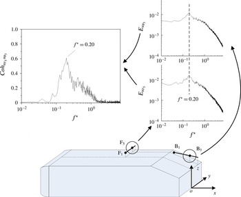
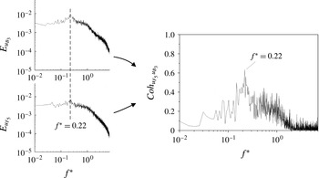
The fact that the unsteady structures detected over the rear window at $y^{\ast }=0{-}0.36$ (figures 3 and 5) occur at the same frequency ( $\mathit{St}_{r}=0.20$ ) as those above the roof (figure 17) suggests a connection between them. The spectral coherence $\mathit{Coh}_{u_{{\it\beta}}u_{{\it\gamma}}}~(\equiv (\mathit{Co}_{u_{{\it\beta}}u_{{\it\gamma}}}^{2}+Q_{u_{{\it\beta}}u_{{\it\gamma}}}^{2})/E_{u_{{\it\beta}}}E_{u_{{\it\gamma}}\!})$ is thus examined, where signals $u_{{\it\beta}}$ and $u_{{\it\gamma}}$ were simultaneously measured using two single hot wires, one placed above the roof and the other over the rear window, and $\mathit{Co}_{u_{{\it\beta}}u_{{\it\gamma}}}$ and $Q_{u_{{\it\beta}}u_{{\it\gamma}}}$ are the cospectrum and quadrature spectrum of $u_{{\it\beta}}$ and $u_{{\it\gamma}}$ , respectively. The coherence $\mathit{Coh}_{u_{{\it\beta}}u_{{\it\gamma}}}$ provides a measure for the quantitative correlation between the spectral components of $u_{{\it\beta}}$ and $u_{{\it\gamma}}$ (Antonia, Zhou & Matsumara Reference Antonia, Zhou and Matsumara1993). As illustrated in figure 18, both $E_{u_{{\it\beta}_{3}}}$ and $E_{u_{F_{5}}}$ of $u_{F_{5}}$ and $u_{B_{3}}$ , measured at $\text{F}_{5}$ and $\text{B}_{3}$ , respectively, display a predominant peak at the same frequency ( $\mathit{St}_{r}=0.20$ ). The $\mathit{Coh}_{u_{F_{5}}u_{B_{3}}}$ value shows a pronounced peak, reaching 0.63, at $f^{\ast }=\mathit{St}_{r}=0.20$ , indicating an excellent correlation between $u_{F_{5}}$ and $u_{B_{3}}$ at this frequency. The observation points to the fact that the shear layer development above the roof has a significant effect on flow separation and even vortex shedding from the slanted rear window. In fact, it may be concluded that the frequency of vortex shedding from the rear window is dictated by that of vortices generated behind the bubble near the leading edge of the roof.

Figure 18.

Spectral coherence between simultaneously measured hot-wire signals $u_{F_{5}}$ and  $u_{B_{3}}$ . Please refer to figures 3 and 17 for the locations of $\text{B}_{3}$ and $\text{F}_{5}$ .

The above finding prompts us to look at the shear layer developed over the side surface of the model. Figure 19 presents $E_{u}$ measured along $\text{E}_{1}{-}\text{E}_{5}~(x^{\ast }=-1.27,~y^{\ast }=0.63)$ near the side face. A pronounced peak occurs at $f^{\ast }=\mathit{St}_{l}=2.11$ at $\text{E}_{1}$ near the ground ( $z^{\ast }=0.14$ ). This predominant frequency is the same as that ( $\mathit{St}_{l}=2.11$ ) identified in $E_{u}$ measured at $\text{T}_{5}$ and $\text{T}_{6}$ (figure 15). Note that this $\mathit{St}_{l}$ corresponds to a dimensionless frequency of $\mathit{St}_{D}\approx 0.19$ and is approximately equal to the Strouhal number ( ${\approx}0.20$ ) in the wake of a circular cylinder. It may be inferred that the $\mathit{St}_{l}$ is the frequency of vortices generated by the struts located at $x^{\ast }=-2.52$ and $y^{\ast }=\pm 0.49$ between the model underside and the floor.

Figure 19.

Power spectral density function $E_{u}$ of the hot-wire signal measured along $\text{E}_{1}{-}\text{E}_{5}~(x^{\ast }=-1.27,~y^{\ast }=0.63)$ near the side surface.

Another predominant peak occurs at $f^{\ast }=\mathit{St}_{s}=0.27$ over $z^{\ast }=0.14{-}0.79$ . Grandemange, Gohlke & Cadot (Reference Grandemange, Gohlke and Cadot2013) studied the flow around a square-back Ahmed body ( ${\it\varphi}=0^{\circ }$ ) at $\mathit{Re}=1.1\times 10^{5}$ based on the surface pressure measurements in the ( $x,y$ ) plane at $z^{\ast }=0.43$ . They observed that the flow separated and then reattached near the leading edge of the side face, forming a recirculation bubble located roughly at $-3.0<x^{\ast }<-2.6$ . 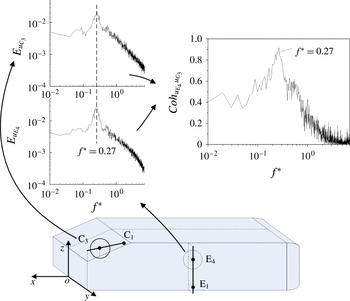Like the hairpin vortex observed above the roof, the side vortex is a structure emanated from the recirculation bubble that occurs near the leading edge of the side face. 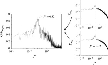Since the predominant unsteady structures at $\mathit{St}_{s}=0.27$ are detected along the side edge of the rear window and over the side surface, we used two hot wires to measure simultaneously the flow at $\text{E}_{4}$ and $\text{C}_{3}$ (figure 20). The spectral coherence $\mathit{Coh}_{u_{E_{4}}u_{C_{3}}}$ between $u_{E_{4}}$ and $u_{C_{3}}$ , obtained at $\text{E}_{4}$ and $\text{C}_{3}$ , respectively, shows a pronounced peak, with its magnitude reaching 0.92, at $f^{\ast }=\mathit{St}_{s}=0.27$ , indicating a near perfect correlation between $u_{E_{4}}$ and $u_{C_{3}}$ at this frequency. It is evident that the vortex frequency $\mathit{St}_{s}=0.27$ detected along the side edge of the slant surface is dictated by that of the side vortices formed over the side face of the Ahmed model.

Figure 20.

Spectral coherence between simultaneously measured hot-wire signals $u_{E_{4}}$ and $u_{C_{3}}$ . Please refer to figures 3 and 19 for the locations of $\text{C}_{3}$ and $\text{E}_{4}$ .

5. Reynolds number effect

The $\mathit{Re}$ effect on the flow has not been well addressed in the literature. The Ahmed model is designed to minimize flow separation from its fore-body and to have fixed flow separation from its after-body, which is characterized by clearly defined corners. Nevertheless, Minguez et al.’s (Reference Minguez, Pasquetti and Serre2008) LES at $\mathit{Re}=8.9\times 10^{5}$ showed that flow separated at the fore-body and then reattached on the roof and lateral sides, forming a bubble. The observation suggests a dependence of the flow structure on Re. Previously reported drag coefficient and Strouhal number data also display a variation with different Re (e.g. Vino et al. Reference Vino, Watkins, Mousley, Watmuff and Prasad2005; Thacker et al. Reference Thacker, Aubrun, Leroy and Devinant2010; Joseph et al. Reference Joseph, Amandolese and Aider2012). In this section, we will examine the possible dependence on Re of the Strouhal numbers based on hot-wire measurements conducted over a range of $U_{\infty }$ from 6 to $32~\text{m}~\text{s}^{-1}$ , with an increment of $2~\text{m}~\text{s}^{-1}$ in $U_{\infty }$ , corresponding to the Re range of $(0.45{-}2.4)\times 10^{5}$ .

Figure 21 presents the variation of the captured five Strouhal numbers, $\mathit{St}_{r}$ , $\mathit{St}_{s}$ , $\mathit{St}_{w}$ , $\mathit{St}_{g}$ and $\mathit{St}_{l}$ , with Re. The previously reported St for the Ahmed model of ${\it\varphi}=25^{\circ }$ is also included. Boucinha et al. (Reference Boucinha, Weber and Kourta2011) detected from hot-wire measurements $\mathit{St}=0.18$ above the rear window and $\mathit{St}=0.36$ behind the base at $\mathit{Re}=2.3\times 10^{5}$ . Minguez et al.’s (Reference Minguez, Pasquetti and Serre2008) data, i.e. $\mathit{St}=0.27$ above the rear window and $\mathit{St}=0.42$ behind the base, were obtained from numerical simulation at $\mathit{Re}=8.9\times 10^{5}$ . Joseph et al. (Reference Joseph, Amandolese and Aider2012) reported, based on hot-wire data, a significant rise in St from 0.33 to 0.50 over the rear window, but a slight increase from 0.51 to 0.53 behind the base, with Re increasing from $4.5\times 10^{5}$ to $6.8\times 10^{5}$ . If their St measured above the rear window and behind the base are interpreted as $\mathit{St}_{r}$ and $\mathit{St}_{w}$ , respectively, we see a qualitative agreement between the data. For example, $\mathit{St}_{r}$ rises with increasing Re. The deviation of these reports from each other and from ours is not unexpected in view of all the differences in techniques, experimental facilities, flow conditions, etc.

Figure 21.

Dependence on Re of the Strouhal numbers: $\mathit{St}_{r}$ (♢); $\mathit{St}_{s}$ (▫); $\mathit{St}_{w}$ (○); $\mathit{St}_{g}$ (▿); $\mathit{St}_{l}$ (▵). The three pairs of symbols ♦ and ●, and 

and 

, denote $\mathit{St}_{r}$ and $\mathit{St}_{w}$ , respectively, measured by Joseph et al. (Reference Joseph, Amandolese and Aider2012) and Boucinha et al. (Reference Boucinha, Weber and Kourta2011), respectively.

Both $\mathit{St}_{r}$ and $\mathit{St}_{s}$ display approximately linear rise with increasing Re. The data fit reasonably well to the equation $\mathit{St}=\mathit{St}^{\prime }+m\mathit{Re}$ , where constants $\mathit{St}^{\prime }$ and $m$ , given in figure 21, are determined from the least-squares fitting to experimental data. The similar behaviour between $\mathit{St}_{r}$ and $\mathit{St}_{s}$ is internally consistent with the fact that their physical origins are the same, as found in § 4, both connected to vortices emanated from the recirculation bubble formed near the leading edge of the roof or side surface. In flow around a rectangular flat plate, the frequency $f$ of vortices emanated from the recirculation bubble was found to scale with $U_{\infty }/x_{R}$ (Kiya & Sasaki Reference Kiya and Sasaki1985; Tafti & Vanka Reference Tafti and Vanka1991). It may be inferred that the frequency $f_{j}~(\,j\in \{r~\mathit{or}~s\})$ of vortices emanated from the recirculation bubble near the leading edge of the roof or the side surface of the model is dictated by

(5.1) $$\begin{eqnarray}f_{j}\sim U_{\infty }/x_{Rj},\end{eqnarray}$$

where $x_{Rj}$ is the length of the bubble. Then, $\mathit{St}_{j}$ may be rewritten as

(5.2) $$\begin{eqnarray}\mathit{St}_{j}\sim (U_{\infty }/x_{Rj})\sqrt{A}/U_{\infty }=\sqrt{A}/x_{Rj}=1/x_{Rj}^{\ast },\quad j\in \{r~\mathit{or}~s\}.\end{eqnarray}$$

Grandemange et al. (Reference Grandemange, Gohlke and Cadot2013) studied the flow around an Ahmed body ( ${\it\varphi}=0^{\circ }$ ) based on surface pressure measurements, and found that the recirculation bubbles ( $x_{R}^{\ast }$ ) near the leading edge of the roof and side surface contracted in length from 0.4 to 0.04, with Re increasing from $1.1\times 10^{5}$ to $2.9\times 10^{6}$ . Evidently, the rise in $\mathit{St}_{r}$ and $\mathit{St}_{s}$ for higher Re (figure 21) is attributed to a contraction in $x_{R}^{\ast }$ . Based on flow visualization in a water tunnel, Spohn & Gillieron (Reference Spohn and Gillieron2002) observed that the recirculation bubble formed near the leading edge of the roof was three-dimensional. The $x_{R}$ value was largest in the symmetry plane ( $y^{\ast }=0$ ) and retreated towards the side surface, down to $x_{R}=0$ at each end of the separation line. Note that the width of the roof ( $W^{\ast }=1.16$ ) is different from the height of the side surface ( $H^{\ast }=0.86$ ), which may cause a difference in size between the bubbles above the roof and on the lateral side and hence may be responsible for the different slopes in $\mathit{St}_{r}$ and $\mathit{St}_{s}$ versus Re.

The unsteady structures responsible for $\mathit{St}_{w}$ arise from a mechanism very different from that for $\mathit{St}_{r}$ and $\mathit{St}_{s}$ , their generation being connected to the recirculation bubbles behind the vertical base (§ 3.3). As such, the dependence on Re of $\mathit{St}_{w}$ is rather distinct from those of $\mathit{St}_{r}$ and $\mathit{St}_{s}$ and the nonlinearity is quite appreciable.

Figure 22.

Spectral coherence between simultaneously measured hot-wire signals $u_{F_{5}}$ and $u_{B_{3}}$ at $\mathit{Re}=1.2\times 10^{5}$ . Please refer to figures 3 and 17 for the locations of $\text{B}_{3}$ and $\text{F}_{5}$ .

The values of $\mathit{St}_{l}$ and $\mathit{St}_{g}$ are 2.12 and 1.77, respectively, and vary little for the Re range examined (figure 21). As discussed earlier, the two frequencies are ascribed to vortices generated by the cylindrical struts located at $x^{\ast }=-2.52$ and $y^{\ast }=\pm 0.49$ and $x^{\ast }=-1.11$ and $y^{\ast }=\pm 0.49$ , respectively. The results are internally consistent with the fact that the Strouhal number in the wake of a circular cylinder remains nearly constant, i.e. $\mathit{St}_{D}\approx 0.2$ , for $\mathit{Re}_{D}=3.0\times 10^{2}$ to $1.0\times 10^{5}$ (e.g. Schlichting & Gersten Reference Schlichting and Gersten2000). The value of $\mathit{St}_{g}$ is lower than that of $\mathit{St}_{l}$ by approximately 16 % since the fluid between the floor and the model underside is decelerated on moving downstream due to the boundary layers formed over both the floor and the model underside.

The predominant peak at $\mathit{St}_{a}$ in $\mathit{E}_{u}$ , such as the peak at $f^{\ast }=0.14$ in figure 17, is not evident any more as Re exceeds $1.0\times 10^{5}$ (not shown). At higher Re, the separation bubble near the leading edge of the roof (§ 4) is reduced in length (Grandemange et al. Reference Grandemange, Gohlke and Cadot2013), and its pulsation is thus attenuated. Naturally, the oscillation of the longitudinal vortex core may be impaired and may even vanish, accounting for the disappearance of $\mathit{St}_{a}$ .

As illustrated in figure 22, at $\mathit{Re}=1.2\times 10^{5}$ , both $E_{u_{B_{3}}}$ and $E_{u_{F_{5}}}$ display a predominant peak at the same frequency ( $\mathit{St}_{r}=0.22$ ), where hot-wire signals $u_{F_{5}}$ and $u_{B_{3}}$ are simultaneously measured at $\text{F}_{5}$ above the roof (figure 17) and $\text{B}_{3}$ (figure 3 b) over the rear window. The $\mathit{Coh}_{u_{F_{5}}u_{B_{3}}}$ value shows a pronounced peak, reaching 0.62 at this frequency. The $\mathit{Coh}_{u_{E_{4}}u_{C_{3}}}$ between $u_{E_{4}}$ and $u_{C_{3}}$ (figure 23) simultaneously obtained at $\text{E}_{4}$ over the side surface (figure 19) and $\text{C}_{3}$ near the side edge of the rear window (figure 3 c) at $\mathit{Re}=1.2\times 10^{5}$ , respectively, displays a pronounced peak, with its magnitude reaching 0.92, at $\mathit{St}_{s}=0.32$ . Both $E_{u_{L_{1}}}$ and $E_{u_{L_{4}}}$ (figure 24) of $u_{L_{1}}$ and $u_{L_{4}}$ simultaneously measured at $\text{L}_{1}$ and $\text{L}_{4}$ in the symmetry plane behind the base (figure 7) exhibit a predominant peak at $\mathit{St}_{w}=0.50$ , which is ascribed to the organized structures emanated from the upper and lower recirculation bubbles behind the base. Similarly to the observation made at $\mathit{Re}=0.62\times 10^{5}$ (figure 9 a), the spectral phase shift ${\it\Phi}_{u_{L_{1}}u_{L_{4}}}$ between $u_{L_{1}}$ and $u_{L_{4}}$ is near ${\rm\pi}$ at $\mathit{St}_{w}=0.50$ , indicating an antiphase relationship. By comparing the results at $\mathit{Re}=1.2\times 10^{5}$ with those at $\mathit{Re}=0.62\times 10^{5}$ , it may be concluded that the Re effect on the connections between structures at different locations is insignificant.

Figure 23.

Spectral coherence between simultaneously measured hot-wire signals $u_{E_{4}}$ and $u_{C_{3}}$ at $\mathit{Re}=1.2\times 10^{5}$ . Please refer to figures 3 and 19 for the locations of $\text{C}_{3}$ and $\text{E}_{4}$ .

Figure 24.

Spectral phase between hot-wire signals simultaneously measured at $\text{L}_{1}$ and $\text{L}_{4}$ at $\mathit{Re}=1.2\times 10^{5}$ . Please refer to figure 7 for the locations of $\text{L}_{1}$ and $\text{L}_{4}$ .

6. Turbulent intensity effect

The values of $E_{u}$ (figure 25) measured at $T_{u}=7.8\,\%$ for $\mathit{Re}=0.62\times 10^{5}$ exhibit a number of changes from their counterparts measured at $T_{u}=0.3\,\%$ (figures 5 b, 7, 15, 17 a and 19). Firstly, there is no pronounced spectral peak in $E_{u}$ measured at $\text{D}_{1}{-}\text{D}_{5}~(x^{\ast }=-2.33,~z^{\ast }=0.95)$ near the leading edge of the roof (figure 25). In comparison, $E_{u}$ measured at the same locations at $T_{u}=0.3\,\%$ (figure 17 a) displays two predominant frequencies, i.e. $\mathit{St}_{r}=0.20$ at $y^{\ast }=0$ and over $y^{\ast }=0.29{-}0.36$ , and $\mathit{St}_{a}=0.14$ over $y^{\ast }=0.14{-}0.22$ , respectively. The former is attributed to the vortices emanated from the recirculation bubble near the leading edge of the roof, and the latter to the oscillation of the core of longitudinal vortices originated from bubble pulsation. The observation is fully consistent with previous reports in the literature. Conan, Anthoine & Planquart (Reference Conan, Anthoine and Planquart2011) performed oil visualization measurements on the front of an Ahmed body at $\mathit{Re}=8.9\times 10^{5}$ , and observed a flow separation region near the leading edge of the roof. They then deployed a strip of sandpaper before the separation line to force the transition to turbulence. As a result, flow separation was suppressed. Wang et al. (Reference Wang, Zhou, Alam and Yang2014) studied the effect of $T_{u}$ on the flow structures around an aerofoil at different angles ( ${\it\alpha}$ ) of attack. At ${\it\alpha}=5^{\circ }{-}12^{\circ }$ , they found that the increased $T_{u}$ acted to promote the shear layer transition after flow separation near the leading edge, and the separation bubble was significantly suppressed. It may be concluded that the recirculation bubble near the leading edge of the roof must have been suppressed at $T_{u}=7.8\,\%$ . Consequently, $E_{u}$ measured at $\text{D}_{1}{-}\text{D}_{5}$ exhibits no pronounced peaks. By the same token, the spectral peak at $\mathit{St}_{s}=0.27$ observed for $T_{u}=0.3\,\%$ in $E_{u}$ (figure 19) vanishes at $T_{u}=7.8\,\%$ (figure 25) since the recirculation bubble near the leading edge of the side face is also suppressed at the higher $T_{u}$ .

Figure 25.

Power spectral density function $E_{u}$ of the hot-wire signal measured around the model at $T_{u}=7.8\,\%$ . Please refer to figures 5, 7, 15, 17 and 19 for the locations of $\text{H}_{1}{-}\text{H}_{5}$ , $\text{L}_{1}{-}\text{L}_{5}$ , $\text{T}_{1}{-}\text{T}_{5}$ , $\text{D}_{1}{-}\text{D}_{5}$ and $\text{E}_{1}{-}\text{E}_{5}$ , respectively.

Secondly, a rather broad hump occurs over $f^{\ast }=0.1{-}0.3$ in $E_{u}$ measured at $\text{H}_{1}{-}\text{H}_{5}~(x^{\ast }=-0.17,~z^{\ast }=0.79)$ and $y^{\ast }=0{-}0.29$ over the rear window at $T_{u}=7.8\,\%$ , in contrast to the less broad peak at $\mathit{St}_{r}=0.20$ in $E_{u}$ measured over $y^{\ast }=0{-}0.36$ at $T_{u}=0.3\,\%$ (figure 5), which is attributed to the spanwise vortices emanated from the separation bubble at the upper edge of the rear window. It was earlier found that this frequency is dictated by that of the vortices emanated from the separation bubble near the leading edge of the roof. It may be inferred that the spanwise vortices may form less periodically without the upstream vortex excitation at $T_{u}=7.8\,\%$ .

Thirdly, the quasi-periodic structures at $\mathit{St}_{w}=0.44$ alternately emanated from the upper and lower recirculation bubbles behind the base at $T_{u}=0.3\,\%$ (figure 7) remain at $T_{u}=7.8\,\%$ ; a pronounced peak is evident at $f^{\ast }=\mathit{St}_{w}=0.44$ in $E_{u}$ (figure 25) measured along $\text{L}_{1}{-}\text{L}_{5}~(x^{\ast }=0.4,~y^{\ast }=0)$ behind the base.

Finally, the flow structures associated with $\mathit{St}_{l}=2.12$ and $\mathit{St}_{g}=1.77$ , detected at $T_{u}=0.3\,\%$ near the lower edge of the side surface and behind the lower edge of the base, respectively (figures 15 and 19), are also identifiable at $T_{u}=7.8\,\%$ . As shown in figure 25, $E_{u}$ measured along $\text{E}_{1}{-}\text{E}_{5}~(x^{\ast }=-1.27,~y^{\ast }=0.63)$ near the side surface displays a predominant peak at $f^{\ast }=\mathit{St}_{l}=2.11$ at $z^{\ast }=0.14$ near the floor, and that along $\text{T}_{1}{-}\text{T}_{5}~(x^{\ast }=0.09,~z^{\ast }=0)$ behind the lower edge of the base shows a peak at $f^{\ast }=\mathit{St}_{l}=1.76$ over $y^{\ast }=0.5{-}0.65$ . The slight deviation in $\mathit{St}_{l}$ and $\mathit{St}_{g}$ between the two cases is well within experimental uncertainties.

7. A conceptual model of the flow structure

A conceptual model is proposed for the flow structure of the high-drag regime around the Ahmed model ( ${\it\varphi}=25^{\circ }$ ), as sketched in figure 26, based on the present data and those in the literature. This model covers the flow structure above the roof, over the side surface and the rear window, and behind the base, including all the indicative predominant frequencies of the unsteady structures.

Figure 26.

A conceptual model of the flow structure around the Ahmed model.

The flow separates and then reattaches near the leading edge of the roof, producing a periodically pulsating recirculation bubble (Minguez et al. Reference Minguez, Pasquetti and Serre2008). Two predominantly longitudinal counter-rotating vortices occur behind the bubble, whose origin is two foci at the ends of the flow separation line (Spohn & Gillieron Reference Spohn and Gillieron2002). The longitudinal vortex core oscillates at a frequency of $\mathit{St}_{a}=0.14$ at $\mathit{Re}=0.62\times 10^{5}$ (figure 17 a), resulting from the bubble pulsation. The frequency $\mathit{St}_{r}=0.18{-}0.28$ in the Re range of $(0.45{-}2.4)\times 10^{5}$ (figures 17 a,b and 21) is linked to three-dimensional hairpin vortices (Krajnović & Davidson Reference Krajnović and Davidson2005a ; Franck et al. Reference Franck, Nigro, Storti and D’elia2009), which emanate from the recirculation bubble and advect downstream along the roof. Behind the recirculation bubble formed near the leading edge of the side surface, side vortices occur at a frequency $\mathit{St}_{s}=0.25{-}0.45$ given $\mathit{Re}=(0.45{-}2.4)\times 10^{5}$ (figures 19 and 21).

The bubble pulsation and hairpin vortex emanation bear similarity to observations in flow around a blunt flat plate. The bubble in flow around a blunt flat plate is characterized by periodic enlargement and shrinkage, i.e. bubble pulsation, and the shear layer rolls up behind the bubble, forming vortices. Kiya & Sasaki (Reference Kiya and Sasaki1985) captured experimentally two distinct frequencies, i.e. $0.12U_{\infty }/x_{R}$ and $0.65U_{\infty }/x_{R}$ , which were ascribed to the recirculation bubble pulsation and vortex emanation from the bubble, respectively. Tafti & Vanka (Reference Tafti and Vanka1991) extracted numerically the recirculation bubble pulsation frequency at $0.15U_{\infty }/x_{R}$ and the vortex emanation frequency at $0.6U_{\infty }/x_{R}$ . Spohn & Gillieron (Reference Spohn and Gillieron2002) also reported experimentally the frequency of vortex emanation from the bubble, which exceeded 10 times the pulsation frequency of the recirculation bubble. Note that the bubble pulsation frequency reported by Kiya & Sasaki (Reference Kiya and Sasaki1985) and Tafti & Vanka (Reference Tafti and Vanka1991) is of the order of one-quarter of the vortex emanation frequency, smaller than ours, which is approximately three-quarters. Such a discrepancy may be linked to a difference in the geometry of the leading edge of the model and the three-dimensionality, as discussed earlier, of the recirculation bubble between theirs and ours.

Photographs from flow visualization (figure 4) indicate that flow separates from the upper sharp edge of the rear window and then reattaches on the slant surface, forming a very small recirculation bubble. This bubble grows with increasing ${\it\varphi}$ (Conan et al. Reference Conan, Anthoine and Planquart2011) and bursts when ${\it\varphi}$ reaches $30^{\circ }$ (Ahmed et al. Reference Ahmed, Ramm and Faltin1984). The previously observed quasi-periodic spanwise vortices over the rear window (Wang et al. Reference Wang, Zhou, Pin and Chan2013) are found with a predominant frequency of $\mathit{St}_{r}=0.18{-}0.28$ for the Re range of $(0.45{-}2.4)\times 10^{5}$ , as determined from the hot-wire signal spectrum measured over $y^{\ast }=0{-}0.36$ (figure 5). It is further found that the spanwise vortices are connected to the hairpin vortices formed behind the separation bubble near the leading edge of the roof. In fact, the two unsteady structures are highly correlated, with the predominant frequency of the former dictated by that of the latter (figure 18). This connection suggests that the shear layer formed above the roof has a significant impact on flow separation and vortex shedding from the slanted rear window. The shear layer rolls up about the side edge of the slant surface due to the pressure difference between the flow coming off the side surface and that over the rear window, thus forming the C-pillar vortices (Ahmed et al. Reference Ahmed, Ramm and Faltin1984). On the other hand, the side vortices are formed at $\mathit{St}_{s}=0.25{-}0.45$ , for $\mathit{Re}=(0.45{-}2.4)\times 10^{5}$ , over the side surface of the model. Under the rollup effect of the shear layer coming off the side surface along the side edge of the rear window, the side vortices are probably wrapped up around the slanted side edge. This may explain why $\mathit{St}_{s}$ is detected where the C-pillar vortex occurs (figures 3 c, 5 and 21).

One row of alternately signed streamwise structures occurs at the same level of the upper edge of the base. The C-pillar vortex induces the adjacent longitudinal vorticity concentration of opposite sign, which is considerably weaker. For the same reason, another vorticity concentration of even weaker strength can be induced next to this secondary vortex.

The shear layers roll up at the upper and lower edges of the vertical base, forming the upper and lower recirculation bubbles. The coherent structures are alternately emanated at $\mathit{St}_{w}=0.44{-}0.54$ for $\mathit{Re}=(0.45{-}2.4)\times 10^{5}$ from the two bubbles in the central region of the wake (figures 8 and 21). The structure from the upper bubble appears sweeping towards the ground and then breaking up, whilst that from the lower bubble is emanated upwards. The latter is found to persist significantly longer than the former and grows downstream with spanwise extent increasing, as inferred from the power spectral density function of the hot-wire signals (figure 7) and the spectral phase shift between the signals (figure 9). The C-pillar vortex and the upper recirculation bubble interact with each other and merge downstream, forming one pair of counter-rotating trailing vortices in the wake (figure 14). The previously observed lower vortex (Krajnović & Davidson Reference Krajnović and Davidson2005a ), gap vortex and side vortex (Wang et al. Reference Wang, Zhou, Pin and Chan2013) are all incorporated in this model. The lower vortex is formed near the lower edge of the side surface due to the pressure difference between the flow inside and outside the gap between the model underside and the floor (e.g. Wang et al. Reference Wang, Zhou, Pin and Chan2013). The unsteady structures at $\mathit{St}_{l}\approx 2.12$ are detected near the lower edge of the side surface (figures 19 and 21), which are generated by the upstream struts located at $x^{\ast }=-2.52$ and $y^{\ast }=\pm 0.49$ . On the other hand, the gap vortex is generated by the downstream struts located at $x^{\ast }=-1.11$ and $y^{\ast }=\pm 0.49$ , and its predominant frequency is $\mathit{St}_{g}\approx 1.77$ (figures 15 and 21).

The flow structures shown in figure 26 are all obtained based on instantaneous data. It should be noted that some instantaneous flow structures, e.g. the pair of C-pillar vortices, and the upper and lower recirculation bubbles behind the base, remain after the time-averaging process, as is evident in the classical Ahmed time-averaged flow structure model (Ahmed et al. Reference Ahmed, Ramm and Faltin1984), while others, e.g. the alternately emanated organized structures from the upper and lower recirculation bubbles behind the base and the spanwise vortex rolls over the slanted surface, may disappear due to a jitter or change in their spatial locations during the time-averaging process.

Instantaneous flow structures, including the vortices emanated from the recirculation bubbles formed near the leading edge of the roof and side surface, and the pair of longitudinal vortices originating from two foci at each end of the separation line near the leading edge of the roof, fail to be detected at $\mathit{Re}>2.4\times 10^{5}$ . Based on the surface pressure measurements, Grandemange et al. (Reference Grandemange, Gohlke and Cadot2013) found that the recirculation bubbles near the leading edge of the roof and side surface shrunk significantly in length with increasing Re. Apparently, the vanishing of these vortices is connected to the suppressed recirculation bubbles with increasing Re. This observation bears similarity to that made as $T_{u}$ is increased at $\mathit{Re}=0.62\times 10^{5}$ , where the two vortex frequencies, i.e. $\mathit{St}_{r}=0.20$ and $\mathit{St}_{s}=0.27$ , captured at $T_{u}=0.3\,\%$ over the roof and the side face, respectively, cannot be detected at $T_{u}=7.8\,\%$ (figure 25). Wang et al. (Reference Wang, Zhou, Alam and Yang2014) found that, at a low Reynolds number $\mathit{Re}_{c}$ , based on the chord length of the aerofoil, the influence of $T_{u}$ on the aerofoil wake exhibited similarity to that of $\mathit{Re}_{c}$ . For example, both $T_{u}$ and $\mathit{Re}_{c}$ , if increased, could cause early transition in the shear layer and hence reattachment, forming a separation bubble. The concept of the effective Reynolds number was proposed, which treated $T_{u}$ as an additional $\mathit{Re}_{c}$ , with a caveat that the two effects are not identical in every aspect. It seems plausible based on the present observations that $T_{u}$ may be treated as an additional Re in the Ahmed model wake, though more experimental data are required to document the similarity and differentiation between the two effects.