1 Introduction
A small particle moving in a shear flow experiences a lift force due to the shear effect. The lift force is of great importance in a wide range of areas, such as aerosol technology (McLaughlin Reference McLaughlin1989; Zhao et al.
Reference Zhao, Zhang, Li, Yang and Huang2004), inhalation toxicology (Kleinstreuer, Zhang & Donohue Reference Kleinstreuer, Zhang and Donohue2008a
), chemical engineering (Massoudi Reference Massoudi2002) and environmental science (Zou et al.
Reference Zou, Cheng, Zhang and Zhao2007). Over the past decades, extensive studies have been carried out on the lift forces for small particles in gaseous media. The particles of practical interest are usually non-spherical. The general simplified way to study the transport properties of non-spherical particles is to introduce its spherical equivalent or a shape factor parameter (Saffman Reference Saffman1965; Cherukat & McLaughlin Reference Cherukat and McLaughlin1994; Asmolov Reference Asmolov1999; Kröger & Hütter Reference Kröger and Hütter2006a
; Liu & Bogy Reference Liu and Bogy2008, Reference Liu and Bogy2009; Loth Reference Loth2008; Zheng & Silber-Li Reference Zheng and Silber-Li2009; Kleinstreuer & Feng Reference Kleinstreuer and Feng2013; Luo et al.
Reference Luo, Wang, Xia and Li2016a
,Reference Luo, Wang, Xia and Li
b
; Yang, Bian & Wang Reference Yang, Bian and Wang2017). However, this method lacks rigour and may give misleading predictions. The influence of the geometric shape and orientation on the lift cannot be neglected. A slender particle is one of the most common non-spherical particles. The lift on a slender particle is very different from that on an equivalent sphere because of both the non-spherical shape and the orientation effect of the slender particle. So far, available works on lift force for slender particles are limited to microsized particles (Kröger & Hütter Reference Kröger and Hütter2006a
,Reference Kröger and Hütter
b
; Wang et al.
Reference Wang, Yu, Luo, Xia and Zong2018). Nanosized slender particles (NSPs), including nanotubes, nanorods and fibrous aerosols, are considered as nanocylinders in the present paper. Some large molecules (for example, long-chain
 $n$
-alkane) can also be roughly approximated as small cylinders (Garcia-Ybarra & Rosner Reference Garcia-Ybarra and Rosner1989; Liu, Li & Wang Reference Liu, Li and Wang2016a
; Liu et al.
Reference Liu, McGivern, Manion and Wang2016b
, Reference Liu, Zhao, Xu, Egolfopoulos and Wang2017). The lift of these nanocylinders in shear flows can find applications in many industrial, physiological and technological processes, including materials synthesis, combustion of
 $n$
-alkane flames, drug delivery, and the characterization of nanotubes (Gavze & Shapiro Reference Gavze and Shapiro1998; Yin et al.
Reference Yin, Rosendahl, Kær and Sørensen2003; Kleinstreuer, Zhang & Li Reference Kleinstreuer, Zhang and Li2008b
; Högberg et al.
Reference Högberg, Åkerstedt, Lundström and Freund2010; Ji et al.
Reference Ji, Dames, Wang, Wang and Egolfopoulos2010; Feng & Kleinstreuer Reference Feng and Kleinstreuer2013; Kleinstreuer & Feng Reference Kleinstreuer and Feng2013; Dong & Cao Reference Dong and Cao2014, Reference Dong and Cao2015). One such case is the motion of carbon nanotubes (CNTs) in small channels (for example, in the human respiratory tract), where the lift force may significantly affect the deposition and rotation of the CNTs (Kleinstreuer et al.
Reference Kleinstreuer, Zhang and Li2008b
; Högberg et al.
Reference Högberg, Åkerstedt, Lundström and Freund2010; Feng & Kleinstreuer Reference Feng and Kleinstreuer2013; Kleinstreuer & Feng Reference Kleinstreuer and Feng2013). Therefore, it is of considerable interest to investigate the lift force on nanocylinders in shear flows.
In gaseous media, the lift force on the cylinder strongly depends on the Knudsen number,
 $Kn=\unicode[STIX]{x1D706}/R$
, where
 $\unicode[STIX]{x1D706}$
is the mean free path of the gas and
 $R$
is the cylinder radius. In the continuum regime (
 $Kn\ll 1$
), classical fluid mechanics theory can be employed to study the lift force. The lift force in this regime arises from the small inertia effects (Cherukat & McLaughlin Reference Cherukat and McLaughlin1994; Asmolov Reference Asmolov1999). Theoretical solutions of the lift force can be obtained by analysing the inertial terms in the Navier–Stokes equation by using perturbation methods. Jeffery (Reference Jeffery1922) pioneered work on the motion of cylindrical particles in shear flows in the continuum limit. Later, Jeffery’s work was extended to a more general class of particle shapes (Bretherton Reference Bretherton1962; Cox Reference Cox1971; Leal Reference Leal1980). Harper & Chang (Reference Harper and Chang1968) obtained the lift force acting on an arbitrarily shaped particle by generalizing Saffman’s results for the lift force on a sphere moving in a linear shear flow (Saffman Reference Saffman1965). The expressions for lift forces given by Harper and Chang have been widely used in numerical simulations of the transport of cylindrical particles in shear flows (Fan et al.
Reference Fan, Soltani, Ahmadi and Hart1997; Fan & Ahmadi Reference Fan and Ahmadi2000; Tian et al.
Reference Tian, Ahmadi, Wang and Hopke2012).
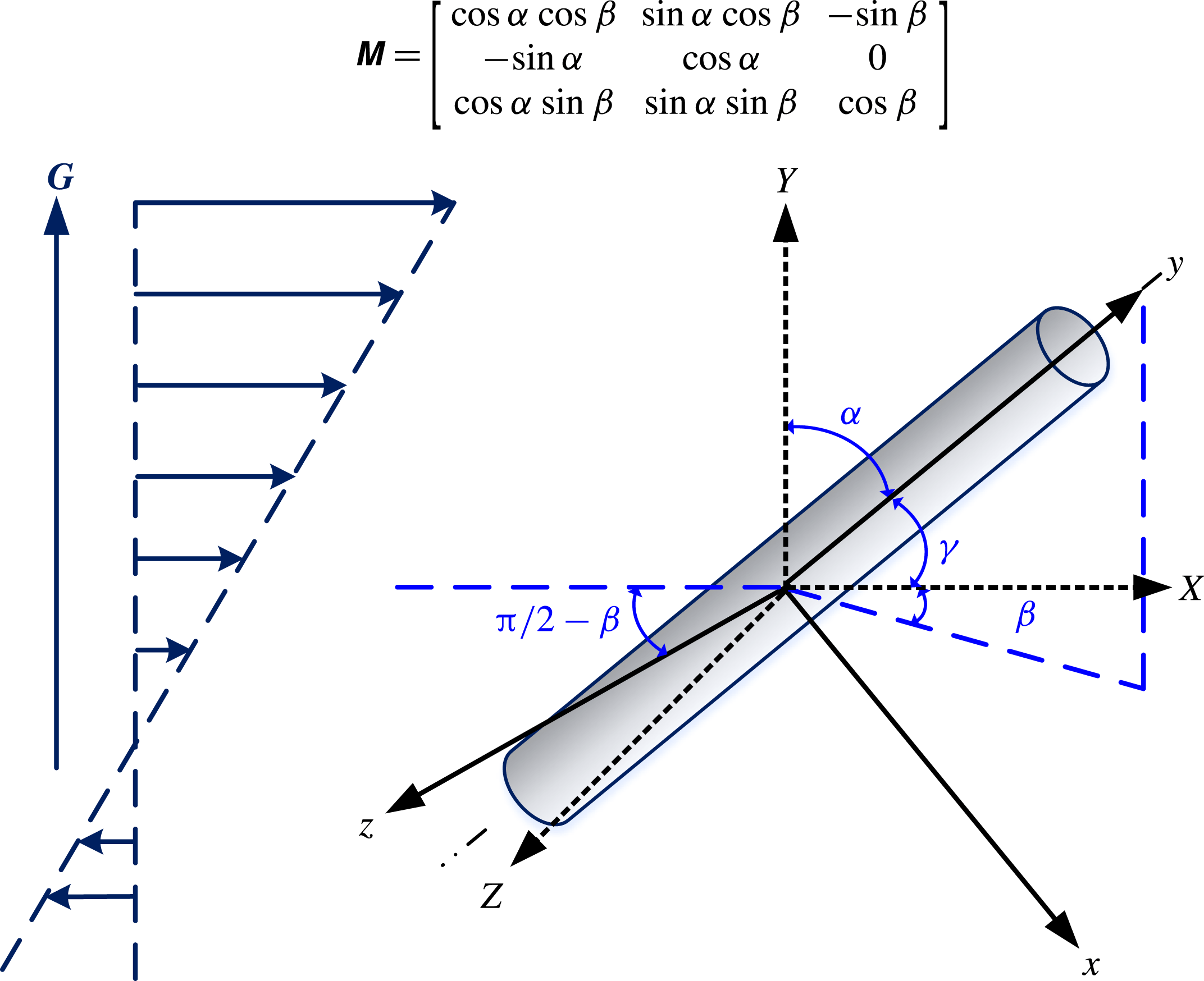
Schematic of a cylinder in a linear shear flow and the coordinate systems.

In the free molecule regime, the mean free path of the surrounding gas is much larger than the characteristic length of the particle. The continuum hypothesis is invalid in this regime and the gas kinetic theory should be employed to analyse the lift forces. At standard conditions, the mean free path of a gas is approximately 100 nm. Thus, for cylinders with a radius of 10 nm or below, the flow regime is definitely in the free molecule regime. The theoretical analysis can be greatly simplified by recognizing that the influence of the presence of the cylinder on the velocity distribution of the gas molecules can be neglected. In the free molecule regime, studies on the lift force in the literature are limited primarily due to the complicated dependence of the lift force on the cylinder shape and orientation. Kröger & Hütter (Reference Kröger and Hütter2006a ,Reference Kröger and Hütter b ) investigated the lift force on a cylinder in a shear flow of a rarefied gas via algebraic manipulations. Recently, we performed a gas kinetic theory analysis and derived the lift force on a non-spherical particle moving in a linear shear flow for rigid-body collisions (Wang et al. Reference Wang, Yu, Luo, Xia and Zong2018). For a cylinder, the lift force is given by
 $$\begin{eqnarray}\boldsymbol{F}_{L}=-{\displaystyle \frac{5\unicode[STIX]{x03C0}}{32}}\unicode[STIX]{x1D70C}\unicode[STIX]{x1D706}RLU_{0}\boldsymbol{G}\left[2\unicode[STIX]{x1D70E}_{\unicode[STIX]{x1D70F}}\sin ^{2}\unicode[STIX]{x1D6FE}+\left(2-\unicode[STIX]{x1D70E}_{p}-{\displaystyle \frac{3\unicode[STIX]{x1D70E}_{\unicode[STIX]{x1D70F}}}{2}}\!\right)\!(3\cos ^{2}\unicode[STIX]{x1D6FE}\cos ^{2}\unicode[STIX]{x1D6FC}+\sin ^{2}\unicode[STIX]{x1D6FC}-\cos ^{2}\unicode[STIX]{x1D6FE})\right]\!,\end{eqnarray}$$
where
 $\unicode[STIX]{x1D70C}$
is the gas density,
 $\boldsymbol{G}$
is the velocity gradient,
 $U_{\text{0}}$
is the velocity of the flow relative to the cylinder,
 $L$
is the length of the cylinder,
 $\unicode[STIX]{x1D6FC}$
denotes the angle between the flow gradient and the axis of the cylinder,
 $\unicode[STIX]{x1D6FE}$
denotes the angle between the flow direction and the axis of the cylinder (see figure 1), and
 $\unicode[STIX]{x1D70E}_{\unicode[STIX]{x1D70F}}$
and
 $\unicode[STIX]{x1D70E}_{p}$
are the tangential and normal accommodation coefficients, which represent the fraction of gas molecules that are diffusely scattered. In general, accommodation coefficients are dependent on the gas–particle intermolecular interactions, the particle size and the temperature. There have been a number of studies on the accommodation coefficients (Millikan Reference Millikan1923; Allen & Raabe Reference Allen and Raabe1982; Li & Wang Reference Li and Wang2005, Reference Li and Wang2003b
; Prabha & Sathian Reference Prabha and Sathian2012; Jung et al.
Reference Jung, Han, Mulholland, Pui and Kim2013; Yamaguchi, Matsuda & Niimi Reference Yamaguchi, Matsuda and Niimi2017). These results show that the accommodation coefficients increase with increasing interaction strength of the gas–particle potential or decreasing temperature;
 $\unicode[STIX]{x1D70E}_{\unicode[STIX]{x1D70F}}=\unicode[STIX]{x1D70E}_{p}=0$
for specular scattering and
 $\unicode[STIX]{x1D70E}_{\unicode[STIX]{x1D70F}}=\unicode[STIX]{x1D70E}_{p}=1$
for diffuse scattering are two limiting cases. For large particles, 0.9 is traditionally used for the accommodation coefficients (Millikan Reference Millikan1923; Allen & Raabe Reference Allen and Raabe1982). Note that the lift force in (1.1) is proportional to gas density. Thus the lift force may not be very large when the gas is highly rarefied. However, the lift force becomes important if the shear rate is high. Several studies have demonstrated that the lift force is important for the migration and deposition of particles, especially in boundary layers or Couette flows (Liu & Bogy Reference Liu and Bogy2008, Reference Liu and Bogy2009; Loth Reference Loth2008; Zheng & Silber-Li Reference Zheng and Silber-Li2009). Equation (1.1) is different from the lift force formula derived by Harper & Chang (Reference Harper and Chang1968) in the continuum regime. This is due to the discrepancy in the mechanisms governing the lift force. In the continuum regime, the surrounding gas can be considered as a continuum medium, and the weak nonlinear convective interaction governs the lift force, whereas in the free molecule regime, the continuum assumption is invalid and the lift force results from momentum transfer upon collisions between the gas molecules and the cylinder.
The rigid-body collision assumption employed in the model of (1.1) neglects the intermolecular interactions (for example, van der Waals interactions) between the gas molecules and the suspended particle, which are important for nanoscale objects, as evidenced by recent theoretical (Li & Wang Reference Li and Wang2003a , Reference Li and Wang2004; Wang & Li Reference Wang and Li2011, Reference Wang and Li2012; Liu et al. Reference Liu, Li and Wang2016a ,Reference Liu, McGivern, Manion and Wang b ; Wang, Luo & Xia Reference Wang, Luo and Xia2017), experimental (Okada et al. Reference Okada, Nishiumi, Ueno, Kawabata and Kudoh2011; Zhang et al. Reference Zhang, Li, Yan and Yao2012; Laiho & Mustonen Reference Laiho, Mustonen, Ohno, Maruyama and Kauppinen2017) and numerical investigations (Li & Wang Reference Li and Wang2005). The transport of gas molecules and the resulting momentum transfer upon collisions with the nanocylinder can be substantially affected by non-rigid-body collisions. Our recent studies on the lift force acting on spherical nanoparticles have also shown that gas–particle interactions play an important role (Luo et al. Reference Luo, Wang, Xia and Li2016a ,Reference Luo, Wang, Xia and Li b ). Therefore, the rigid-body collision assumption used in (1.1) cannot be applied to nanocylinders. To accurately predict the lift forces on nanosized cylinders in shear flows of rarefied gases, it is necessary to develop a generalized lift force formula by taking into account the non-rigid-body effect.
In this paper, we investigate the effect of intermolecular interactions on the shear lift forces on nanocylinders in the free molecule regime. Based on the gas kinetic theory, the formulae for the lift forces are derived for both specular and diffuse scattering. The orientation effect of the cylinder is also taken into account. The current theoretical formulae can be reduced to those in the limit of rigid-body collisions. Theoretical analysis of the lift contributes to a more in-depth understanding of the transport behaviours of nanocylinders in shear flows.
The rest of the paper is organized as follows. The gas kinetic theory analysis of the lift force is conducted in § 2, wherein the velocity distribution function is presented. In § 3, we derive the formulae for the lift forces on nanocylinders in linear shear flows. The gas–cylinder intermolecular interactions are taken into account in the derivation. As examples, the lift forces on carbon nanotubes and long-chain
 $n$
-alkanes are evaluated in § 4. Finally, the paper is concluded in § 5.
2 Kinetic analysis and the velocity distribution
Figure 1 shows the schematic of a cylinder of radius
 $R$
and length
 $L$
moving in a linear shear flow. Two coordinate systems are introduced to describe the cylinder:
 $\boldsymbol{X}=\{X,Y,Z\}$
is the global coordinate system, with its origin being at the mass centre of the cylinder and its
 $X$
axis being parallel to the flow direction;
 $\boldsymbol{x}=\{x,y,z\}$
is the particle coordinate system, with the
 $y$
axis being along the cylinder’s principal axis. Let
 $\boldsymbol{I},\boldsymbol{J}$
and
 $\boldsymbol{K}$
be the unit vectors in the
 $X$
,
 $Y$
and
 $Z$
directions, and
 $\boldsymbol{i}$
,
 $\boldsymbol{j}$
and
 $\boldsymbol{k}$
be the unit vectors in the
 $x$
,
 $y$
and
 $z$
directions. The velocity of the shear flow
 $U_{f}=U_{\text{0}}+GY$
, where
 $U_{\text{0}}$
is the flow velocity relative to the mass centre of the cylinder. The orientation of the cylinder with respect to the shear flow is determined by the polar angles
 $\unicode[STIX]{x1D6FC}$
and
 $\unicode[STIX]{x1D6FD}$
. The angle between
 $Y$
and
 $y$
is denoted by
 $\unicode[STIX]{x1D6FC}$
, the angle between
 $X$
and
 $y$
is denoted by
 $\unicode[STIX]{x1D6FE}$
, and the angle between
 $X$
and the projection of
 $y$
in the XOZ plane is denoted by
 $\unicode[STIX]{x1D6FD}$
;
 $\cos \unicode[STIX]{x1D6FE}=\cos \unicode[STIX]{x1D6FD}\sin \unicode[STIX]{x1D6FC}$
. The transformation between these two coordinate systems can be expressed as
 $$\begin{eqnarray}\boldsymbol{X}=\unicode[STIX]{x1D648}\boldsymbol{x},\end{eqnarray}$$
where
 $\unicode[STIX]{x1D648}$
is the transformation matrix
 $$\begin{eqnarray}\unicode[STIX]{x1D648}=\left[\begin{array}{@{}ccc@{}}\cos \unicode[STIX]{x1D6FC}\cos \unicode[STIX]{x1D6FD} & \sin \unicode[STIX]{x1D6FC}\cos \unicode[STIX]{x1D6FD} & -\sin \unicode[STIX]{x1D6FD}\\ -\sin \unicode[STIX]{x1D6FC} & \cos \unicode[STIX]{x1D6FC} & 0\\ \cos \unicode[STIX]{x1D6FC}\sin \unicode[STIX]{x1D6FD} & \sin \unicode[STIX]{x1D6FC}\sin \unicode[STIX]{x1D6FD} & \cos \unicode[STIX]{x1D6FD}\end{array}\right].\end{eqnarray}$$
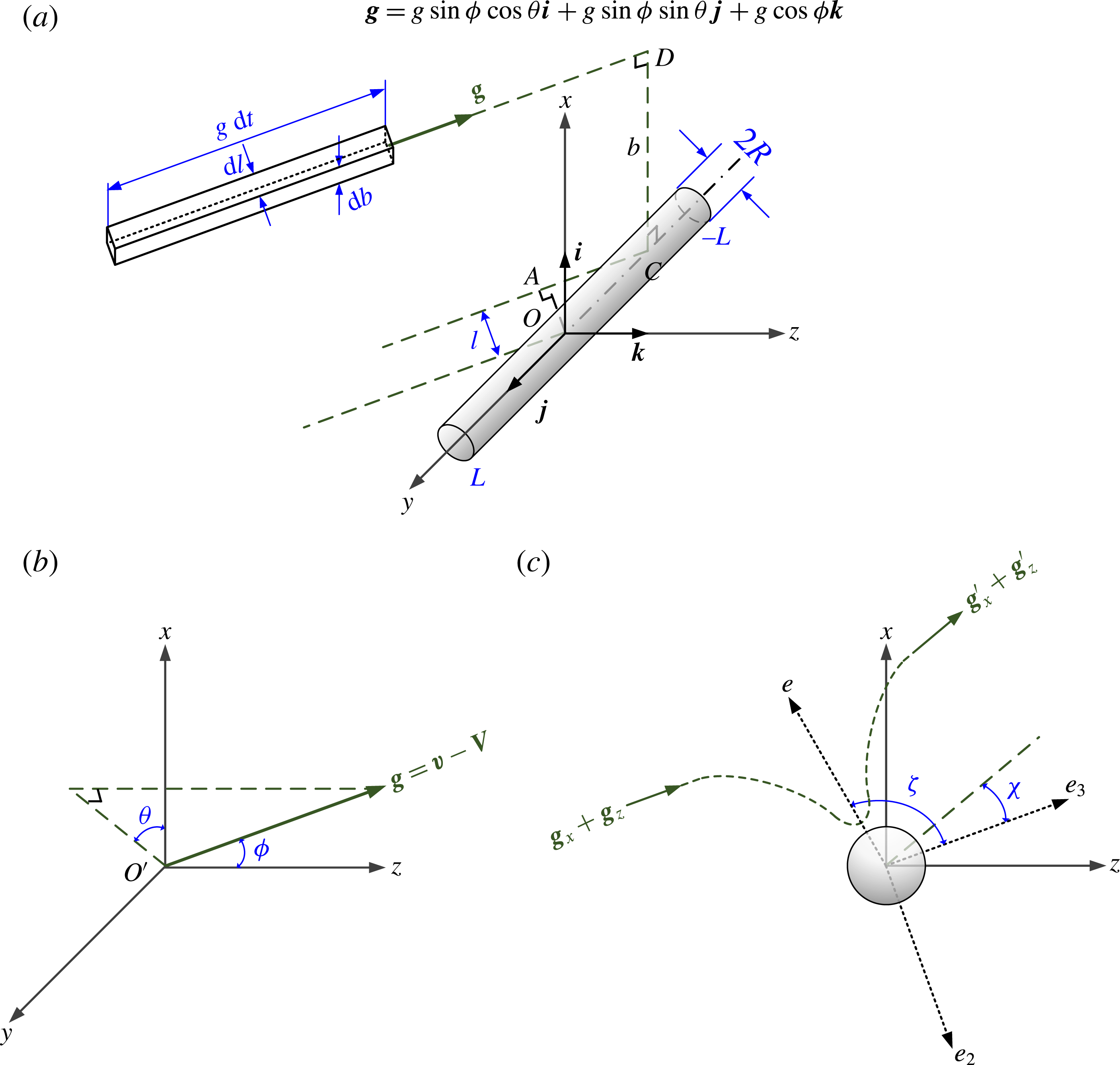
Based on the gas kinetic theory, the cylinder suspended in a rarefied gas undergoes numerous collisions with the surrounding gas molecules. The force is equal to the total momentum transfer to the particle per unit time upon these collisions. The collision model between the cylinder and the gas molecules is shown in figure 2(a). The mean velocity of the cylinder relative to the gas is denoted by
 $\boldsymbol{V}$
. The thermal velocity of the gas molecule is denoted by
 $\boldsymbol{v}$
. The gas molecules travelling in a rectangular element with cross-section
 $\text{d}l\,\text{d}b$
are supposed to collide with the cylinder in a time interval
 $\text{d}t$
, where
 $l$
is the perpendicular distance between the ACD plane and the centre of the cylinder and
 $b$
is the impact parameter. After gas–cylinder collisions, the velocities of the gas molecule and the cylinder are denoted by
 $\boldsymbol{v}^{\prime }$
and
 $\boldsymbol{V}^{\prime }$
, respectively. So, the thermal velocities of the gas molecules with respect to the relative velocities of the cylinder before and after collision are given by
 $\boldsymbol{g}=\boldsymbol{v}-\boldsymbol{V}$
and
 $\boldsymbol{g}^{\prime }=\boldsymbol{v}^{\prime }-\boldsymbol{V}^{\prime }$
. The colatitude and azimuthal angles of
 $\boldsymbol{g}$
are denoted by
 $\unicode[STIX]{x1D719}$
and
 $\unicode[STIX]{x1D703}$
, as shown in figure 2(b). Therefore, the relative velocity vector
 $\boldsymbol{g}$
can be expressed as
 $$\begin{eqnarray}\boldsymbol{g}=g\sin \unicode[STIX]{x1D719}\cos \unicode[STIX]{x1D703}\boldsymbol{i}+g\sin \unicode[STIX]{x1D719}\sin \unicode[STIX]{x1D703}\boldsymbol{j}+g\cos \unicode[STIX]{x1D719}\boldsymbol{k}.\end{eqnarray}$$
(a) Collisions between the gas molecules and the cylinder. (b) Relationship among velocity vectors. (c)
 $x$
–
 $z$
plane projection of the trajectory of the gas molecule.

The number of the gas molecules in the rectangular element in figure 2 at time
 $t$
is given by
 $$\begin{eqnarray}N=gf\,\text{d}l\,\text{d}b\,\text{d}t,\end{eqnarray}$$
and the total momentum carried by these gas molecules is
 $$\begin{eqnarray}\boldsymbol{p}=m_{r}N\boldsymbol{g},\end{eqnarray}$$
where
 $f$
is the velocity distribution function of the gas molecules,
 $m_{r}=m_{g}m_{c}/(m_{g}+m_{c})$
is the reduced mass of a gas molecule with mass
 $m_{g}$
and a cylinder with mass
 $m_{c}$
. In the free molecule regime, the gas molecules reflected by the cylinder surface can usually move for a long distance before colliding with other gas molecules. So, it is reasonable to assume that the velocity distribution of the gas molecules is uninfluenced by the presence of the cylinder. Then, in a shear flow, the velocity distribution function for gas molecules can be given by the second-order approximation of the Chapman–Enskog theory (Chapman & Cowling Reference Chapman and Cowling1970):
 $$\begin{eqnarray}f=f^{(0)}+f^{(1)},\end{eqnarray}$$
where
 $f^{(0)}$
is the Maxwellian velocity distribution for an equilibrium gas
 $$\begin{eqnarray}f^{(0)}=n\left({\displaystyle \frac{h}{\sqrt{\unicode[STIX]{x03C0}}}}\right)^{3}\exp (-h^{2}v^{2}),\end{eqnarray}$$
 $h=\sqrt{m_{r}/(2k_{B}T)}$
,
 $k_{B}$
is the Boltzmann constant,
 $n$
is the number density, and
 $f^{(1)}$
accounts for the perturbation from the equilibrium due to the velocity gradient. For the shear flow shown in figure 1,
 $f^{(1)}$
is given by (Bird, Hirschfelder & Curtiss Reference Bird, Hirschfelder and Curtiss1954; Chapman & Cowling Reference Chapman and Cowling1970; Bird Reference Bird1994)
 $$\begin{eqnarray}f^{(1)}=-f^{(0)}{\displaystyle \frac{5\sqrt{\unicode[STIX]{x03C0}}h^{3}}{4}}v_{X}v_{Y}G,\end{eqnarray}$$
where
 $v_{X}$
and
 $v_{Y}$
are the thermal velocity components in the
 $X$
and
 $Y$
directions.
Following the gas–cylinder collisions, the gas molecules can be scattered either specularly or diffusely. The momentum of the reflected molecules depends on the scattering scenario. Thus, the formulae for the lift force acting on the nanocylinder for the specular scattering model and the diffuse scattering model will be derived separately.
3 Lift force formulae on nanocylinders in the free molecule regime
3.1 Specular scattering
Specular scattering is an ideally elastic collision between the gas molecule and the cylinder, by which the magnitudes of the gas molecule velocity before and after the collision are equal and the incident angle is equal to the reflection angle. For cylinders smaller than a few nanometres in diameter, collisions between the gas molecules and the cylinder can be treated as specular scattering (Liu et al.
Reference Liu, Li and Wang2016a
,Reference Liu, McGivern, Manion and Wang
b
). We assume that the length of the cylinder is much longer than the range of the gas–cylinder interactions, i.e., an infinitely long cylinder is assumed here. Under this assumption, momentum transfer along the cylinder axis (
 $y$
direction) can be neglected; thus, momentum transfer takes place in the
 $x$
–
 $z$
plane (Liu et al.
Reference Liu, Li and Wang2016a
,Reference Liu, McGivern, Manion and Wang
b
; Wang et al.
Reference Wang, Luo and Xia2017). Figure 2(c) presents the
 $x$
–
 $z$
plane projection of the trajectory of a gas molecule which strikes the cylinder with relative velocity
 $\boldsymbol{g}$
and impact parameter
 $b$
. The scattering angle
 $\unicode[STIX]{x1D712}$
is given by
 $$\begin{eqnarray}\unicode[STIX]{x1D712}=\unicode[STIX]{x03C0}-2b\int _{r_{m}}^{\infty }r^{-2}\left[1-{\displaystyle \frac{b^{2}}{r^{2}}}-{\displaystyle \frac{2\unicode[STIX]{x1D6F7}(r)}{m_{r}(g_{x}^{2}+g_{z}^{2})}}\right]^{-1/2}\,\text{d}r,\end{eqnarray}$$
where
 $r$
is the centre-to-axis distance between the gas molecule and the cylinder, and
 $r_{m}$
is the distance of the closest approach. The gas–cylinder interaction potential function
 $\unicode[STIX]{x1D6F7}(r)$
is included in the expression for
 $\unicode[STIX]{x1D712}$
. It is convenient to define a secondary frame, where the unit vector
 $\boldsymbol{e}_{\text{3}}$
is parallel to the incident molecule velocity and
 $\boldsymbol{e}_{2}$
is perpendicular to both the cylinder axis and
 $\boldsymbol{e}_{3}$
, as shown in figure 2(c).
 $\boldsymbol{e}$
is a unit vector normal to the surface of impact.
 $\unicode[STIX]{x1D701}$
is the angle between the molecule incident direction and
 $\boldsymbol{e}$
. The relationship between
 $\unicode[STIX]{x1D701}$
and
 $\unicode[STIX]{x1D712}$
is
 $\unicode[STIX]{x1D701}=(\unicode[STIX]{x1D712}+\unicode[STIX]{x03C0})/2$
. Since
 $\boldsymbol{g}^{\prime }=\boldsymbol{g}_{y}+|\boldsymbol{g}_{x}+\boldsymbol{g}_{z}|(\cos \unicode[STIX]{x1D712}\boldsymbol{e}_{\text{3}}-\sin \unicode[STIX]{x1D712}\boldsymbol{e}_{2})$
, the momentum of the gas molecules with a given impact parameter
 $b$
after collisions is
 $$\begin{eqnarray}\boldsymbol{p}^{\prime }=m_{r}N[\boldsymbol{g}_{y}+|\boldsymbol{g}_{x}+\boldsymbol{g}_{z}|(\cos \unicode[STIX]{x1D712}\boldsymbol{e}_{3}-\sin \unicode[STIX]{x1D712}\boldsymbol{e}_{2})].\end{eqnarray}$$
The net momentum transfer per unit time is
 $$\begin{eqnarray}\text{d}\boldsymbol{F}_{s}={\displaystyle \frac{\boldsymbol{p}-\boldsymbol{p}^{\prime }}{\text{d}t}}=m_{r}N|\boldsymbol{g}_{x}+\boldsymbol{g}_{z}|[(1-\cos \unicode[STIX]{x1D712})\boldsymbol{e}_{3}+\sin \unicode[STIX]{x1D712}\boldsymbol{e}_{2}].\end{eqnarray}$$
The total force on the cylinder can be obtained by integrating (3.3) over the velocity space and incident cross-section. The second term in the square bracket,
 $\sin \unicode[STIX]{x1D712}\boldsymbol{e}_{2}$
, vanishes upon integration over
 $b$
from
 $-\infty$
to
 $\infty$
, due to the symmetry. Thus, the total force acting on the cylinder is
 $$\begin{eqnarray}\boldsymbol{F}_{s}=m_{r}\int _{\boldsymbol{v}}g(f^{(0)}+f^{(1)})(g_{x}\boldsymbol{i}+g_{z}\boldsymbol{k})Q_{s,\bot }\,\text{d}\boldsymbol{v},\end{eqnarray}$$
where
 $Q_{s,\bot }=$
 $Q_{s,\bot }(g)$
is the collision cross-section,
 $$\begin{eqnarray}Q_{s,\bot }=\int _{-\infty }^{\infty }\int _{-L^{^{\prime }}/2}^{L^{^{\prime }}/2}(1-\cos \unicode[STIX]{x1D712})\,\text{d}l\,\text{d}b,\end{eqnarray}$$
the subscript
 $\bot$
denotes that the force is perpendicular to the cylinder axis.
 $L^{\prime }$
is the range where the interaction between the cylinder and gas molecule occurs. For a cylinder with aspect ratio
 $L/(2R)\gg 1$
,
 $L^{\prime }$
approximates to the length of the projection of the cylinder on the plane perpendicular to the direction of
 $\boldsymbol{g}$
,
 $L^{\prime }=L\sqrt{\cos ^{2}\unicode[STIX]{x1D719}+\cos ^{2}\unicode[STIX]{x1D703}\sin ^{2}\unicode[STIX]{x1D719}}$
. The right-hand side of (3.4) consists of two contributions: a drag force involving
 $f^{(0)}$
, which is given by Liu et al. (Reference Liu, Li and Wang2016a
,Reference Liu, McGivern, Manion and Wang
b
), and a lift force involving
 $f^{(1)}$
. The lift force in the integral form is
 $$\begin{eqnarray}\boldsymbol{F}_{L,s}=m_{r}\int _{\boldsymbol{v}}gf^{(1)}(g_{x}\boldsymbol{i}+g_{z}\boldsymbol{k})Q_{s,\bot }\,\text{d}\boldsymbol{v}.\end{eqnarray}$$
To calculate the integration in (3.6), it is convenient to transform the thermal velocity components from the global coordinate system
 $\{XYZ\}$
to the particle coordinate system
 $\{xyz\}$
by
 $[v_{x},v_{y},v_{z}]^{\text{T}}=\unicode[STIX]{x1D614}^{-1}[v_{X},v_{Y},v_{Z}]^{\text{T}}$
. As a result, the velocity distribution function in the
 $\{xyz\}$
system is
 $$\begin{eqnarray}\displaystyle f^{(1)} & = & \displaystyle -f^{(0)}{\displaystyle \frac{5\sqrt{\unicode[STIX]{x03C0}}h^{3}}{4}}\big[-v_{x}^{2}\sin \unicode[STIX]{x1D6FC}\cos \unicode[STIX]{x1D6FC}\cos \unicode[STIX]{x1D6FD}+v_{x}v_{y}(\cos ^{2}\unicode[STIX]{x1D6FC}-\sin ^{2}\unicode[STIX]{x1D6FC})\cos \unicode[STIX]{x1D6FD}\nonumber\\ \displaystyle & & \displaystyle +\,v_{y}^{2}\sin \unicode[STIX]{x1D6FC}\cos \unicode[STIX]{x1D6FC}\cos \unicode[STIX]{x1D6FD}+v_{x}v_{z}\sin \unicode[STIX]{x1D6FC}\sin \unicode[STIX]{x1D6FD}-v_{y}v_{z}\cos \unicode[STIX]{x1D6FC}\sin \unicode[STIX]{x1D6FD}\big]G,\end{eqnarray}$$
where
 $v_{x}$
,
 $v_{y}$
,
 $v_{z}$
can be written as
 $$\begin{eqnarray}\displaystyle & \displaystyle v_{x}=g_{x}+V_{x}=g\sin \unicode[STIX]{x1D719}\cos \unicode[STIX]{x1D703}-U_{0}\cos \unicode[STIX]{x1D6FC}\cos \unicode[STIX]{x1D6FD}, & \displaystyle\end{eqnarray}$$
 $$\begin{eqnarray}\displaystyle & \displaystyle v_{y}=g_{y}+V_{y}=g\sin \unicode[STIX]{x1D719}\sin \unicode[STIX]{x1D703}-U_{0}\sin \unicode[STIX]{x1D6FC}\cos \unicode[STIX]{x1D6FD}, & \displaystyle\end{eqnarray}$$
 $$\begin{eqnarray}\displaystyle & \displaystyle v_{z}=g_{z}+V_{z}=g\cos \unicode[STIX]{x1D719}+U_{0}\sin \unicode[STIX]{x1D6FD}. & \displaystyle\end{eqnarray}$$
In general, the magnitude of the molecule thermal velocity
 $\boldsymbol{v}$
is much larger than that of the cylinder velocity
 $\boldsymbol{V}$
, so that
 $f^{(0)}$
can be simplified by expanding the exponential term
 $\exp (-h^{2}v^{2})$
as a power series and neglecting the higher-order terms,
 $$\begin{eqnarray}\displaystyle f^{(0)} & {\approx} & \displaystyle n\left({\displaystyle \frac{h}{\sqrt{\unicode[STIX]{x03C0}}}}\right)^{3}\exp (-h^{2}g^{2})\big[1+2h^{2}gU_{o}\big(\sin \unicode[STIX]{x1D719}\cos \unicode[STIX]{x1D703}\cos \unicode[STIX]{x1D6FC}\cos \unicode[STIX]{x1D6FD}\nonumber\\ \displaystyle & & \displaystyle +\sin \unicode[STIX]{x1D719}\sin \unicode[STIX]{x1D703}\sin \unicode[STIX]{x1D6FC}\cos \unicode[STIX]{x1D6FD}-\cos \unicode[STIX]{x1D719}\sin \unicode[STIX]{x1D6FD}\big)\big].\end{eqnarray}$$
Moreover,
 $\text{d}\boldsymbol{v}\approx \text{d}\boldsymbol{g}$
. Combining (3.6)–(3.11), we obtain the components of
 $\boldsymbol{F}_{L,s}$
in the
 $\{xyz\}$
coordinate system
 $$\begin{eqnarray}\displaystyle \boldsymbol{F}_{L,s,x} & = & \displaystyle {\displaystyle \frac{5\unicode[STIX]{x1D70C}\unicode[STIX]{x1D706}GU_{0}RL}{2\unicode[STIX]{x03C0}}}\big[(6\unicode[STIX]{x1D6FA}_{s,\bot ,1}^{(1,2)\ast }-18\unicode[STIX]{x1D6FA}_{s,\bot ,3}^{(1,2)\ast })\sin \unicode[STIX]{x1D6FC}\cos ^{2}\unicode[STIX]{x1D6FC}\cos ^{2}\unicode[STIX]{x1D6FD}\nonumber\\ \displaystyle & & \displaystyle +\,(6\unicode[STIX]{x1D6FA}_{s,\bot ,3}^{(1,2)\ast }-\unicode[STIX]{x1D6FA}_{s,\bot ,1}^{(1,1)\ast })\sin \unicode[STIX]{x1D6FC}\cos ^{2}\unicode[STIX]{x1D6FD}+(6\unicode[STIX]{x1D6FA}_{s,\bot ,2}^{(1,2)\ast }-\unicode[STIX]{x1D6FA}_{s,\bot ,1}^{(1,1)\ast })\sin \unicode[STIX]{x1D6FC}\sin ^{2}\unicode[STIX]{x1D6FD}\big]\boldsymbol{i},\qquad\end{eqnarray}$$
 $$\begin{eqnarray}\displaystyle \boldsymbol{F}_{L,s,y} & = & \displaystyle 0,\end{eqnarray}$$
 $$\begin{eqnarray}\displaystyle \boldsymbol{F}_{L,s,z} & = & \displaystyle {\displaystyle \frac{5\unicode[STIX]{x1D70C}\unicode[STIX]{x1D706}GU_{0}RL}{2\unicode[STIX]{x03C0}}}(-12\unicode[STIX]{x1D6FA}_{s,\bot ,2}^{(1,2)\ast }+12\unicode[STIX]{x1D6FA}_{s,\bot ,4}^{(1,2)\ast })\sin \unicode[STIX]{x1D6FC}\cos \unicode[STIX]{x1D6FC}\sin \unicode[STIX]{x1D6FD}\cos \unicode[STIX]{x1D6FD}\boldsymbol{k},\end{eqnarray}$$
where
 $$\begin{eqnarray}\displaystyle & \displaystyle \unicode[STIX]{x1D6FA}_{s,\bot ,l}^{(1,1)\ast }={\displaystyle \frac{1}{2RL}}\int _{0}^{\infty }\int _{0}^{2\unicode[STIX]{x03C0}}\int _{0}^{\unicode[STIX]{x03C0}}\unicode[STIX]{x1D709}^{5}\exp (-\unicode[STIX]{x1D709}^{2})Q_{s,\bot }\unicode[STIX]{x1D6E4}_{l}\,\text{d}\unicode[STIX]{x1D719}\,\text{d}\unicode[STIX]{x1D703}\,\text{d}\unicode[STIX]{x1D709},\quad l=1, & \displaystyle\end{eqnarray}$$
 $$\begin{eqnarray}\displaystyle & \displaystyle \unicode[STIX]{x1D6FA}_{s,\bot ,m}^{(1,2)\ast }={\displaystyle \frac{1}{6RL}}\int _{0}^{\infty }\int _{0}^{2\unicode[STIX]{x03C0}}\int _{0}^{\unicode[STIX]{x03C0}}\unicode[STIX]{x1D709}^{7}\exp (-\unicode[STIX]{x1D709}^{2})Q_{s,\bot }\unicode[STIX]{x1D6EC}_{m}\,\text{d}\unicode[STIX]{x1D719}\,\text{d}\unicode[STIX]{x1D703}\,\text{d}\unicode[STIX]{x1D709},\quad m=1,2,3,4, & \displaystyle\end{eqnarray}$$
are the defined reduced collision integrals with
 $\unicode[STIX]{x1D709}=gh$
.
 $\unicode[STIX]{x1D6E4}_{l}$
and
 $\unicode[STIX]{x1D6EC}_{m}$
are trigonometric functions of
 $\unicode[STIX]{x1D719}$
and
 $\unicode[STIX]{x1D703}$
(see appendix A). The lift forces in the global coordinate system can be obtained by the transformation matrix,
 $$\begin{eqnarray}\left[\begin{array}{@{}c@{}}\boldsymbol{F}_{L,X}\\ \boldsymbol{F}_{L,Y}\\ \boldsymbol{F}_{L,Z}\\ \end{array}\right]=\left[\begin{array}{@{}ccc@{}}\cos \unicode[STIX]{x1D6FC}\cos \unicode[STIX]{x1D6FD} & \sin \unicode[STIX]{x1D6FC}\cos \unicode[STIX]{x1D6FD} & -\sin \unicode[STIX]{x1D6FD}\\ -\sin \unicode[STIX]{x1D6FC} & \cos \unicode[STIX]{x1D6FC} & 0\\ \cos \unicode[STIX]{x1D6FC}\sin \unicode[STIX]{x1D6FD} & \sin \unicode[STIX]{x1D6FC}\sin \unicode[STIX]{x1D6FD} & \cos \unicode[STIX]{x1D6FD}\\ \end{array}\right]\left[\begin{array}{@{}c@{}}\boldsymbol{F}_{L,x}\\ \boldsymbol{ F}_{L,y}\\ \boldsymbol{ F}_{L,z}\\ \end{array}\right].\end{eqnarray}$$
Therefore, we obtain the lift force on the cylinder for the specular scattering case as
 $$\begin{eqnarray}\displaystyle \boldsymbol{F}_{L,s,X} & = & \displaystyle {\displaystyle \frac{5\unicode[STIX]{x1D70C}\unicode[STIX]{x1D706}GU_{0}RL}{2\unicode[STIX]{x03C0}}}\big[(6\unicode[STIX]{x1D6FA}_{s,\bot ,1}^{(1,2)\ast }-18\unicode[STIX]{x1D6FA}_{s,\bot ,3}^{(1,2)\ast })\sin \unicode[STIX]{x1D6FC}\cos ^{3}\unicode[STIX]{x1D6FC}\cos ^{3}\unicode[STIX]{x1D6FD}\nonumber\\ \displaystyle & & \displaystyle +\,(6\unicode[STIX]{x1D6FA}_{s,\bot ,3}^{(1,2)\ast }-\unicode[STIX]{x1D6FA}_{s,\bot ,1}^{(1,1)\ast })\sin \unicode[STIX]{x1D6FC}\cos \unicode[STIX]{x1D6FC}\cos \unicode[STIX]{x1D6FD}\nonumber\\ \displaystyle & & \displaystyle +\,(18\unicode[STIX]{x1D6FA}_{s,\bot ,2}^{(1,2)\ast }-6\unicode[STIX]{x1D6FA}_{s,\bot ,3}^{(1,2)\ast }-12\unicode[STIX]{x1D6FA}_{s,\bot ,4}^{(1,2)\ast })\sin \unicode[STIX]{x1D6FC}\cos \unicode[STIX]{x1D6FC}\sin ^{2}\unicode[STIX]{x1D6FD}\cos \unicode[STIX]{x1D6FD}\big]\boldsymbol{I},\end{eqnarray}$$
 $$\begin{eqnarray}\displaystyle \boldsymbol{F}_{L,s,Y} & = & \displaystyle {\displaystyle \frac{5\unicode[STIX]{x1D70C}\unicode[STIX]{x1D706}GU_{0}RL}{2\unicode[STIX]{x03C0}}}\big[(-6\unicode[STIX]{x1D6FA}_{s,\bot ,1}^{(1,2)\ast }+18\unicode[STIX]{x1D6FA}_{s,\bot ,3}^{(1,2)\ast })\cos ^{2}\unicode[STIX]{x1D6FC}\cos ^{2}\unicode[STIX]{x1D6FE}\nonumber\\ \displaystyle & & \displaystyle +\,(-6\unicode[STIX]{x1D6FA}_{s,\bot ,3}^{(1,2)\ast }+\unicode[STIX]{x1D6FA}_{s,\bot ,1}^{(1,1)\ast })\cos ^{2}\unicode[STIX]{x1D6FE}+(-6\unicode[STIX]{x1D6FA}_{s,\bot ,2}^{(1,2)\ast }+\unicode[STIX]{x1D6FA}_{s,\bot ,1}^{(1,1)\ast })(\sin ^{2}\unicode[STIX]{x1D6FC}-\cos ^{2}\unicode[STIX]{x1D6FE})\big]\boldsymbol{J},\qquad \nonumber\\ \displaystyle & & \displaystyle\end{eqnarray}$$
 $$\begin{eqnarray}\displaystyle \boldsymbol{F}_{L,s,Z} & = & \displaystyle {\displaystyle \frac{5\unicode[STIX]{x1D70C}\unicode[STIX]{x1D706}GU_{0}RL}{2\unicode[STIX]{x03C0}}}\big[(18\unicode[STIX]{x1D6FA}_{s,\bot ,3}^{(1,2)\ast }-6\unicode[STIX]{x1D6FA}_{s,\bot ,1}^{(1,2)\ast })\sin ^{3}\unicode[STIX]{x1D6FC}\cos \unicode[STIX]{x1D6FC}\sin \unicode[STIX]{x1D6FD}\cos ^{2}\unicode[STIX]{x1D6FD}\nonumber\\ \displaystyle & & \displaystyle +\,(6\unicode[STIX]{x1D6FA}_{s,\bot ,2}^{(1,2)\ast }-\unicode[STIX]{x1D6FA}_{s,\bot ,1}^{(1,1)\ast })\sin \unicode[STIX]{x1D6FC}\cos \unicode[STIX]{x1D6FC}\sin \unicode[STIX]{x1D6FD}\nonumber\\ \displaystyle & & \displaystyle +\,(6\unicode[STIX]{x1D6FA}_{s,\bot ,1}^{(1,2)\ast }-18\unicode[STIX]{x1D6FA}_{s,\bot ,2}^{(1,2)\ast }-12\unicode[STIX]{x1D6FA}_{s,\bot ,3}^{(1,2)\ast }+12\unicode[STIX]{x1D6FA}_{s,\bot ,4}^{(1,2)\ast })\sin \unicode[STIX]{x1D6FC}\cos \unicode[STIX]{x1D6FC}\sin ^{3}\unicode[STIX]{x1D6FD}\big]\boldsymbol{K}.\end{eqnarray}$$
The reduced collision integrals in the above equations depend on the potential energy of gas–cylinder interactions. Note that there exist force components in the
 $X$
and
 $Z$
directions, which are due to the pitching effect of the cylinder. The lift force is usually defined in the
 $Y$
direction (parallel to the flow gradient
 $\boldsymbol{G}$
). The force components in the
 $X$
and
 $Z$
directions can be considered as transverse forces of the shear lift. Under a uniformly random distribution of the cylinder orientation, the transverse forces vanish, as shown in § 3.4.
For microsized cylinders, the van der Waals interaction becomes insignificant and the rigid-body assumption is valid, for which the collision integrals can be easily obtained (see (A 2) in appendix A). Substituting these collision integral values of rigid-body collisions into (3.18)–(3.20), the force components read
 $$\begin{eqnarray}\displaystyle & \displaystyle \boldsymbol{F}_{L,s,X}={\displaystyle \frac{15\unicode[STIX]{x03C0}\unicode[STIX]{x1D70C}\unicode[STIX]{x1D706}GV_{o}RL}{16}}(\sin \unicode[STIX]{x1D6FC}\cos ^{3}\unicode[STIX]{x1D6FC}\cos ^{3}\unicode[STIX]{x1D6FD}+\sin \unicode[STIX]{x1D6FC}\cos \unicode[STIX]{x1D6FC}\sin ^{2}\unicode[STIX]{x1D6FD}\cos \unicode[STIX]{x1D6FD})\boldsymbol{I}, & \displaystyle\end{eqnarray}$$
 $$\begin{eqnarray}\displaystyle & \displaystyle \boldsymbol{F}_{L,s,Y}=-{\displaystyle \frac{5\unicode[STIX]{x03C0}\unicode[STIX]{x1D70C}\unicode[STIX]{x1D706}GV_{o}RL}{16}}(3\cos ^{2}\unicode[STIX]{x1D6FC}\cos ^{2}\unicode[STIX]{x1D6FE}+\sin ^{2}\unicode[STIX]{x1D6FC}-\cos ^{2}\unicode[STIX]{x1D6FE})\boldsymbol{J}, & \displaystyle\end{eqnarray}$$
 $$\begin{eqnarray}\displaystyle & \displaystyle \boldsymbol{F}_{L,s,Z}=-{\displaystyle \frac{5\unicode[STIX]{x03C0}\unicode[STIX]{x1D70C}\unicode[STIX]{x1D706}GV_{o}RL}{16}}(3\sin ^{3}\unicode[STIX]{x1D6FC}\cos \unicode[STIX]{x1D6FC}\sin \unicode[STIX]{x1D6FD}\cos ^{2}\unicode[STIX]{x1D6FD}-\sin \unicode[STIX]{x1D6FC}\cos \unicode[STIX]{x1D6FC}\sin \unicode[STIX]{x1D6FD})\boldsymbol{K}. & \displaystyle\end{eqnarray}$$
Equation (3.22) in the
 $Y$
direction is consistent with (1.1) in the case of specular scattering (
 $\unicode[STIX]{x1D70E}_{\unicode[STIX]{x1D70F}}=\unicode[STIX]{x1D70E}_{p}=0$
). Equations (3.21) and (3.23) are the transverse forces for specular scattering in the limit of rigid-body collisions.
3.2 Diffuse scattering
The diffuse scattering originates from trapping of the gas molecule on the surface (Li & Wang Reference Li and Wang2005), which is the dominant scattering scenario for cylinders with large radius. Because of thermal fluctuations of the cylinder, the absorbed molecules can be re-emitted with a Maxwellian velocity distribution corresponding to the cylinder temperature (assumed to be equal to the gas temperature) (Li & Wang Reference Li and Wang2004),
 $$\begin{eqnarray}f^{\prime }=cg(f^{(0)}+f^{(1)})\exp \left(-{\displaystyle \frac{m_{r}{g^{\prime }}^{2}}{2k_{B}T}}\right),\end{eqnarray}$$
where
 $c$
is a constant and its value may be determined by mass conservation as
 $c=m_{r}k_{B}T^{2}/(2\unicode[STIX]{x03C0})$
. Since the net momentum transfer is zero in the direction parallel to the surface, the momentum of the reflected gas molecule can be written as
 $$\begin{eqnarray}\boldsymbol{p}^{\prime }=\sqrt{{\displaystyle \frac{\unicode[STIX]{x03C0}m_{r}k_{B}T}{2}}}g(f^{(0)}+f^{(1)})\,\text{d}l\,\text{d}b\,\text{d}t\boldsymbol{e}.\end{eqnarray}$$
By using the relationship among unit vectors
 $\boldsymbol{e}$
,
 $\boldsymbol{e}_{2}$
and
 $\boldsymbol{e}_{3}$
, the differential force can be written as
 $$\begin{eqnarray}\text{d}\boldsymbol{F}_{d}={\displaystyle \frac{\boldsymbol{p}-\boldsymbol{p}^{\prime }}{\text{d}t}}=m_{r}g(f^{(0)}+f^{(1)})\left[\boldsymbol{g}-\sqrt{{\displaystyle \frac{\unicode[STIX]{x03C0}k_{B}T}{2m_{r}}}}(\cos \unicode[STIX]{x1D701}\boldsymbol{e}_{3}-\sin \unicode[STIX]{x1D701}\boldsymbol{e}_{2})\right]\,\text{d}l\,\text{d}b.\end{eqnarray}$$
Again, the component in the
 $\boldsymbol{e}_{2}$
direction vanishes upon integration over
 $b$
due to the symmetry. Therefore the total force acting on the cylinder for diffuse scattering is obtained as
 $$\begin{eqnarray}\boldsymbol{F}_{d}=\int _{\boldsymbol{v}}\int _{-\infty }^{\infty }\int _{-L^{\prime }/2}^{L^{\prime }/2}m_{r}g(f^{(0)}+f^{(1)})\left[\boldsymbol{g}+\sqrt{{\displaystyle \frac{\unicode[STIX]{x03C0}k_{B}T}{2m_{r}}}}\sin \left({\displaystyle \frac{\unicode[STIX]{x1D712}}{2}}\right)\boldsymbol{e}_{3}\right]\,\text{d}l\,\text{d}b\,\text{d}\boldsymbol{v}.\end{eqnarray}$$
Here, the integration of the
 $f^{(0)}$
term is the drag force (Liu et al.
Reference Liu, Li and Wang2016a
,Reference Liu, McGivern, Manion and Wang
b
). The lift force is given by the integration of
 $f^{(1)}$
,
 $$\begin{eqnarray}\boldsymbol{F}_{L,d}=\int _{\boldsymbol{v}}\int _{-\infty }^{\infty }\int _{-L^{\prime }/2}^{L^{\prime }/2}m_{r}gf^{(1)}\left[\boldsymbol{g}+\sqrt{{\displaystyle \frac{\unicode[STIX]{x03C0}k_{B}T}{2m_{r}}}}\sin \left({\displaystyle \frac{\unicode[STIX]{x1D712}}{2}}\right)\boldsymbol{e}_{3}\right]\,\text{d}l\,\text{d}b\,\text{d}\boldsymbol{v},\end{eqnarray}$$
which can be decomposed as
 $$\begin{eqnarray}\boldsymbol{F}_{L,d}=m_{r}\left[\int _{\boldsymbol{v}}gf^{(1)}g_{x}\boldsymbol{i}Q_{d,\bot }\,\text{d}\boldsymbol{v}+\int _{\boldsymbol{v}}gf^{(1)}g_{y}\,\boldsymbol{j}Q_{d,\Vert }\,\text{d}\boldsymbol{v}+\int _{\boldsymbol{v}}gf^{(1)}g_{z}Q_{d,\bot }\boldsymbol{k}\,\text{d}\boldsymbol{v}\right].\end{eqnarray}$$
Here,
 $Q_{d,\bot }$
and
 $Q_{d,\Vert }$
are collision cross-sections for diffuse scattering
 $$\begin{eqnarray}\displaystyle Q_{d,\bot } & = & \displaystyle 2\int _{0}^{b_{0}}\int _{-L^{\prime }/2}^{L^{\prime }/2}\left\{1+\left[{\displaystyle \frac{\unicode[STIX]{x03C0}k_{B}T}{2m_{r}(g_{z}^{2}+g_{x}^{2})}}\right]^{1/2}\sin (\unicode[STIX]{x1D712}/2)\right\}\,\text{d}l\,\text{d}b\nonumber\\ \displaystyle & & \displaystyle +\,2\int _{b_{0}}^{\infty }\int _{-L^{\prime }/2}^{L^{\prime }/2}(1-\cos \unicode[STIX]{x1D712})\,\text{d}l\,\text{d}b,\end{eqnarray}$$
 $$\begin{eqnarray}\displaystyle Q_{d,\Vert } & = & \displaystyle 2b_{0}L^{\prime },\end{eqnarray}$$
and the subscript
 $\Vert$
denotes the force parallel to the cylinder axis. Here,
 $b_{\text{0}}$
is the critical impact factor and
 $b=b_{\text{0}}$
corresponds to the orbital scattering (
 $\unicode[STIX]{x1D712}\rightarrow \infty$
). For
 $b<b_{0}$
, the gas molecules can physically collide with the cylinder (
 $-\infty <\unicode[STIX]{x1D712}\leqslant \unicode[STIX]{x03C0}$
) and diffuse scattering takes place, whereas for
 $b>b_{0}$
, the gas molecules undergo grazing scattering, and the gas–cylinder collision is specular. By a similar method to that used for specular scattering, equation (3.29) can be simplified to
 $$\begin{eqnarray}\displaystyle \boldsymbol{F}_{L,d,x} & = & \displaystyle {\displaystyle \frac{5\unicode[STIX]{x1D70C}\unicode[STIX]{x1D706}GU_{0}RL}{2\unicode[STIX]{x03C0}}}\left[(6\unicode[STIX]{x1D6FA}_{d,\bot ,1}^{(1,2)\ast }-18\unicode[STIX]{x1D6FA}_{d,\bot ,3}^{(1,2)\ast })\sin \unicode[STIX]{x1D6FC}\cos ^{2}\unicode[STIX]{x1D6FC}\right.\cos ^{2}\unicode[STIX]{x1D6FD}\nonumber\\ \displaystyle & & \displaystyle \left.+\,(6\unicode[STIX]{x1D6FA}_{d,\bot ,3}^{(1,2)\ast }-\unicode[STIX]{x1D6FA}_{d,\bot ,1}^{(1,1)\ast })\sin \unicode[STIX]{x1D6FC}\cos ^{2}\unicode[STIX]{x1D6FD}+(6\unicode[STIX]{x1D6FA}_{d,\bot ,2}^{(1,2)\ast }-\unicode[STIX]{x1D6FA}_{d,\bot ,1}^{(1,1)\ast })\sin \unicode[STIX]{x1D6FC}\sin ^{2}\unicode[STIX]{x1D6FD}\right]\!\boldsymbol{i},\end{eqnarray}$$
 $$\begin{eqnarray}\displaystyle \boldsymbol{F}_{L,d,y} & = & \displaystyle {\displaystyle \frac{5\unicode[STIX]{x1D70C}\unicode[STIX]{x1D706}GU_{0}RL}{2\unicode[STIX]{x03C0}}}\left[(18\unicode[STIX]{x1D6FA}_{d,\Vert ,1}^{(1,2)\ast }-6\unicode[STIX]{x1D6FA}_{d,\Vert ,2}^{(1,2)\ast })\sin ^{2}\unicode[STIX]{x1D6FC}\cos \unicode[STIX]{x1D6FC}\cos ^{2}\unicode[STIX]{x1D6FD}\right.\nonumber\\ \displaystyle & & \displaystyle \left.+\,(-6\unicode[STIX]{x1D6FA}_{d,\Vert ,1}^{(1,2)\ast }+\unicode[STIX]{x1D6FA}_{d,\Vert ,1}^{(1,1)\ast })\cos \unicode[STIX]{x1D6FC}\cos ^{2}\unicode[STIX]{x1D6FD}+(-6\unicode[STIX]{x1D6FA}_{d,\Vert ,3}^{(1,2)\ast }+\unicode[STIX]{x1D6FA}_{d,\Vert ,1}^{(1,1)\ast })\cos \unicode[STIX]{x1D6FC}\sin ^{2}\unicode[STIX]{x1D6FD}\right]\boldsymbol{j},\nonumber\\ \displaystyle & & \displaystyle\end{eqnarray}$$
 $$\begin{eqnarray}\displaystyle \boldsymbol{F}_{L,d,z} & = & \displaystyle {\displaystyle \frac{5\unicode[STIX]{x1D70C}\unicode[STIX]{x1D706}GU_{0}RL}{2\unicode[STIX]{x03C0}}}(-12\unicode[STIX]{x1D6FA}_{d,\bot ,2}^{(1,2)\ast }+12\unicode[STIX]{x1D6FA}_{d,\bot ,4}^{(1,2)\ast })\sin \unicode[STIX]{x1D6FC}\cos \unicode[STIX]{x1D6FC}\sin \unicode[STIX]{x1D6FD}\cos \unicode[STIX]{x1D6FD}\boldsymbol{k},\end{eqnarray}$$
where
 $$\begin{eqnarray}\displaystyle & \displaystyle \unicode[STIX]{x1D6FA}_{d,\bot ,l}^{(1,1)\ast }={\displaystyle \frac{1}{2RL}}\int _{0}^{\infty }\int _{0}^{2\unicode[STIX]{x03C0}}\int _{0}^{\unicode[STIX]{x03C0}}\unicode[STIX]{x1D709}^{5}\exp (-\unicode[STIX]{x1D709}^{2})Q_{d,\bot }\unicode[STIX]{x1D6E4}_{l}\,\text{d}\unicode[STIX]{x1D719}\,\text{d}\unicode[STIX]{x1D703}\,\text{d}\unicode[STIX]{x1D709},\quad l=1,\qquad & \displaystyle\end{eqnarray}$$
 $$\begin{eqnarray}\displaystyle & \displaystyle \unicode[STIX]{x1D6FA}_{d,\bot ,m}^{(1,2)\ast }={\displaystyle \frac{1}{6RL}}\int _{0}^{\infty }\int _{0}^{2\unicode[STIX]{x03C0}}\int _{0}^{\unicode[STIX]{x03C0}}\unicode[STIX]{x1D709}^{7}\exp (-\unicode[STIX]{x1D709}^{2})Q_{d,\bot }\unicode[STIX]{x1D6EC}_{m}\,\text{d}\unicode[STIX]{x1D719}\,\text{d}\unicode[STIX]{x1D703}\,\text{d}\unicode[STIX]{x1D709},\quad m=1,2,3,4,\qquad & \displaystyle\end{eqnarray}$$
 $$\begin{eqnarray}\displaystyle & \displaystyle \unicode[STIX]{x1D6FA}_{d,\Vert ,n}^{(1,1)\ast }={\displaystyle \frac{1}{2RL}}\int _{0}^{\infty }\int _{0}^{2\unicode[STIX]{x03C0}}\int _{0}^{\unicode[STIX]{x03C0}}\unicode[STIX]{x1D709}^{5}\exp (-\unicode[STIX]{x1D709}^{2})Q_{d,\Vert }\unicode[STIX]{x1D6F1}_{n}\,\text{d}\unicode[STIX]{x1D719}\,\text{d}\unicode[STIX]{x1D703}\,\text{d}\unicode[STIX]{x1D709},\quad n=1,\qquad & \displaystyle\end{eqnarray}$$
 $$\begin{eqnarray}\displaystyle & \displaystyle \unicode[STIX]{x1D6FA}_{d,\Vert ,q}^{(1,2)\ast }={\displaystyle \frac{1}{6RL}}\int _{0}^{\infty }\int _{0}^{2\unicode[STIX]{x03C0}}\int _{0}^{\unicode[STIX]{x03C0}}\unicode[STIX]{x1D709}^{7}\exp (-\unicode[STIX]{x1D709}^{2})Q_{d,\Vert }\unicode[STIX]{x1D6F9}_{q}\,\text{d}\unicode[STIX]{x1D719}\,\text{d}\unicode[STIX]{x1D703}\,\text{d}\unicode[STIX]{x1D709},\quad q=1,2,3,\qquad & \displaystyle\end{eqnarray}$$
are the reduced collision integrals for diffuse scattering. The expressions of
 $\unicode[STIX]{x1D6F1}_{n}$
and
 $\unicode[STIX]{x1D6F9}_{q}$
are given in (A 1) in appendix A. Then, by using the transformation matrix, the lift force components in the global coordinate system can be written as
 $$\begin{eqnarray}\displaystyle \boldsymbol{F}_{L,d,X} & = & \displaystyle {\displaystyle \frac{5\unicode[STIX]{x1D70C}\unicode[STIX]{x1D706}GU_{0}RL}{2\unicode[STIX]{x03C0}}}\left[(6\unicode[STIX]{x1D6FA}_{d,\bot ,1}^{(1,2)\ast }-18\unicode[STIX]{x1D6FA}_{d,\bot ,3}^{(1,2)\ast }-18\unicode[STIX]{x1D6FA}_{d,\Vert ,1}^{(1,2)\ast }+6\unicode[STIX]{x1D6FA}_{d,\Vert ,2}^{(1,2)\ast })\sin \unicode[STIX]{x1D6FC}\cos ^{3}\unicode[STIX]{x1D6FC}\right.\cos ^{3}\unicode[STIX]{x1D6FD}\nonumber\\ \displaystyle & & \displaystyle +\,(6\unicode[STIX]{x1D6FA}_{d,\bot ,3}^{(1,2)\ast }-\unicode[STIX]{x1D6FA}_{d,\bot ,1}^{(1,1)\ast }+12\unicode[STIX]{x1D6FA}_{d,\Vert ,1}^{(1,2)\ast }-6\unicode[STIX]{x1D6FA}_{d,\Vert ,2}^{(1,2)\ast }+\unicode[STIX]{x1D6FA}_{d,\Vert ,1}^{(1,1)\ast })\sin \unicode[STIX]{x1D6FC}\cos \unicode[STIX]{x1D6FC}\cos \unicode[STIX]{x1D6FD}\nonumber\\ \displaystyle & & \displaystyle +\,(18\unicode[STIX]{x1D6FA}_{d,\bot ,2}^{(1,2)\ast }-6\unicode[STIX]{x1D6FA}_{d,\bot ,3}^{(1,2)\ast }-12\unicode[STIX]{x1D6FA}_{d,\bot ,4}^{(1,2)\ast }-12\unicode[STIX]{x1D6FA}_{d,\Vert ,1}^{(1,2)\ast }+6\unicode[STIX]{x1D6FA}_{d,\Vert ,2}^{(1,2)\ast }-6\unicode[STIX]{x1D6FA}_{d,\Vert ,3}^{(1,2)\ast })\nonumber\\ \displaystyle & & \displaystyle \left.\times \,\sin \unicode[STIX]{x1D6FC}\cos \unicode[STIX]{x1D6FC}\sin ^{2}\unicode[STIX]{x1D6FD}\cos \unicode[STIX]{x1D6FD}\vphantom{6\unicode[STIX]{x1D6FA}_{d,\bot ,1}^{(1,2)\ast }}\right]\boldsymbol{I},\end{eqnarray}$$
 $$\begin{eqnarray}\displaystyle \boldsymbol{F}_{L,d,Y} & = & \displaystyle {\displaystyle \frac{5\unicode[STIX]{x1D70C}\unicode[STIX]{x1D706}GU_{0}RL}{2\unicode[STIX]{x03C0}}}\left[(-6\unicode[STIX]{x1D6FA}_{d,\bot ,1}^{(1,2)\ast }+18\unicode[STIX]{x1D6FA}_{d,\bot ,3}^{(1,2)\ast }+18\unicode[STIX]{x1D6FA}_{d,\Vert ,1}^{(1,2)\ast }-6\unicode[STIX]{x1D6FA}_{d,\Vert ,2}^{(1,2)\ast })\cos ^{2}\unicode[STIX]{x1D6FC}\right.\cos ^{2}\unicode[STIX]{x1D6FE}\nonumber\\ \displaystyle & & \displaystyle +\,(-6\unicode[STIX]{x1D6FA}_{d,\bot ,2}^{(1,2)\ast }+\unicode[STIX]{x1D6FA}_{d,\bot ,1}^{(1,1)\ast })(\sin ^{2}\unicode[STIX]{x1D6FC}-\cos ^{2}\unicode[STIX]{x1D6FE})+(-6\unicode[STIX]{x1D6FA}_{d,\bot ,3}^{(1,2)\ast }+\unicode[STIX]{x1D6FA}_{d,\bot ,1}^{(1,1)\ast })\cos ^{2}\unicode[STIX]{x1D6FE}\nonumber\\ \displaystyle & & \displaystyle \left.+\,(-6\unicode[STIX]{x1D6FA}_{d,\Vert ,1}^{(1,2)\ast }+\unicode[STIX]{x1D6FA}_{d,\Vert ,1}^{(1,1)\ast })\cos ^{2}\unicode[STIX]{x1D6FC}\cos ^{2}\unicode[STIX]{x1D6FD}+(-6\unicode[STIX]{x1D6FA}_{d,\Vert ,3}^{(1,2)\ast }+\unicode[STIX]{x1D6FA}_{d,\Vert ,1}^{(1,1)\ast })\cos ^{2}\unicode[STIX]{x1D6FC}\sin ^{2}\unicode[STIX]{x1D6FD}\right]\boldsymbol{J},\nonumber\\ \displaystyle & & \displaystyle\end{eqnarray}$$
 $$\begin{eqnarray}\displaystyle \boldsymbol{F}_{L,d,Z} & = & \displaystyle {\displaystyle \frac{5\unicode[STIX]{x1D70C}\unicode[STIX]{x1D706}GU_{0}RL}{2\unicode[STIX]{x03C0}}}\left[(\!6\unicode[STIX]{x1D6FA}_{d,\bot ,1}^{(1,2)\ast }-12\unicode[STIX]{x1D6FA}_{d,\bot ,2}^{(1,2)\ast }-12\unicode[STIX]{x1D6FA}_{d,\bot ,3}^{(1,2)\ast }\right.\nonumber\\ \displaystyle & & \displaystyle +\,12\unicode[STIX]{x1D6FA}_{d,\bot ,4}^{(1,2)\ast }-\unicode[STIX]{x1D6FA}_{d,\bot ,1}^{(1,1)\ast }-6\unicode[STIX]{x1D6FA}_{d,\Vert ,1}^{(1,2)\ast }+\unicode[STIX]{x1D6FA}_{d,\Vert ,1}^{(1,1)\ast }\!)\nonumber\\ \displaystyle & & \displaystyle \times \,\sin \unicode[STIX]{x1D6FC}\cos \unicode[STIX]{x1D6FC}\sin \unicode[STIX]{x1D6FD}+ (\!-6\unicode[STIX]{x1D6FA}_{d,\bot ,1}^{(1,2)\ast }+18\unicode[STIX]{x1D6FA}_{d,\bot ,2}^{(1,2)\ast }\nonumber\\ \displaystyle & & \displaystyle +\,12\unicode[STIX]{x1D6FA}_{d,\bot ,3}^{(1,2)\ast }-12\unicode[STIX]{x1D6FA}_{d,\bot ,4}^{(1,2)\ast }+6\unicode[STIX]{x1D6FA}_{d,\Vert ,1}^{(1,2)\ast }-6\unicode[STIX]{x1D6FA}_{d,\Vert ,3}^{(1,2)\ast }\!)\nonumber\\ \displaystyle & & \displaystyle \times \,\sin \unicode[STIX]{x1D6FC}\cos \unicode[STIX]{x1D6FC}\sin ^{3}\unicode[STIX]{x1D6FD}+(-6\unicode[STIX]{x1D6FA}_{d,\bot ,1}^{(1,2)\ast }+18\unicode[STIX]{x1D6FA}_{d,\bot ,3}^{(1,2)\ast }+18\unicode[STIX]{x1D6FA}_{d,\Vert ,1}^{(1,2)\ast }-6\unicode[STIX]{x1D6FA}_{d,\Vert ,2}^{(1,2)\ast })\nonumber\\ \displaystyle & & \displaystyle \left.\times \,\sin ^{3}\unicode[STIX]{x1D6FC}\cos \unicode[STIX]{x1D6FC}\sin \unicode[STIX]{x1D6FD}\cos ^{2}\unicode[STIX]{x1D6FD}\vphantom{6\unicode[STIX]{x1D6FA}_{d,\bot ,1}^{(1,2)\ast }}\right]\boldsymbol{K}.\end{eqnarray}$$
Being similar to the case of specular scattering, the lift force is defined by (3.40) in the
 $Y$
direction. Equations (3.39) and (3.41) in the
 $X$
and
 $Z$
directions are the transverse forces of the shear lift.
For rigid-body collisions, the values of the reduced collision integrals are given in (A 3) in appendix A. Then, equations (3.39)–(3.41) are reduced to
 $$\begin{eqnarray}\displaystyle \boldsymbol{F}_{L,d,X} & = & \displaystyle {\displaystyle \frac{5\unicode[STIX]{x03C0}\unicode[STIX]{x1D70C}\unicode[STIX]{x1D706}GU_{0}RL}{64}}\nonumber\\ \displaystyle & & \displaystyle \times (\!-3\sin \unicode[STIX]{x1D6FC}\cos ^{3}\unicode[STIX]{x1D6FC}\cos ^{3}\unicode[STIX]{x1D6FD}+8\sin \unicode[STIX]{x1D6FC}\cos \unicode[STIX]{x1D6FC}\cos \unicode[STIX]{x1D6FD}\nonumber\\ \displaystyle & & \displaystyle -\,3\sin \unicode[STIX]{x1D6FC}\cos \unicode[STIX]{x1D6FC}\sin ^{2}\unicode[STIX]{x1D6FD}\cos \unicode[STIX]{x1D6FD}\!)I,\end{eqnarray}$$
 $$\begin{eqnarray}\displaystyle & \displaystyle \boldsymbol{F}_{L,d,Y}={\displaystyle \frac{5\unicode[STIX]{x03C0}\unicode[STIX]{x1D70C}\unicode[STIX]{x1D706}GU_{0}RL}{64}}(3\cos ^{2}\unicode[STIX]{x1D6FC}\cos ^{2}\unicode[STIX]{x1D6FE}+\sin ^{2}\unicode[STIX]{x1D6FC}-4\sin ^{2}\unicode[STIX]{x1D6FE}-\cos ^{2}\unicode[STIX]{x1D6FE})\boldsymbol{J}, & \displaystyle\end{eqnarray}$$
 $$\begin{eqnarray}\displaystyle & \displaystyle \boldsymbol{F}_{L,d,Z}={\displaystyle \frac{5\unicode[STIX]{x03C0}\unicode[STIX]{x1D70C}\unicode[STIX]{x1D706}GU_{0}RL}{64}}(-\sin \unicode[STIX]{x1D6FC}\cos \unicode[STIX]{x1D6FC}\sin \unicode[STIX]{x1D6FD}+3\sin ^{3}\unicode[STIX]{x1D6FC}\cos \unicode[STIX]{x1D6FC}\sin \unicode[STIX]{x1D6FD}\cos ^{2}\unicode[STIX]{x1D6FD})\boldsymbol{K}, & \displaystyle\end{eqnarray}$$
Equation (3.43) is consistent with (1.1) for the case of diffuse scattering (
 $\unicode[STIX]{x1D70E}_{\unicode[STIX]{x1D70F}}=\unicode[STIX]{x1D70E}_{p}=1$
). Equations (3.42) and (3.44) are the transverse forces for diffuse scattering in the limit of rigid-body collisions.
The total lift force on the cylinder can be written as a combination of the force for specular scattering and that for diffuse scattering, i.e.,
 $\boldsymbol{F}_{L}=(1-\unicode[STIX]{x1D719})\boldsymbol{F}_{L,s}+\unicode[STIX]{x1D719}\boldsymbol{F}_{L,d}$
, where
 $\unicode[STIX]{x1D719}$
is the momentum accommodation coefficient, which represents the fraction of gas molecules reflected in a diffuse manner. As mentioned above,
 $\unicode[STIX]{x1D719}$
is not a constant. For nanocylinders, the intermolecular interactions (e.g. van der Waals interactions) and the temperature are supposed to affect the momentum accommodation coefficient significantly. The transition of
 $\unicode[STIX]{x1D719}=0$
to
 $\unicode[STIX]{x1D719}=1$
is expected to occur when the cylinder radius is a few nanometres (Li & Wang Reference Li and Wang2005).
3.3 Lift force on a cylinder at specific orientations
Comparing with a spherical particle, the lift force on the cylinder is orientation-dependent and there exist transverse forces. Therefore, the total lift force acting on the cylinder is not always parallel to the direction of the velocity gradient.
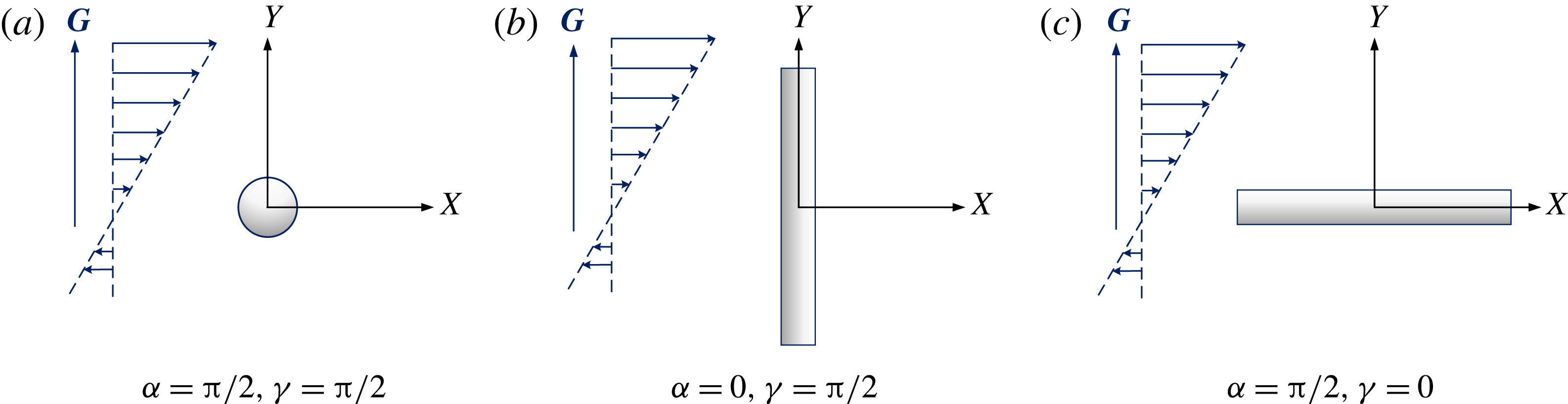
When the cylinder is in the specific orientation shown in figure 3, the transverse forces are equal to zero and the lift force for the case of figure 3(a) becomes
 $$\begin{eqnarray}\displaystyle & \displaystyle \boldsymbol{F}_{L,s}=-{\displaystyle \frac{5\unicode[STIX]{x1D70C}\unicode[STIX]{x1D706}GU_{0}RL}{2\unicode[STIX]{x03C0}}}(6\unicode[STIX]{x1D6FA}_{s,\bot ,2}^{(1,2)\ast }-\unicode[STIX]{x1D6FA}_{s,\bot ,1}^{(1,1)\ast })\boldsymbol{J}, & \displaystyle\end{eqnarray}$$
 $$\begin{eqnarray}\displaystyle & \displaystyle \boldsymbol{F}_{L,d}=-{\displaystyle \frac{5\unicode[STIX]{x1D70C}\unicode[STIX]{x1D706}GU_{0}RL}{2\unicode[STIX]{x03C0}}}(6\unicode[STIX]{x1D6FA}_{d,\bot ,2}^{(1,2)\ast }-\unicode[STIX]{x1D6FA}_{d,\bot ,1}^{(1,1)\ast })\boldsymbol{J}. & \displaystyle\end{eqnarray}$$
For the case of figure 3(b),
 $$\begin{eqnarray}\displaystyle & \displaystyle \boldsymbol{F}_{L,s}=0, & \displaystyle\end{eqnarray}$$
 $$\begin{eqnarray}\displaystyle & \displaystyle \boldsymbol{F}_{L,d}=-{\displaystyle \frac{5\unicode[STIX]{x1D70C}\unicode[STIX]{x1D706}GU_{0}RL}{2\unicode[STIX]{x03C0}}}(6\unicode[STIX]{x1D6FA}_{d,\Vert ,1}^{(1,2)\ast }-\unicode[STIX]{x1D6FA}_{d,\Vert ,1}^{(1,1)\ast })\boldsymbol{J}. & \displaystyle\end{eqnarray}$$
For the case of figure 3(c),
 $$\begin{eqnarray}\displaystyle & \displaystyle \boldsymbol{F}_{L,s}=-{\displaystyle \frac{5\unicode[STIX]{x1D70C}\unicode[STIX]{x1D706}GV_{o}RL}{2\unicode[STIX]{x03C0}}}(6\unicode[STIX]{x1D6FA}_{s,\bot ,3}^{(1,2)\ast }-\unicode[STIX]{x1D6FA}_{s,\bot ,1}^{(1,1)\ast })\boldsymbol{J}, & \displaystyle\end{eqnarray}$$
 $$\begin{eqnarray}\displaystyle & \displaystyle \boldsymbol{F}_{L,d}=-{\displaystyle \frac{5\unicode[STIX]{x1D70C}\unicode[STIX]{x1D706}GV_{o}RL}{2\unicode[STIX]{x03C0}}}(6\unicode[STIX]{x1D6FA}_{d,\bot ,3}^{(1,2)\ast }-\unicode[STIX]{x1D6FA}_{d,\bot ,1}^{(1,1)\ast })\boldsymbol{J}. & \displaystyle\end{eqnarray}$$
Three specific orientations of the cylinder with respect to the shear flow. The orientation angles are (a)
 $\unicode[STIX]{x1D6FC}=\unicode[STIX]{x03C0}/2$
and
 $\unicode[STIX]{x1D6FE}=\unicode[STIX]{x03C0}/2$
, (b)
 $\unicode[STIX]{x1D6FC}=0$
and
 $\unicode[STIX]{x1D6FE}=\unicode[STIX]{x03C0}/2$
, (c)
 $\unicode[STIX]{x1D6FC}=\unicode[STIX]{x03C0}/2$
and
 $\unicode[STIX]{x1D6FE}=0$
.

3.4 Cylinder orientation effect
The lift forces obtained in §§ 3.2 and 3.3 are instantaneous with given orientations. For a cylinder with its characteristic length much less than the mean free path of the gas, its rotation is unhindered and the cylinder orientations can be assumed to be equiprobable (i.e., a uniformly random distribution) in the absence of a strong external force field. Then, the averaged lift force on the randomly oriented cylinder may be obtained as
 $$\begin{eqnarray}\langle \boldsymbol{F}_{L}\rangle ={\displaystyle \frac{1}{4\unicode[STIX]{x03C0}}}\int _{0}^{2\unicode[STIX]{x03C0}}\int _{0}^{\unicode[STIX]{x03C0}}\boldsymbol{F}_{L}(\unicode[STIX]{x1D6FC},\unicode[STIX]{x1D6FD})\sin \unicode[STIX]{x1D6FC}\,\text{d}\unicode[STIX]{x1D6FC}\,\text{d}\unicode[STIX]{x1D6FD}.\end{eqnarray}$$
The final orientation-averaged lift force can be written as
 $$\begin{eqnarray}\langle \boldsymbol{F}_{L,s}\rangle =-{\displaystyle \frac{5\unicode[STIX]{x1D70C}\unicode[STIX]{x1D706}GV_{o}RL}{2\unicode[STIX]{x03C0}}}\left({\displaystyle \frac{2}{5}}\unicode[STIX]{x1D6FA}_{s,\bot ,1}^{(1,2)\ast }+2\unicode[STIX]{x1D6FA}_{s,\bot ,2}^{(1,2)\ast }+{\displaystyle \frac{4}{5}}\unicode[STIX]{x1D6FA}_{s,\bot ,3}^{(1,2)\ast }-{\displaystyle \frac{2}{3}}\unicode[STIX]{x1D6FA}_{s,\bot ,1}^{(1,1)\ast }\right)\boldsymbol{J}\end{eqnarray}$$
for specular scattering and
 $$\begin{eqnarray}\displaystyle \langle \boldsymbol{F}_{L,d}\rangle & = & \displaystyle -{\displaystyle \frac{5\unicode[STIX]{x1D70C}\unicode[STIX]{x1D706}GV_{o}RL}{2\unicode[STIX]{x03C0}}}\left({\displaystyle \frac{2}{5}}\unicode[STIX]{x1D6FA}_{d,\bot ,1}^{(1,2)\ast }+2\unicode[STIX]{x1D6FA}_{d,\bot ,2}^{(1,2)\ast }+{\displaystyle \frac{4}{5}}\unicode[STIX]{x1D6FA}_{d,\bot ,3}^{(1,2)\ast }\right.\nonumber\\ \displaystyle & & \displaystyle \left.-\,{\displaystyle \frac{1}{5}}\unicode[STIX]{x1D6FA}_{d,\Vert ,1}^{(1,2)\ast }+{\displaystyle \frac{2}{5}}\unicode[STIX]{x1D6FA}_{d,\Vert ,2}^{(1,2)\ast }+\unicode[STIX]{x1D6FA}_{d,\Vert ,3}^{(1,2)\ast }-{\displaystyle \frac{2}{3}}\unicode[STIX]{x1D6FA}_{d,\bot ,1}^{(1,1)\ast }-{\displaystyle \frac{1}{3}}\unicode[STIX]{x1D6FA}_{d,\Vert ,1}^{(1,1)\ast }\right)\boldsymbol{J}\end{eqnarray}$$
for diffuse scattering. For simplicity, equations (3.52) and (3.53) are written as
 $$\begin{eqnarray}\displaystyle & \displaystyle \langle \boldsymbol{F}_{L,s}\rangle =-{\displaystyle \frac{5\unicode[STIX]{x1D70C}\unicode[STIX]{x1D706}GV_{o}RL}{2\unicode[STIX]{x03C0}}}\unicode[STIX]{x1D6FA}_{s}^{\ast }\boldsymbol{J}, & \displaystyle\end{eqnarray}$$
 $$\begin{eqnarray}\displaystyle & \displaystyle \langle \boldsymbol{F}_{L,d}\rangle =-{\displaystyle \frac{5\unicode[STIX]{x1D70C}\unicode[STIX]{x1D706}GV_{o}RL}{2\unicode[STIX]{x03C0}}}\unicode[STIX]{x1D6FA}_{d}^{\ast }\boldsymbol{J}, & \displaystyle\end{eqnarray}$$
where
 $\unicode[STIX]{x1D6FA}_{s}^{\ast }$
and
 $\unicode[STIX]{x1D6FA}_{d}^{\ast }$
denote the terms in the brackets in (3.52) and (3.53), respectively. For rigid-body collisions,
 $\unicode[STIX]{x1D6FA}_{s/d}^{\ast }$
can be reduced to
 $\unicode[STIX]{x1D6FA}_{s}^{\ast }=\unicode[STIX]{x1D6FA}_{d}^{\ast }=\unicode[STIX]{x03C0}^{2}/15$
. Note that the transverse forces vanish after integrating over the uniformly random distribution of orientations.
4 Lift force on some specific examples of nanocylinders
As an example, the transport of a CNTs in argon flows is considered. In general, the gas–CNT interactions can be considered as the overall effect of the Lennard-Jones interactions between the gas molecules and all the carbon atoms of the CNT. In this sense, the gas–CNT potential function can be constructed based on the addition of the Lennard-Jones 12-6 interactions between a gas molecule and all carbon atoms of a CNT. Although there is some evidence that the potential is not linearly additive, the higher-order terms can be negligible because the dispersion interaction and electrostatic repulsion are generally localized (Liu et al. Reference Liu, Li and Wang2016a ,Reference Liu, McGivern, Manion and Wang b ). This approach has been widely used to calculate the potential of molecule–solid interactions (Girifalco, Hodak & Lee Reference Girifalco, Hodak and Lee2000; Britz & Khlobystov Reference Britz and Khlobystov2006; Watanabe et al. Reference Watanabe, Yamaguchi, Hashinokuchi, Sawabe, Maruyama, Matsumoto and Shobatake2006). In the present paper, the following potential function for the gas–CNT interactions proposed by Wong et al. (Reference Wong, Liu, Wang, Chao and Li2012) is employed,
 $$\begin{eqnarray}\displaystyle \unicode[STIX]{x1D6F7}(r)=\unicode[STIX]{x1D700}_{gas\text{-}CNT}\left[A_{1}\left({\displaystyle \frac{r-R}{\unicode[STIX]{x1D70E}_{gc}}}\right)^{n_{1}}-A_{2}\left({\displaystyle \frac{r-R}{\unicode[STIX]{x1D70E}_{gc}}}\right)^{n_{2}}\right], & & \displaystyle\end{eqnarray}$$
where
 $r$
is the distance between the gas molecule and the axis of the CNT,
 $\unicode[STIX]{x1D70E}_{gc}$
is the Lennard-Jones 12-6 collision diameter between carbon and the gas molecules, and
 $\unicode[STIX]{x1D700}_{gas-CNT}$
is the well depth for gas–CNT interactions, given by
 $$\begin{eqnarray}\unicode[STIX]{x1D700}_{gas\text{-}CNT}=A_{0}\left({\displaystyle \frac{R}{\unicode[STIX]{x1D70E}_{gc}}}\right)^{m}n_{c}\unicode[STIX]{x1D70E}_{gc}\unicode[STIX]{x1D700}_{gc}R,\end{eqnarray}$$
where
 $n_{c}=0.381$
Å
 $^{-2}$
is the number of carbon atoms per unit surface area of the CNT, and
 $\unicode[STIX]{x1D700}_{gc}$
is the well depth between carbon and the gas molecule. In (4.1) and (4.2),
 $A_{\text{1}}=0.635$
,
 $A_{\text{2}}=1.63$
,
 $n_{\text{1}}=-10.1$
,
 $n_{\text{2}}=-4.1$
,
 $A_{\text{0}}=5.81$
and
 $m=-0.86$
. The Lorentz–Berthelot mixing rule, i.e.,
 $\unicode[STIX]{x1D70E}_{gc}=(\unicode[STIX]{x1D70E}_{g}+\unicode[STIX]{x1D70E}_{c})/2$
and
 $\unicode[STIX]{x1D700}_{gc}=(\unicode[STIX]{x1D700}_{g}\unicode[STIX]{x1D700}_{c})^{1/2}$
, is used to obtain the interaction parameters, for which
 $\unicode[STIX]{x1D70E}_{c}=3.5$
Å and
 $\unicode[STIX]{x1D700}_{c}/k_{B}=33.3~\text{K}$
are employed for carbon atoms (Li & Wang Reference Li and Wang2004), and
 $\unicode[STIX]{x1D70E}_{g}=3.47$
Å and
 $\unicode[STIX]{x1D700}_{g}/k_{B}=114.0~\text{K}$
are employed for argon (Wang & Li Reference Wang and Li2011).
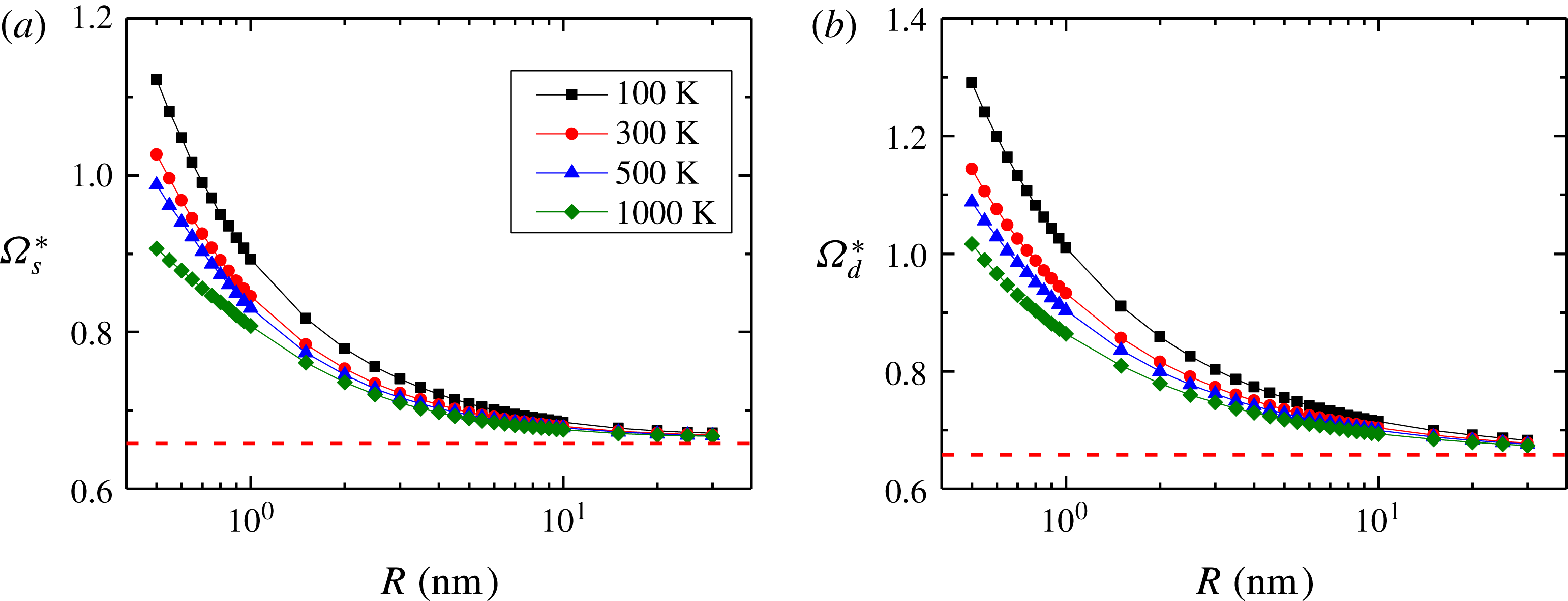
Figure 4 shows the variations of
 $\unicode[STIX]{x1D6FA}_{s/d}^{\ast }$
in (3.54) and (3.55) as a function of the CNT radius at different temperatures. In figure 4, it is clear that
 $\unicode[STIX]{x1D6FA}_{s/d}^{\ast }$
values are larger than their rigid-body limits (dashed line). The deviations from the rigid-body limits are attributed to the potential energy of the van der Waals potential between the gas molecules and the CNT. The van der Waals interactions increase the collision cross-sections, which in turn increase the reduced collision integrals and also the lift force. The non-rigid-body effect is very large for CNTs with radii of a few nanometres or below. As the radius increases, the influence of the van der Waals interaction is suppressed and the collisions tend to be rigid. Therefore, for large CNT radii,
 $\unicode[STIX]{x1D6FA}_{s/d}^{\ast }$
values, as expected, approach their rigid-body collision limits. Meanwhile, the difference in
 $\unicode[STIX]{x1D6FA}_{s/d}^{\ast }$
values between non-rigid-body collisions and rigid-body collisions is reduced with increasing temperature. As can be seen in (3.1), the scattering angle contains the ratio of the potential energy to the kinetic energy of the gas molecules. This term is integrated over the space and velocity domains to obtain the reduced collision integrals. The contribution from the potential term can be neglected for very high temperatures, because the molecular kinetic energy is much larger than the potential energy. Thus
 $\unicode[STIX]{x1D6FA}_{s/d}^{\ast }$
values are expected to converge to the rigid-body limits as
 $T\rightarrow \infty$
. Moreover, the values of
 $\unicode[STIX]{x1D6FA}_{d}^{\ast }$
are larger than those of
 $\unicode[STIX]{x1D6FA}_{s}^{\ast }$
, which is caused by a more effective momentum transport for diffuse scattering collisions than that for specular scattering collisions.
 $\unicode[STIX]{x1D6FA}_{s/d}^{\ast }$
as a function of the CNT radius at different temperature for CNT–argon interactions: (a) specular scattering, (b) diffuse scattering.

As another example of the gas–cylinder collision model, the interaction potential between gas molecules and a long-chain alkane is also employed to study the influence of the non-rigid-body effect on the lift force of a cylinder with a radius of molecular scale. The potential function of the van der Waals interactions between
 $n$
-alkane and the surrounding gas molecules takes the form (Liu et al.
Reference Liu, Li and Wang2016a
,Reference Liu, McGivern, Manion and Wang
b
)
 $$\begin{eqnarray}\unicode[STIX]{x1D6F7}(r)={\displaystyle \frac{8\unicode[STIX]{x1D700}_{gl}\unicode[STIX]{x1D70E}_{gl}}{\unicode[STIX]{x1D6FF}}}\left[0.676\left({\displaystyle \frac{r-\unicode[STIX]{x1D702}}{\unicode[STIX]{x1D70E}_{gl}}}\right)^{-11}-1.031\left({\displaystyle \frac{r-\unicode[STIX]{x1D702}}{\unicode[STIX]{x1D70E}_{gl}}}\right)^{-5}\right],\end{eqnarray}$$
where
 $r$
is the shortest distance of a gas molecule to the alkane axis,
 $\unicode[STIX]{x1D6FF}=2.514$
Å is the distance between two methylene groups,
 $\unicode[STIX]{x1D702}=0.12$
Å is a displacement factor, and
 $\unicode[STIX]{x1D700}_{gl}$
and
 $\unicode[STIX]{x1D70E}_{gl}$
are the well depth and collision diameter between a methylene group and a gas molecule. The well depth and collision diameter of the methylene group are given by
 $\unicode[STIX]{x1D700}_{\text{-CH2-}}/k_{B}=48.1$
K and
 $\unicode[STIX]{x1D70E}_{\text{-CH2-}}=4.52$
Å, respectively. Since the effective radius of a long-chain alkane approaches the molecular size, the scattering by the alkane can be regarded as a purely specular scattering. Following the method of Liu et al. (Reference Liu, Li and Wang2016a
,Reference Liu, McGivern, Manion and Wang
b
), we replace the cylinder radius
 $R$
in (3.15) and (3.16) by the collision diameter
 $\unicode[STIX]{x1D70E}_{gl}$
.
Consider the transport of an
 $n$
-alkane particle in argon. Figure 5 depicts the variations of
 $\unicode[STIX]{x1D6FA}_{s}^{\ast }$
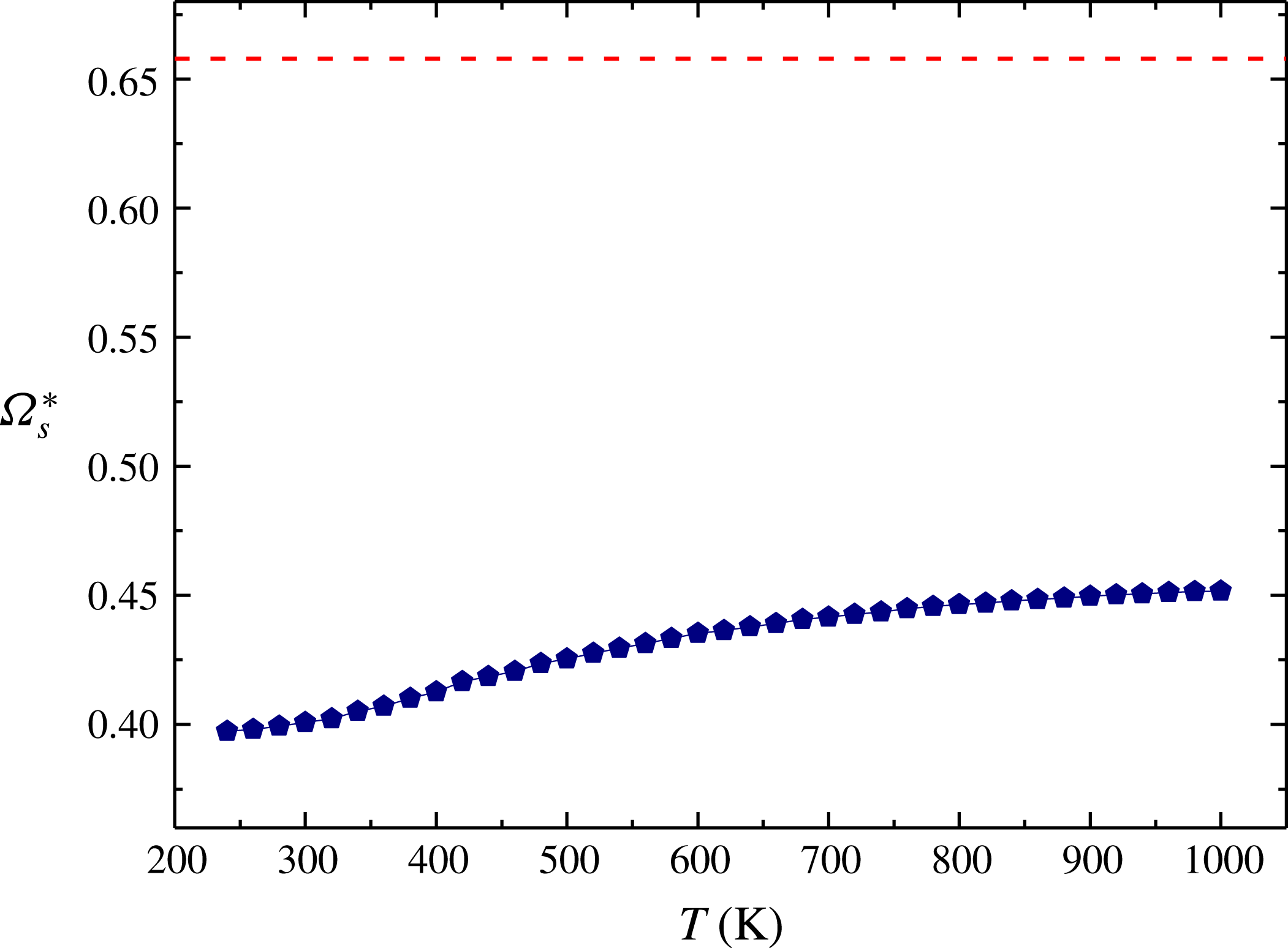
as a function of temperature. It is seen that the model of rigid-body collisions (dashed line) considerably overpredicts the lift force. The deviation from the rigid-body limit decreases as the temperature increases. In general, the van der Waals interaction has a more dramatic effect on the lift force of a long-chain
 $n$
-alkane than that of a CNT. This is probably due to the fact that an
 $n$
-alkane is much smaller than a CNT.
 $\unicode[STIX]{x1D6FA}_{s}^{\ast }$
as a function of temperature for alkane–argon interactions.

5 Conclusions
In summary, the shear lift forces on nanocylinders in shear flows at high Knudsen number have been investigated based on the gas kinetic theory. In the free molecule regime, we have obtained analytical formulae for the lift force for two limiting scattering models, namely specular and diffuse scattering, by evaluating the momentum transfer to the cylinder upon gas–cylinder collisions. The lift force formula is expressed in terms of the reduced collision integrals, which depend on the gas–cylinder intermolecular interactions. The formula based on the rigid-body collision assumption can be regarded as a special case of our current theory. The orientation effect of the cylinder is also considered in the derivation. An averaged lift force for a cylinder at random orientation is proposed by averaging the lift force over all orientations. Two examples of the gas–cylinder interactions, i.e., gas–CNT interactions and gas–alkane interactions, are employed to evaluate the lift force. It is shown that the non-rigid-body effect plays an important role for cylinders of diameter below 20 nm. The difference between the lift force under the rigid-body assumption and that under the non-rigid-body collision assumption decreases with increasing cylinder radius and/or gas temperature.
Acknowledgements
This work is supported by the National Natural Science Foundation of China (grants nos. 51776007 and 51576005), the Science and Technology Project of Beijing Education Committee (grant no. KM201610005016), and the Research Grants Council of the Hong Kong Special Administrative Region (grant no. 16228216).
Appendix A
In (3.15), (3.16) and (3.35)–(3.38),
 $\unicode[STIX]{x1D6E4}_{l}(l=1),\unicode[STIX]{x1D6EC}_{m}(m=1,2,3,4),\unicode[STIX]{x1D6F1}_{n}(n=1)$
and
 $\unicode[STIX]{x1D6F9}_{q}(q=1,2,3)$
are given as follows:
 $$\begin{eqnarray}\left.\begin{array}{@{}c@{}}\unicode[STIX]{x1D6E4}_{1}=\sin ^{3}\unicode[STIX]{x1D719}\cos ^{2}\unicode[STIX]{x1D703},\\ \unicode[STIX]{x1D6EC}_{1}=\sin ^{5}\unicode[STIX]{x1D719}\cos ^{4}\unicode[STIX]{x1D703},\\ \unicode[STIX]{x1D6EC}_{2}=\sin ^{3}\unicode[STIX]{x1D719}\cos ^{2}\unicode[STIX]{x1D719}\cos ^{2}\unicode[STIX]{x1D703},\\ \unicode[STIX]{x1D6EC}_{3}=\sin ^{5}\unicode[STIX]{x1D719}\sin ^{2}\unicode[STIX]{x1D703}\cos ^{2}\unicode[STIX]{x1D703},\\ \unicode[STIX]{x1D6EC}_{4}=\sin ^{3}\unicode[STIX]{x1D719}\cos ^{2}\unicode[STIX]{x1D719}\sin ^{2}\unicode[STIX]{x1D703},\\ \unicode[STIX]{x1D6F1}_{1}=\sin ^{3}\unicode[STIX]{x1D719}\sin ^{2}\unicode[STIX]{x1D703},\\ \unicode[STIX]{x1D6F9}_{1}=\sin ^{5}\unicode[STIX]{x1D719}\sin ^{2}\unicode[STIX]{x1D703}\cos ^{2}\unicode[STIX]{x1D703},\\ \unicode[STIX]{x1D6F9}_{2}=\sin ^{5}\unicode[STIX]{x1D719}\sin ^{4}\unicode[STIX]{x1D703},\\ \unicode[STIX]{x1D6F9}_{3}=\sin ^{3}\unicode[STIX]{x1D719}\cos ^{2}\unicode[STIX]{x1D719}\sin ^{2}\unicode[STIX]{x1D703}.\end{array}\right\}\end{eqnarray}$$
If the gas–cylinder interactions are treated as rigid-body collisions, the values of the reduced collision integrals for specular scattering,
 $\unicode[STIX]{x1D6FA}_{s,\bot ,l}^{(1,1)\ast }\,(l=1)$
,
 $\unicode[STIX]{x1D6FA}_{s,\bot ,m}^{(1,2)\ast }\,(m=1,2,3,4)$
can be theoretically obtained as
 $$\begin{eqnarray}\left.\begin{array}{@{}c@{}}\unicode[STIX]{x1D6FA}_{s,\bot ,1}^{(1,1)\ast }={\displaystyle \frac{\unicode[STIX]{x03C0}^{2}}{2}},\\ \unicode[STIX]{x1D6FA}_{s,\bot ,1}^{(1,2)\ast }={\displaystyle \frac{5\unicode[STIX]{x03C0}^{2}}{16}},\\ \unicode[STIX]{x1D6FA}_{s,\bot ,2}^{(1,2)\ast }={\displaystyle \frac{5\unicode[STIX]{x03C0}^{2}}{48}},\\ \unicode[STIX]{x1D6FA}_{s,\bot ,3}^{(1,2)\ast }={\displaystyle \frac{\unicode[STIX]{x03C0}^{2}}{12}},\\ \unicode[STIX]{x1D6FA}_{s,\bot ,4}^{(1,2)\ast }={\displaystyle \frac{\unicode[STIX]{x03C0}^{2}}{12}},\end{array}\right\}\end{eqnarray}$$
while the values of the reduced collision integrals for diffuse scattering,
 $\unicode[STIX]{x1D6FA}_{d,\bot ,l}^{(1,1)\ast }\,(l=1)$
,
 $\unicode[STIX]{x1D6FA}_{d,\bot ,m}^{(1,2)\ast }\,(m=1,2,3,4)$
,
 $\unicode[STIX]{x1D6FA}_{d,\Vert ,n}^{(1,1)\ast }\,(n=1)$
, and
 $\unicode[STIX]{x1D6FA}_{d,\Vert ,q}^{(1,1)\ast }\,(q=1,2,3,4)$
are
 $$\begin{eqnarray}\left.\begin{array}{@{}c@{}}\unicode[STIX]{x1D6FA}_{d,\bot ,1}^{(1,1)\ast }={\displaystyle \frac{6\unicode[STIX]{x03C0}^{2}+\unicode[STIX]{x03C0}^{3}}{16}},\\ \unicode[STIX]{x1D6FA}_{d,\bot ,1}^{(1,2)\ast }={\displaystyle \frac{2\unicode[STIX]{x03C0}^{3}+15\unicode[STIX]{x03C0}^{2}}{64}},\\ \unicode[STIX]{x1D6FA}_{d,\bot ,2}^{(1,2)\ast }={\displaystyle \frac{2\unicode[STIX]{x03C0}^{3}+15\unicode[STIX]{x03C0}^{2}}{192}},\\ \unicode[STIX]{x1D6FA}_{d,\bot ,3}^{(1,2)\ast }={\displaystyle \frac{\unicode[STIX]{x03C0}^{3}+6\unicode[STIX]{x03C0}^{2}}{96}},\\ \unicode[STIX]{x1D6FA}_{d,\bot ,4}^{(1,2)\ast }={\displaystyle \frac{\unicode[STIX]{x03C0}^{3}+6\unicode[STIX]{x03C0}^{2}}{96}},\\ \unicode[STIX]{x1D6FA}_{d,\Vert ,1}^{(1,1)\ast }={\displaystyle \frac{\unicode[STIX]{x03C0}^{2}}{4}},\\ \unicode[STIX]{x1D6FA}_{d,\Vert ,1}^{(1,2)\ast }={\displaystyle \frac{\unicode[STIX]{x03C0}^{2}}{16}},\\ \unicode[STIX]{x1D6FA}_{d,\Vert ,2}^{(1,2)\ast }={\displaystyle \frac{\unicode[STIX]{x03C0}^{2}}{8}},\\ \unicode[STIX]{x1D6FA}_{d,\Vert ,3}^{(1,2)\ast }={\displaystyle \frac{\unicode[STIX]{x03C0}^{2}}{16}}.\end{array}\right\}\end{eqnarray}$$