


1. Introduction: Evolution in bond markets
Sovereign bond markets are huge. Government debt surpassed $100 trillion in 2024—this is around 90% of global GDP (UNCTAD, 2025). Each day, about US $900 billion of US Treasuries change hands (FINRA, 2025). This scale is new: governments issued $25 trillion in 2024 alone, almost triple the level in 2007 (OECD, 2025). Within advanced economies, issuance is particularly high: the OECD predicts that bond issuance by its members was $17 trillion in 2025.
As quantities have changed, so have prices and yields. Over the past 3 years, bond market prices have been notably unstable at key periods in the policymaking cycle. A familiar pattern has emerged. Policies with fiscal implications are announced. Bond yields rise quickly (prices fall), forcing leaders and finance ministers to make statements to calm markets. These often amount to the adjustment, or cancellation, of the previous policy announcement. The bond market constraint on policy seems to bind more tightly.
This has been seen across the G7. In Germany, the least indebted of the G7 economies, announcements of a new fiscal package in March led to the biggest bond-market jump since the fall of the Berlin Wall (De Vijlder, Reference De Vijlder2025). In the United States, President Trump’s initial ‘Liberation Day’ tariff plans led to bond selloffs and changes in policy (Financial Times, 2025). In France, rising bond yields have played a significant role in the collapse of the Bayrou government in September 2025. In Japan, weak demand in 20- and 40-year bond auctions led to yields spiking in May 2025 (JP Morgan, Reference Morgan2025). In the United Kingdom, the finance minister’s Growth Plan 2022 led to bond market volatility that ultimately required central bank intervention.
Understanding the G7 fiscal constraint is important in its own right, and also as a guide to the path other countries may be on. Of the 20 most-populous countries in the world, all are projected by the IMF (2025) to run a deficit in 2025, ranging from 2% in Russia and Ethiopia to 12% of GDP in Egypt. For example, Nigeria’s leader, Bola Tinubu, has a policy package to equalise infrastructure quality—mainly road and rail—across the nation. This will require $21 billion of borrowing (Alli, Reference Alli2025). Bond markets globally will play a vital part in the financing of such plans.
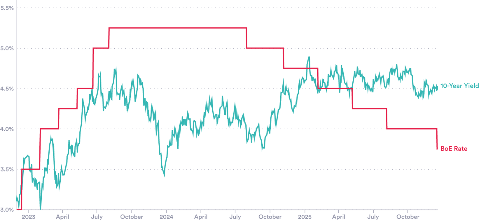
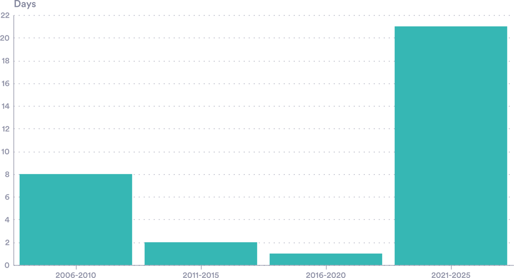
These recent size shifts in bond markets have been accompanied by two puzzling features. First, the relationship between changes in central bank rates and bond yields seems to have weakened (Figure 1). Second, yields have become markedly more volatile, showing instability not seen in many countries since the financial crisis. Documenting and explaining these two observations is the key aim of this paper (Figure 2).
Puzzle 1— Policy and market rates. UK 10-Year bond yield and interest rate.
Source: LSEG Workspace (yields), Bank of England.
Note: Market Yield on UK Treasury Securities at 10-Year Constant Maturity. An equivalent US figure is included in the Supplementary Material.Footnote 1

Figure 1. Long description
The Y-axis represents percentage rates ranging from 3.0 percent to 5.5 percent in 0.5 percent increments. The X-axis spans from early 2023 to late 2025, marked by quarterly intervals.
* The B o E Rate is depicted as a red stepped line. It begins at 3.0 percent in early 2023, rises in steps to a peak of 5.25 percent by late 2023, maintains this plateau through mid-2024, and then descends in steps to 4.0 percent by late 2025.
* The 10-Year Yield is shown as a jagged teal line. It starts near 3.2 percent, fluctuates with a general upward trend to peak near 4.8 percent in late 2023, drops sharply to 3.5 percent in early 2024, and then recovers to fluctuate between 4.3 percent and 4.8 percent throughout 2025.
By the end of the period, the teal yield line remains higher than the red B o E rate line.
Puzzle 2—Increased volatility. Days with a UK 10-Y gilt intraday range of over 0.25 bps.
Source: Authors’ calculations via data from LSEG (2025).
Note: The number of individual days with a high–low range of over 25 bps, by 5-year (year start–year end) period.

Central banks’ ability to control long rates ebbs and flows. In 2005, for example, Alan Greenspan famously set out the ‘conundrum’ of why 10-year US Treasury yields had remained essentially unchanged despite the Federal Reserve’s policy rate increasing by 150 basis points (see, for example, Thornton, Reference Thornton2018). In the year to August 2024, 10-year yields in the United Kingdom and the United States moved a lot, despite no policy rate change. Since then, the policy rate has been cut sharply, falling from 5.25% to 3.75% in the United Kingdom—long yields did not follow, and even rose somewhat. It is akin to Greenspan’s Conundrum, but in reverse.
Volatility has increased too. Examining the daily changes in bond yields suggests that the past 5 years (calendar years 2021–2025) are more volatile than the preceding period (2005–2020) in the United Kingdom, Germany and France. Given that the Footnote earlier period includes the GFC, euro-crisis and the pandemic, this is surprising. Taking the United Kingdom as an example and using a daily change of 25 basis points as a simple benchmark for a large move reveal 21 daily swings of this level in the five years to 2025 (Figure 2). We see a similar pattern in Germany and France, but not in the United States and Canada, where the GFC period is more volatile.
Both the level and volatility of sovereign bond yields are somewhat puzzling. This adds to policy uncertainty: bond markets are a clear constraint on policy, but one that is shifting in ways that are not clear. What is driving bond yields—both their elevated level, and their tendency to suddenly spike—and what does this mean for fiscal policymakers? This paper aims to provide early answers to these questions.
The analysis proceeds as follows. Section 2 provides an up-to-date analysis of the sovereign bond market, examining changes in the issuance, holdings and demand for government debt. Section 3 reviews determinants of yields and commonly used models and examines the evolution of both yields and volatility. We then posit potential influences, including hedge fund activity, foreign holdings of debt and fiscal institution activity. Section 4 concludes.
2. Market developments: Issuers, purchasers and trends
2.1. Supply: Exceptional issuance
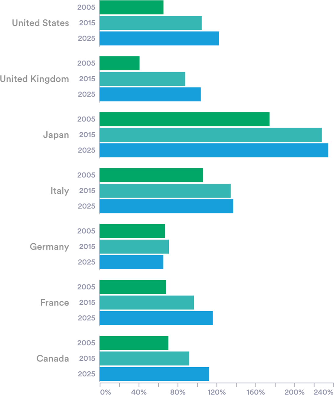
One reason for concern about elevated bond yields is simply the scale of G7 economies’ reliance on bond markets over the past 5 years. The total debt outstanding in G7 countries was estimated at around US$60 trillion in 2024, or 125% of the countries’ joint GDP. The United States, the largest debtor in nominal terms, accounted for around $35 trillion, while Japan carried the heaviest burden relative to GDP (around 235%). Germany is now the only G7 member with a debt-to-GDP ratio below 100% (Figure 3).
G7 countries’ rising debt burden. Gross debt as a percentage of GDP.
Source: IMF Fiscal Monitor (2025).
Note: Figures for 2025 are projections.

Figure 3. Long description
The chart features seven country groups. The x-axis ranges from 0 percent to 240 percent in increments of 40. Each country has three bars: green for 2005, teal for 2015, and blue for 2025.
* United States: Debt increases from approximately 65 percent in 2005 to 105 percent in 2015 and 130 percent in 2025.
* United Kingdom: Debt increases from 40 percent in 2005 to 90 percent in 2015 and 105 percent in 2025.
* Japan: The highest debt levels, starting at 175 percent in 2005, rising to 235 percent in 2015, and reaching nearly 250 percent in 2025.
* Italy: Debt increases from 105 percent in 2005 to 135 percent in 2015 and 140 percent in 2025.
* Germany: Debt remains relatively stable, starting at 70 percent in 2005, peaking at 75 percent in 2015, and projected to decrease slightly to 65 percent in 2025.
* France: Debt increases from 70 percent in 2005 to 100 percent in 2015 and 115 percent in 2025.
* Canada: Debt increases from 70 percent in 2005 to 95 percent in 2015 and 115 percent in 2025.
In practical terms, governments raise funds by selling bonds at auctions. The strategies used differ across the G7. The United States holds more than 400 auctions a year, while France conducts less than one per week. Auctions conducted in 2025 have been met with lower market demand and rising yields, especially for long-term bonds. For example, auctions of 30-year Japanese Government Bonds (JGBs) during the first half of 2025 received lower than expected bid-to-cover ratios (CEIC, 2025). Recent auctions of US long-term bonds have similarly seen falling demand (Chavez-Dreyfuss, Reference Chavez-Dreyfuss2025).
2.2. Bond holdings: Shifting demand?
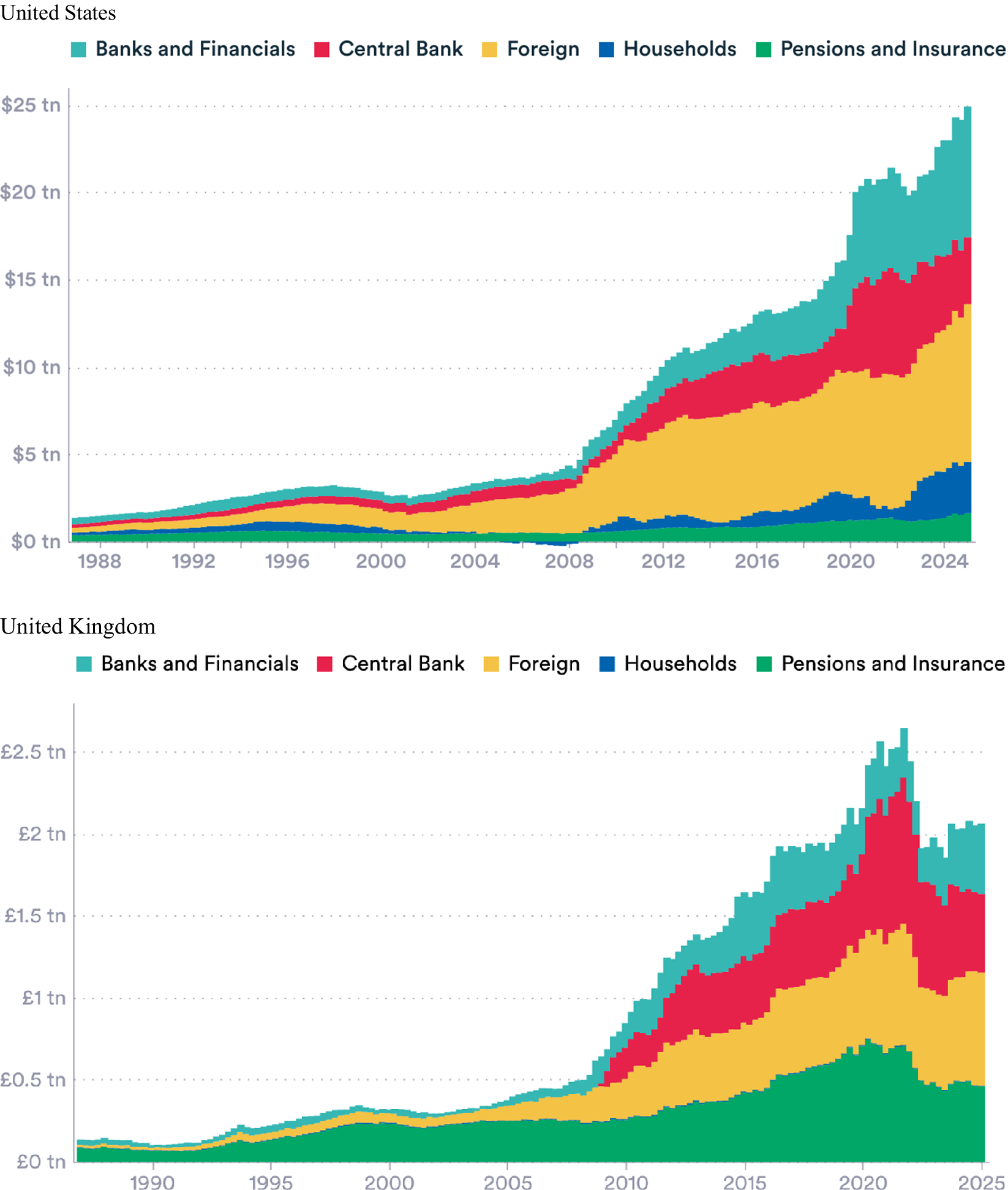
While supply has been expanding year on year, it has not been met by steady, reliable demand. The holdings by various sectors have changed (Figure 4, and Figures 1, 2 and 3 in the Supplementary Material). Several developments have shifted purchases of sovereign bonds: this includes changes in foreign exchange reserve strategies, central bank policy decisions, hedge fund strategies, stablecoin projects and pension fund regulation. This section describes each of these trends.
Debt composition, the United States and the United Kingdom. Nominal debt, by institutional holder.
Source: US Federal Reserve—Financial Accounts of the United States (Z1)—L210 (via FRED, 2025), ONS—UK Economic Accounts: institutional sector—general government—5.2.12B.
Note: Negative public debt holdings occur when a sector has a net short position from repurchase agreements, ‘Households’ includes NPISH.

Figure 4. Long description
The image consists of two panels.
Top Panel: United States.
The x-axis represents years from 1988 to 2025. The y-axis represents nominal debt in U S dollars, ranging from $0 tn to $25 tn. The data is presented as a stacked area chart with five categories. From bottom to top, the layers are:
* Pensions and Insurance (green): Maintains a thin, relatively stable base near the zero line.
* Households (dark blue): A thin layer that shows slight expansion after 2010.
* Foreign (yellow): A significant and widening band that grows steadily from the early 2000s.
* Central Bank (red): A layer that remains negligible until 2008, then expands rapidly in distinct steps corresponding to 2009, 2013, and 2020.
* Banks and Financials (teal): The top layer, which shows the most significant growth after 2018, reaching the $25 tn peak by 2025.
Bottom Panel: United Kingdom.
The x-axis represents years from 1990 to 2025. The y-axis represents nominal debt in British pounds, ranging from £0 tn to £2.5 tn. The stack order differs slightly in visual prominence:
* Pensions and Insurance (green): Forms the largest base layer, showing a significant upward trend starting around 2008.
* Households (dark blue): A very thin, almost negligible layer between green and yellow.
* Foreign (yellow): A substantial layer that grows consistently from 2005 onwards.
* Central Bank (red): Shows a massive expansion starting in 2009, peaking around 2021 before slightly contracting.
* Banks and Financials (teal): The uppermost layer, which fluctuates significantly, peaking around 2021 and then declining toward 2025.
Both charts show a sharp exponential increase in total debt starting around the 2008 financial crisis, with a second major acceleration occurring around 2020.
2.2.1. Foreign exchange reserves
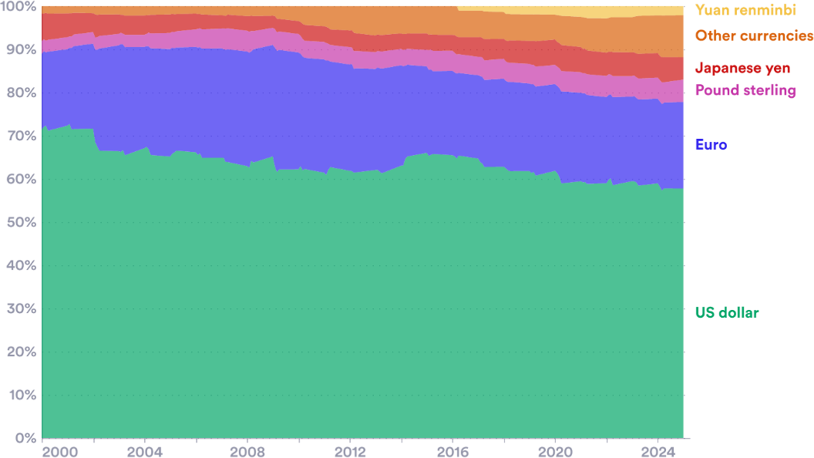
Most states hold reserve assets denominated in foreign currencies. These reserves are tracked by the IMF in its COFER database and they stood at around $12.8 trillion in 2024. These holdings are often channelled into sovereign debt. The US dollar is still by far the most important currency, but its share has fallen from around 70% in 2000 to just under 60% today (Figure 5). The decline stems both from reserve accumulation by countries that tend to hold few dollars, including China and India, and the diversification by a few large reserve holders, including Russia and Switzerland, perhaps driven by geopolitics (Goldberg and Hannaoui, Reference Goldberg and Hannaoui2024).
Global composition of currency denominated reserves by currency. Reserve currencies as a percentage of global foreign exchange reserves.
Source: Authors’ elaboration of IMF COFER dataset.
Note: Figures for 2025 are projections.

Figure 5. Long description
The x axis represents time from the year 2000 to 2025. The y axis represents the percentage of global foreign exchange reserves from 0 percent to 100 percent. The data is presented as a stacked area chart with six categories.
* U S dollar (green): Occupies the bottom layer, starting at approximately 71 percent in 2000 and showing a gradual downward trend to just below 60 percent by 2025.
* Euro (purple): The second layer, maintaining a relatively stable share between 20 percent and 25 percent throughout the period.
* Pound sterling (pink): A thin band above the Euro, remaining consistent at around 5 percent.
* Japanese yen (red): Positioned above the Pound sterling, also holding a steady share of approximately 5 percent.
* Other currencies (orange): This layer shows a visible expansion, growing from a negligible sliver in 2000 to nearly 10 percent by 2025.
* Yuan renminbi (yellow): The top-most layer, which appears around 2016 and grows to a small but distinct percentage by 2025.
The overall trend shows a decline in the U S dollar's dominance as other currencies and the Yuan renminbi increase their shares.
Most G7-currency-denominated reserves are held outside the G7. (The G7 economies’ reserves are relatively low, at 1.9 trillionFootnote 2 or 16% of the global total.) While the IMF does not disclose countries’ individual positions in the COFER database, other sources show the reliance on G7 currencies. China holds US$3.3 trillion in foreign exchange assets (SAFE 2025). Almost all are G7 currencies: roughly 60% in US dollars, 20% in euros, 7.5% in pounds and 5% in yen (Ferranti, Reference Ferranti2023). Russia has also historically retained most of its foreign exchange assets in G7 currencies, favouring euros over dollars. (Bank of Russia, 2022).Footnote 3 Russia’s reserve composition is believed to have shifted since the invasion of Ukraine (Stognei, Reference Stognei2025).
These are examples of how decisions taken outside the G7 could also be having an impact on demand, pricing and yields. An important potential development is proposals for a new ‘BRICS’ reserve currency. It would be a way to settle international trade between BRICS partners without relying on reserve currencies like the dollar or euro. At present, these countries are focused on increasing the share of trade among themselves in local currencies—this trend may reduce demand for G7-denominated assets (Reuters, 2025).
2.2.2. Central Banks—Quantitative tightening
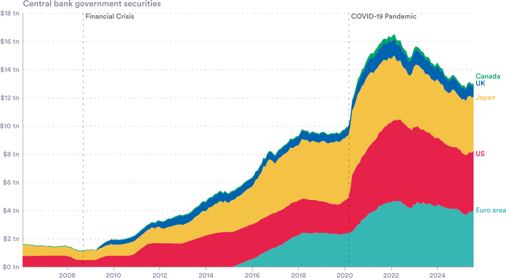
After the 2008 GFC and the 2020 pandemic, central banks bought bonds at a huge scale (Figure 6). In total, G7 Central Bank holdings of government securities increased by $15 trillion between the GFC and their 2022 peak. The strategy—quantitative easing (QE)—aimed to boost demand leading to higher bond prices, lower yields and an economy-wide stimulus. Studies across the United Kingdom, the United States and the euro area suggest QE purchases worth 10% of GDP result in median reductions in yields of around 45 to 55 basis points for 10-year government bonds (Gagnon, Reference Gagnon2016).
Central bank holdings of government securities. Inclusive of bonds and short-term debt in G7 countries.
Note: The UK and ECB report holdings of government securities for the purposes of quantitative easing in segregated accounts (APF and APP/PEP, respectively). Figures for Japan, the United States and Canada are total holdings. Values are converted into USD using contemporaneous exchange rates prevailing on each observation date. Sources: Bank of England via ONS, Bank of Japan via LSEG Workspace, Bank of Canada, ECB, US Federal Reserve via FRED.

Figure 6. Long description
The x-axis represents time from 2008 to 2024. The y-axis represents value in trillions of U S dollars, ranging from $0 t n to $18 t n. Two vertical dashed lines mark the Financial Crisis in late 2008 and the C O V I D-19 Pandemic in early 2020.
The data is presented as a stacked area chart with five layers, listed from bottom to top:
* Euro area (teal): Starts near zero in 2015, rising to approximately $4 t n by 2022 before a slight decline.
* U S (red): Maintains a steady base, expanding significantly after 2008 and 2020 to reach a peak around $6 t n of the total stack.
* Japan (yellow): Shows a consistent, thick band that grows steadily from 2013 onwards.
* U K (dark blue): A thinner band representing holdings that increased notably after 2009 and 2020.
* Canada (green): The thinnest band at the top of the stack.
Trend analysis: Total holdings remained below $2 t n until 2009. They rose steadily to $10 t n by 2020. Following the C O V I D-19 Pandemic line, there is a sharp vertical spike reaching a peak of over $16 t n in 2022, followed by a gradual decline to approximately $13 t n by 2024.
In recent years, central banks have started to sell bonds, a policy known as quantitative tightening (QT). This has meant allowing maturing bonds to roll off their balance sheets and, in some cases, active sales.Footnote 4 Since the March 2022 peak, G7 central banks have shed $3.5 trillion of government bonds, 21% of their total holdings.
Research suggests QT can have sizeable price and yield effects. In some cases, surprise QT announcements have been larger in magnitude than the inverse effects of QE (D’Amico and Seida, Reference D’Amico and Seida2024; Lloyd and Ostry, Reference Lloyd and Ostry2024). Bank of England research estimates that a ‘full-flow’ QT—allowing all maturing gilts to expire without reinvestment—would increase 10-year yields by around 20 basis points under low-stress market conditions (Joyce and Lengyel, Reference Joyce and Lengyel2024).
2.2.3. Hedge funds
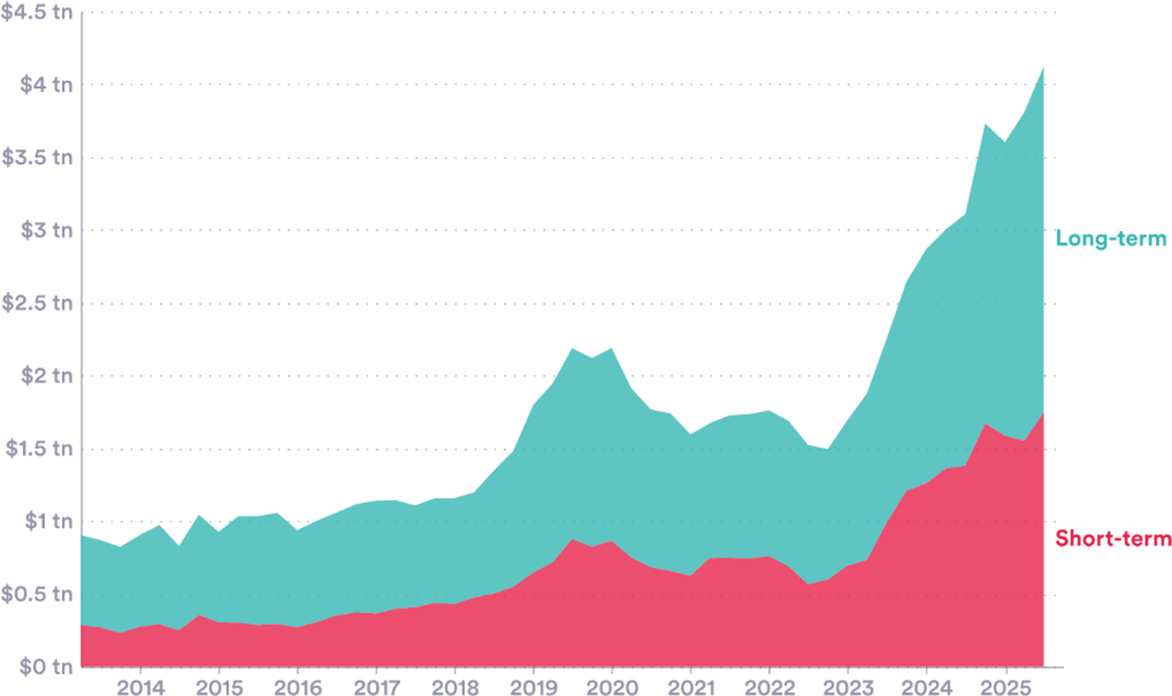
The role hedge funds play is increasing in importance. While transparent data on hedge fund holdings are hard to access, the available statistics point to rapid increases in sovereign bond holdings in recent years. In the United States, official data show hedge fund holdings of government bonds at record highs (Figure 7).Footnote 5
Hedge funds holdings of US Government bonds. US Treasury exposures to qualifying hedge funds.
Source: Hedge Fund Monitor, Office of Financial Research (2025).

Figure 7. Long description
The X axis represents time in years from 2014 to 2025. The Y axis represents value in U S dollars, ranging from $0 tn to $4.5 tn in increments of $0.5 tn. The data is presented as a stacked area chart with two categories.
* Short-term: Represented by the bottom pink layer. It remains relatively stable between $0.25 tn and $0.5 tn from 2014 until 2018. It shows a moderate peak near $0.8 tn in 2020, followed by a slight decline, and then a sharp exponential increase starting in 2023, reaching approximately $1.7 tn by 2025.
* Long-term: Represented by the top teal layer stacked above the short-term data. This category follows a similar trend but with higher volatility. It shows a significant peak in 2020 at a combined total of roughly $2.2 tn. After a dip in 2021 and 2022, it experiences a massive surge beginning in 2023.
The total combined exposure reaches its highest point at the end of the timeline in 2025, surpassing $4 tn.
Hedge funds play a complex role in bond markets. They provide liquidity and improve market functioning: the high volume of bonds bought and sold makes it easier for others to execute trades (in 2023, hedge funds accounted for 56% of trading volume in the secondary market in Europe; Ferrara et al., Reference Ferrara, Linzert, Nguyen, Rahmouni-Rousseau, Skrzypińska and Vaz Cruz2024). Arbitrage activity can play an important role in accurate price discovery.
Recent events have also shown that hedge funds can add volatility, and their growing involvement may explain some of the increased volatility in bond markets seen in recent years. One case is the popular strategy known as the cash-futures ‘basis trade’ (Glicoes et al., Reference Glicoes, Iorio, Monin and Petrasek2024). Hedge funds aim to profit from small differences in the price of government bonds and of the futures contracts related to them.Footnote 6
The risk comes from leverage. In this basis trade, price differentials are small, so substantial leverage is used to magnify positions and potential returns. (Traders have used median leverage ratios as high as 15 times the capital investment, Barth and Kahn, Reference Barth and Kahn2025). This, in turn, means that unwinding a position can mean selling a large quantity of bonds, potentially impacting the price.
In the United States, the unwinding of basis trades is thought to have contributed to market stress in 2020. In the face of economic shutdown, hedge funds unwound their positions, selling US Treasuries, putting downward pressure on prices. At this time, the average fund following this strategy reduced its treasury exposure by close to 20% (Kruttli et al, Reference Kruttli2021). In the US treasury market during the period 9–18 March, the 10-year yield surged by 64 basis points (Vissing-Jørgensen, Reference Vissing-Jørgensen2021). Since this period, hedge fund exposures have increased significantly.
Similar concerns are seen in other G7 nations. In Japan, trading activity in the JGB market doubled between 2022 and 2024.Footnote 7 In the United Kingdom, hedge funds’ share of government debt trading volumes has increased in recent years (Mackenzie and Rovnick, Reference Mackenzie and Rovnick2025). The share of the Government of Canada bond auctions allocated to hedge funds has increased from 0% to 40% over the last 15 years (Epp and Gao, Reference Epp and Gao2025). Across the G7, hedge funds have emerged as both providers of liquidity and as potential amplifiers of volatility.
2.2.4. Stablecoins
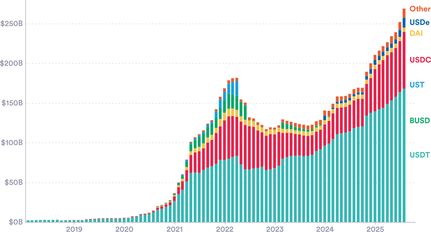
A stablecoin is a type of cryptocurrency that is linked to a traditional asset—such as a fiat currency—aiming to provide a more stable value than pure (unlinked) cryptocurrencies like Bitcoin or Ethereum. Usage has risen sharply over the past 5 years. Issuer companies link or ‘back’ the coins by purchasing reserves of the chosen asset, usually currencies or short-term bonds. For example, Tether (USDT), the most widely used stablecoin, is tied to the US dollar. Theoretically, stablecoin issuers should have reserves matching one-to-one with the number of coins in circulation. This creates a potential link between stablecoin usage and demand for G7 countries’ bonds (Figure 8).
Stablecoins by market capitalization. Leading stablecoins, September 2025.
Source: CoinMarketCap (2025).

Figure 8. Long description
The X-axis represents time from 2019 to late 2025. The Y-axis represents market capitalization in U S dollars, ranging from 0 B to 250 B in 50 B increments. The data shows a flat baseline until 2021, followed by a sharp rise to a peak of approximately 180 B in early 2022. A decline and plateau follow through 2023, before a significant growth phase starting in 2024 that exceeds 250 B by late 2025.
From bottom to top, the stacked categories are:
* U S D T (teal): The largest and most consistent base layer, growing steadily to over 150 B.
* B U S D (green): Significant presence in 2021 and 2022, but tapers off almost completely by 2024.
* U S T (light blue): A visible segment that disappears abruptly in mid-2022.
* U S D C (pink): The second-largest segment, showing substantial growth from 2021 onwards.
* D A I (yellow): A thin, consistent layer above U S D C.
* U S D e (dark blue): A new segment appearing in 2024 and expanding through 2025.
* Other (orange): The top-most thin layer representing smaller stablecoins.
Recent changes to the US regulatory system support the expansion. In July 2025, the GENIUS Act established a new regulatory system. It requires coins to be 100% reserve backed with liquid assets and for the reserve composition to be published. Around 99% of the global stablecoin market is made up of US dollar-denominated coins (JP Morgan, Reference Morgan2025). As of 2025, Q2 Tether held $127 billion in US treasuries: this is more than Germany and comparable to Saudi Arabia’s holdings.Footnote 8
The scale of stablecoins makes them another potential influence on G7 bond pricing. The first-order effect seems likely to be positive: higher usage along with the 1:1 reserve requirement may offer a new demand for US bonds. A second-order effect may be on the shape of the yield curve: stablecoin promoters may have a particular demand for short-term sovereign debt, for liquidity purposes. This could alter (steepen, in this case) the yield curve by changing the spread between bonds of different maturities (Ahmed and Aldasoro, Reference Ahmed and Aldasoro2025).
There are reasons for caution, however. A stablecoin company has similarities with a bank (or money market mutual fund) and could be prone to depositor flight. If coin holders lost confidence that the coin issuer held sufficient reserve assets, a ‘run’ on the coin could start—with many coin holders simultaneously requesting conversion back to traditional currencies. The issuer would need to sell large quantities of government bonds putting downward pressure on prices and increasing yields. Early experience with stablecoins suggests this kind of scenario is worthy of serious consideration.Footnote 9
2.2.5. Pension funds—Regulation
Pension funds and life insurers collect premiums and make investments to fund future payments to retirees and insured policyholders. They are large-scale buyers of long-dated high-quality sovereign bonds, because these bonds provide predictable payments far into the future. The three principal ways these institutions are regulated all have an impact on bond demand:
-
• Prudential or solvency rules. Ensure the fund remains solvent by aligning assets with liabilities and requiring them to hold capital against risks. Stricter regimes push funds to buy more low-risk, long-dated government bonds.
-
• Conduct and governance rules. Require sound risk management (e.g. liquidity buffers, collateral for derivatives and stress tests), which favours holding safe, liquid sovereign bonds.
-
• Product rules. Defined benefit (DB) schemes, which promise a fixed pension, typically generate heavy demand for ultra-long bonds to hedge promises. Defined contribution (DC) schemes, where savers bear investment risk, are less bond-intensive.
Changes in pension fund regulation can thus impact bond markets. This relationship depends on the size and structure of each country’s pension sector. Pension fund regulation has the largest impact in countries with significant pension-related holdings, such as Japan, where over 20% of bonds are owned by life insurers or pension funds (Glass, Reference Glass2025).
A general G7 trend in recent years has been towards tighter solvency rules and a shift from DB to DC. Many are moving towards ‘economic value’ solvency regimes that increase interest rate sensitivity and encourage long-dated bond holdings (this includes Japan’s J-ICS reform, which came into force in April 2025, and the EU’s refinement of Solvency II). The United Kingdom is also joined by the Netherlands in a shift towards DC schemes (The United States uses DC-equivalent 401(k) plans, meaning relatively less structural bond demand from pension funds).
Japan provides a recent example of regulation-driven bond volatility. Ahead of the introduction of the new solvency regime (J-ICS) this year, life insurers had spent years increasing their holdings of long-term government bonds to match their liabilities under the stricter framework. Once this was complete, demand for sovereign bonds fell sharply, resulting in a sudden spike in long-end yields. Yields on 30-year bonds rose to around 3.2%, and those on 40-year bonds to over 3.6%, their highest levels in decades. In response, the Ministry of Finance cut the supply (i.e. issuance) of long bonds to stabilise borrowing costs. It is an example of how governments must closely monitor large, structural demand for their bonds, aiming to align supply and demand.
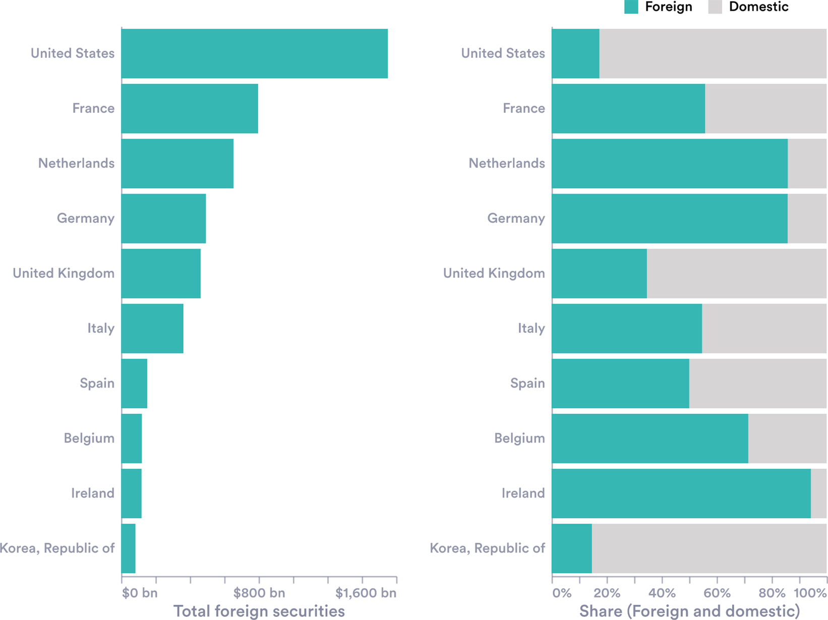
The way pension and insurance funds invest varies considerably across countries. These are shown in Figure 9 (for both sovereign and corporate bond holdings). Whereas US funds are mostly invested in domestic bonds, funds in the Netherlands, Germany and Ireland are mostly invested abroad. Where these holdings are large, they therefore have the potential to influence foreign markets. Dutch pension fund assets are huge (147% of GDP), and 27% of their long-term holdings were held in sovereign bonds in 2024, mostly from EU nations, worth €429 billion (DNB, 2025). The implication is that regulatory decisions made in The Hague could have knock-on effects for the fiscal conditions in London or Washington DC.
Pension and insurance firm holdings of debt securities. Holdings of domestic and international debt securities (left), both private and public; and the foreign–domestic share (right).
Source: Author’s calculations using BIS (2025) data.

Figure 9. Long description
The left panel is a horizontal bar chart titled Total foreign securities with an x-axis ranging from $0 b n to $1,600 b n. The bars represent the total value of foreign debt securities held by firms in each country. From top to bottom, the values are: United States at approximately $1,800 b n, France at $800 b n, Netherlands at $650 b n, Germany at $550 b n, United Kingdom at $500 b n, Italy at $400 b n, Spain at $200 b n, Belgium at $150 b n, Ireland at $150 b n, and Korea, Republic of at $100 b n.
The right panel is a stacked horizontal bar chart titled Share (Foreign and domestic) with an x-axis from 0% to 100%. Teal represents Foreign and light gray represents Domestic. The bars show the following foreign shares: United States at 15%, France at 55%, Netherlands at 85%, Germany at 85%, United Kingdom at 35%, Italy at 55%, Spain at 50%, Belgium at 70%, Ireland at nearly 100%, and Korea, Republic of at 15%.
2.2.6. Demographics
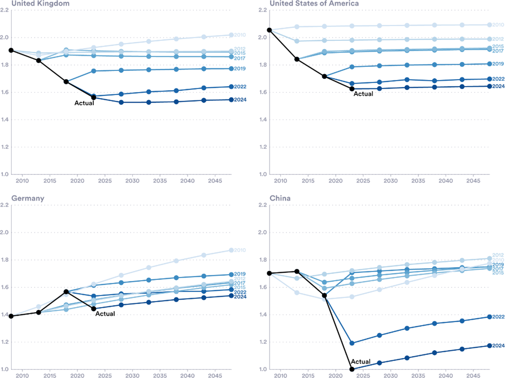
Another trend that may be driving changes in yields is investor re-evaluations of the demographic shifts that countries face. It is well known that advanced economy populations are ageing rapidly. Japan, for example, has the highest old-age dependency ratio in the world, with more than 50 people aged 65 or over for every 100 working-age adults (see Figure 10). This trend is likely to have many economic consequences. Older populations are associated with lower productivity and investment (Bodnár and Nerlich Reference Bodnár and Nerlich2022). A smaller labour force also reduces a nation’s tax base, making running primary surpluses harder and debt accumulation more likely.
Actual and projected total fertility rate. UN population projections by year of release and actual population estimates.
Source: United Nations, World Population Prospects (2010, 2013, 2015, 2017, 2019, 2022, 2024).

Figure 10. Long description
The four panels show a consistent trend where actual fertility rates (black lines) are significantly lower than historical U N projections (blue lines).
* United Kingdom (Top-Left): The Y-axis ranges from 1.0 to 2.2. The actual rate drops from 1.9 in 2010 to approximately 1.55 by 2024. Successive projections from 2010 to 2024 shift downward, with the 2010 projection estimating a rise to 2.0, while the 2024 projection estimates a flat trend near 1.5.
* United States of America (Top-Right): The actual rate falls from 2.05 in 2010 to roughly 1.65 in 2024. Projections have been revised downward in every release, with the 2024 projection being the lowest, trending horizontally toward 2050.
* Germany (Bottom-Left): Unlike the others, Germany saw a brief rise in actual fertility from 1.4 to nearly 1.6 around 2017 before falling back toward 1.45 by 2024. Projections from 2010 to 2019 were overly optimistic, while the 2022 and 2024 projections are more aligned with the recent decline.
* China (Bottom-Right): Shows the most dramatic divergence. The actual rate plummeted from 1.7 in 2010 to 1.0 in 2024. While earlier projections (2010-2019) predicted rates staying between 1.6 and 1.8, the 2022 and 2024 projections show a massive downward correction, though they still project a slight recovery toward 1.2 to 1.4 by 2050.
The total fertility rate (TFR) has fallen in all the G7 countries since 2018 (Figure 4 in the Supplementary Material). For advanced economies, a TFR of approximately 2.1 is the replacement rate to maintain population size without immigration. All the G7 sit well below this replacement rate. This means that fewer children are being born, while people are living longer. As a result, the old-age dependency ratio will continue to rise.
Some of the recent data has shocked demographers. Population forecasts have consistently been too optimistic, failing to capture the decline in births. With every new release since 2010, the UN has revised down its previous forecast. These revisions show that populations are not only ageing, but ageing at an accelerating rate, and faster than previously expected. Figure 10 compares the United Nations’ TFR projections over time with the actual TFR of selected G7 countries.
2.2.7. Independent fiscal institutions—Productivity and debt forecasts
The final trend we review here concerns the transparency and media salience of all the above. Attempts to impose fiscal rigour date at least back to ancient Rome (Jones, Reference Jones1950). In advanced economies, fiscal rules emerged in the post-war period, with several—including Japan, Germany and Italy—introducing balanced-budget provisions, largely of the ‘Golden Rule’ type, where borrowing was restricted to investment expenditure (Kopits, Reference Kopits2001). Fiscal rules were a response to persistent deficit bias, seeking to reconcile policymakers’ short-term incentives with longer-term intertemporal welfare considerations. Figures 5 and 6, in the Supplementary Material, map the proliferation of fiscal rules.
Fiscal rules have evolved over time. A new generation of fiscal rules, emerging in the late 1990s, was tighter, applying to a broader range of fiscal measures. Threshold-based targets, rather than guiding principles, were adopted. Most regimes were composed of multiple debt or deficit rules. The tighter and wider rules failed to impose fiscal discipline (Eyraud et al., Reference Eyraud, Debrun, Hodge, Lledó and Pattillo2018 ). As a result, monitoring by independent fiscal institutions (IFIs) has risen.
IFIs, like fiscal rules, have a long history—Belgium adopted one in 1938 (Sanchez et al, Reference Sanchez2024). However, they became far more prevalent following the 2008 GFC, as countries’ deficit and debt positions rose sharply. Today, across the world, independent institutions have been established to assess forecasts and monitor compliance with rules. This includes, for example, the CBO in the United States, the OBR in the United Kingdom and the High Council of Public Finances in France.
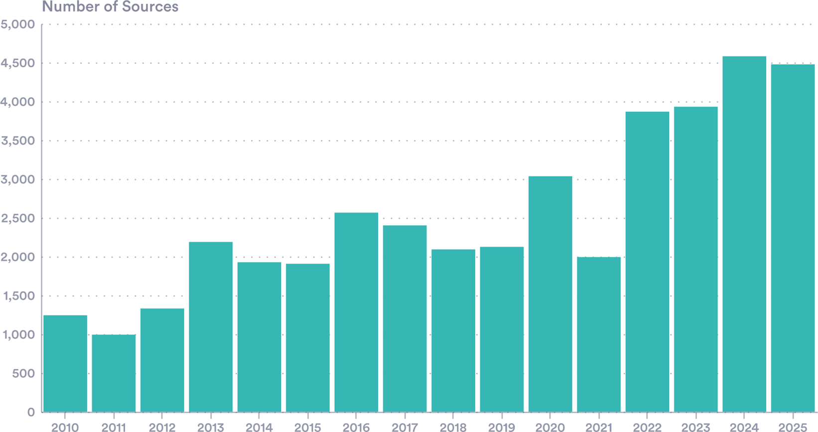
These IFIs have come to play a major role in the public discussion of fiscal challenges. Their coverage in news media has risen considerably (Figure 11). In the United Kingdom, media mentions of the OBR have increased markedly in recent years and are now triple the levels in 2010, when the OBR was created.
OBR news mentions of ‘OBR’ or ‘Office for Budget Responsibility’ in UK news sources.
Source: Authors’ calculations with Nexis (2025) data.
Note: Mentions in headlines or lead paragraphs only.

Figure 11. Long description
The Y-axis is labeled Number of Sources with increments of 500 from 0 to 5,000. The X-axis lists years from 2010 to 2025. The teal bars show the following approximate values:
* 2010: 1,250
* 2011: 1,000
* 2012: 1,350
* 2013: 2,200
* 2014: 1,950
* 2015: 1,900
* 2016: 2,600
* 2017: 2,400
* 2018: 2,100
* 2019: 2,150
* 2020: 3,050
* 2021: 2,000
* 2022: 3,900
* 2023: 3,950
* 2024: 4,600
* 2025: 4,500
The data shows a general upward trend with significant peaks in 2016, 2020, and a sharp sustained increase starting in 2022.
An important part of IFIs roles is now forecasting: more than 60% of IFIs engage in long-run fiscal analysis, with almost 80% undertaking forecast assessment. This independent analysis often includes estimates of long-run productivity, a vital element in the consideration of fiscal sustainability (Alonso et al., Reference Alonso, Arroyo, Aydin, Balasundharam, Davoodi, Hegab, Lam, Nguyen, Ferro, Sher, Solovyeva and Tchelishvili2025).
There is a strong overlap between these variables used in IFI forecasts, and those needed in the models used by market participant to price and trade sovereign debt (see Section 3). In this sense, IFIs are sources of market news, which are relevant for bond investors. This means that the 2020–2025 debt build-up is new not only in scale but also in the extent to which it is being publicly analysed by independent economists whose forecasts are potentially market moving. Like the other trends above, this may have yield implications, which have been largely unexplored.
3. Prices and yields
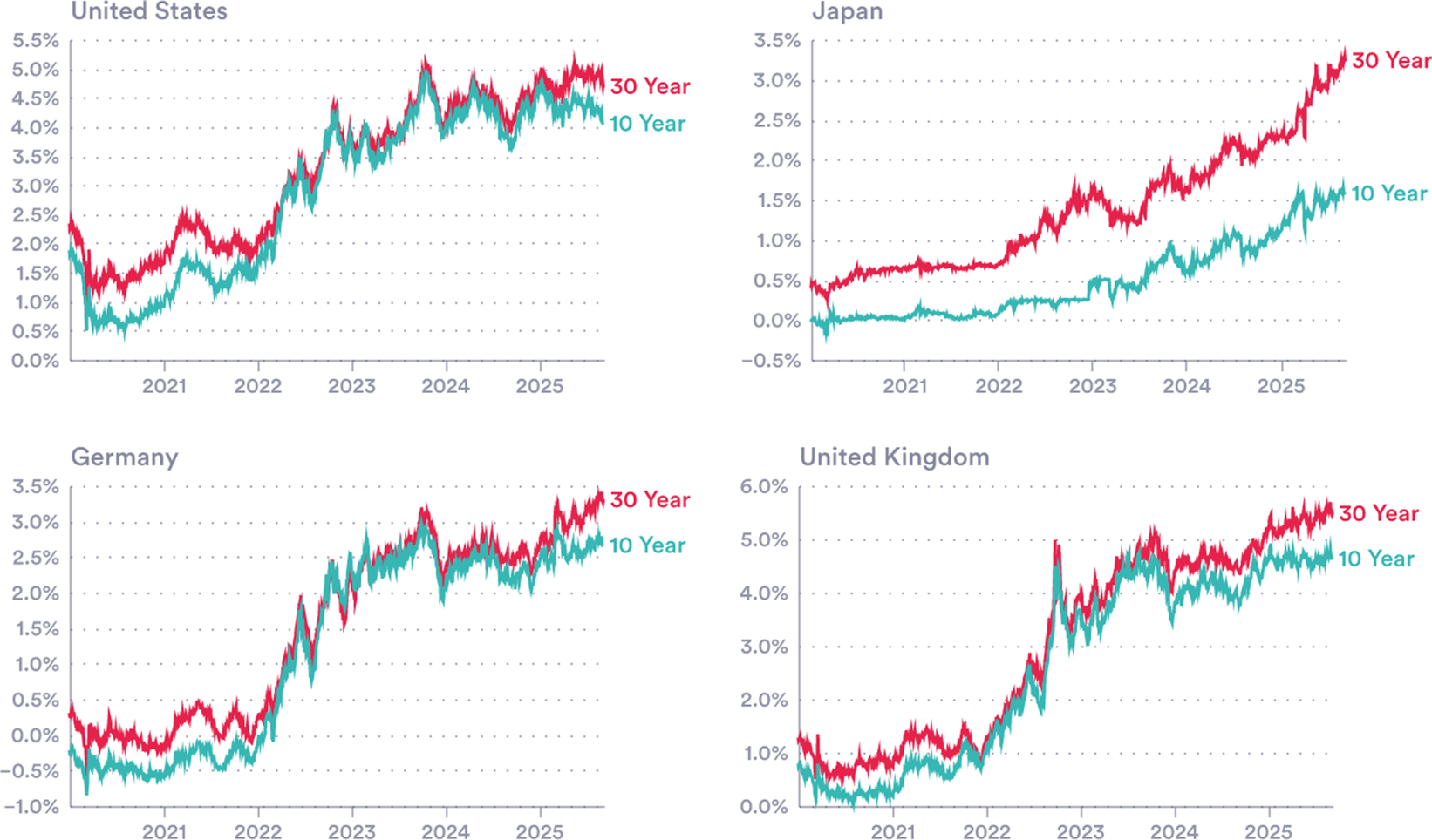
Sovereign borrowing costs in major economies have risen markedly over the past 5 years (Figure 12). Some of this is driven by a general upward shift in yield curves due to higher central bank rates. However, the correlation between policy rates (i.e. central bank rates) and market rates (10- and 30-year bond rates) has been low in recent years (see Section 1). This indicates that other factors may be driving yields, including those set out above. This section examines these forces looking at domestic and international explanations.
Rising yields. 10- and 30-year bond yields in four G7 countries.
Sources: National sources via LSEG Workspace.
Note: Y-axis scales differ from chart-to-chart. A full G7 panel is presented in Figure 7 (Supplementary Material).

Figure 12. Long description
A four-panel line graph displays bond yields for four G 7 countries. Each panel features a horizontal x-axis representing years from 2021 to 2025 and a vertical y-axis representing yield percentages. Two lines are plotted in each: a red line for 30 Year yields and a teal line for 10 Year yields.
* Top-Left Panel, United States: Y-axis ranges from 0.0 percent to 5.5 percent. Both yields start near 1.0 to 2.0 percent in 2021, showing a sharp upward trend through 2022 and 2023, peaking near 5.0 percent in late 2024 before a slight plateau.
* Top-Right Panel, Japan: Y-axis ranges from minus 0.5 percent to 3.5 percent. Yields remain very low and flat near 0.0 percent until 2023. From 2023 to 2025, both lines show a steady, significant increase, with the 30 Year yield reaching over 3.0 percent and the 10 Year yield reaching approximately 1.5 percent.
* Bottom-Left Panel, Germany: Y-axis ranges from minus 1.0 percent to 3.5 percent. Yields start in negative territory in 2021. They rise sharply throughout 2022, fluctuating between 2.0 percent and 3.0 percent through 2024 and 2025.
* Bottom-Right Panel, United Kingdom: Y-axis ranges from 0.0 percent to 6.0 percent. Yields start below 1.5 percent in 2021. There is a volatile but steep climb starting in 2022, with a notable spike in late 2022. By 2025, the 30 Year yield fluctuates near 5.5 percent and the 10 Year yield near 4.5 percent.
In all panels, the 30 Year yield consistently remains higher than the 10 Year yield, and all four countries show a general upward trajectory over the five-year period.
3.1. Estimating bond yields
Many market participants use simple macro-financial models, which seek to explain yields with macroeconomic variables including growth, inflation, bond issuance and global spillovers.Footnote 10 We estimate a simple and widely used model of this kind, incorporating inflation and interest rate expectations.Footnote 11
Our work relates to other analyses of unexplained bond market behaviour. Lizardo and Mollick (Reference Lizardo and Mollick2011) find that Chinese purchases of US debt significantly lowered and flattened the US Treasury yield curve during the Greenspan Conundrum period. Wolcott (Reference Wolcott2020) demonstrates that foreign official purchases primarily depressed medium-term yields despite conventional focus on the long end of the curve.
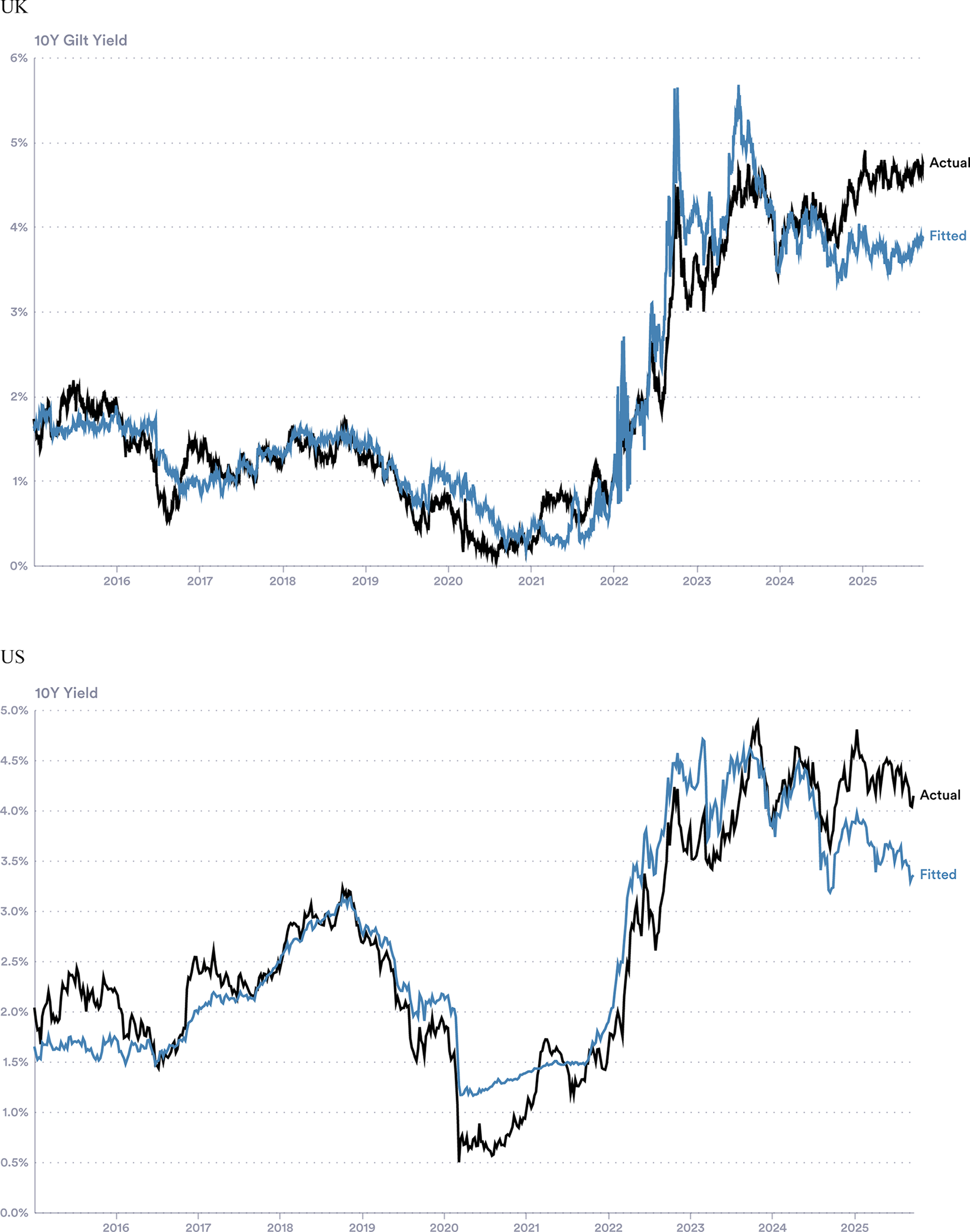
First, we ask whether a minimal expectations-based model can explain observed movements in bond yields. We regress US and UK 10-year yields on inflation expectations (10-year averages derived from inflation-indexed bond spreads) and expected policy rates (1-year-ahead expectations derived from futures), using weekly data from January 2015 to October 2025. Modelled and observed yields are presented in Figure 13.
Full-sample fair-value model for the UK and US. Actual and fitted 10-year yields.
Source: Authors’ calculations using 10-year breakeven inflation (FRED, US and LSEG workspace, UK) and rate expectations (CME via LSEG Workspace, United States; 1 year SONIA-implied rates, UK).
Notes: Regressed with weekly data 2015–October 2025.

Figure 13. Long description
The image consists of two vertically stacked line graphs.
Top Panel: U K 10 Y Gilt Yield.
* The y-axis ranges from 0 percent to 6 percent. The x-axis spans from 2015 to late 2025.
* A black line represents Actual data and a blue line represents Fitted data.
* From 2015 to 2022, both lines fluctuate between 0 percent and 2 percent, showing a high degree of correlation.
* In 2022, both lines spike sharply upward. The Actual line peaks near 4.5 percent while the Fitted line shows a higher, more volatile spike reaching nearly 6 percent.
* By 2025, the Actual line stabilizes around 4.5 percent, while the Fitted line trends lower, ending near 4 percent.
Bottom Panel: U S 10 Y Yield.
* The y-axis ranges from 0.0 percent to 5.0 percent. The x-axis spans from 2015 to late 2025.
* From 2015 to 2019, yields fluctuate between 1.5 percent and 3.5 percent.
* In early 2020, both lines drop sharply, with the Actual black line hitting a trough near 0.5 percent while the Fitted blue line remains slightly higher near 1.2 percent.
* Starting in 2022, both lines rise steeply. The Actual line peaks near 5 percent in late 2023.
* Toward 2025, the Actual line remains elevated above 4 percent, while the Fitted blue line diverges downward, ending near 3.5 percent.
The simple model accounts for approximately 91% and 87% of the variation in the United Kingdom and the United States, respectively, 10-year yields over this period. According to this simple construction, a one-percentage-point increase in expected policy rates is associated with a 0.83 (United Kingdom) and 0.63 (United States) percentage point increase in current yields. A one-percentage-point increase in average 10-year inflation expectations is associated with a 0.20 percentage point increase in the United States, but a negligible increase in the United Kingdom, consistent with its effect being largely absorbed by closely correlated rate expectations.
However, in recent years, a gap emerges between model-implied and observed yields. The fundamental-based fitted values consistently fall short of realised 10-year yields (Figure 13). We see a similar pattern in the United Kingdom. Despite well-anchored inflation expectations and markets pricing policy easing, 10-year observed yields were around 0.8 percentage points higher in the United States and 0.86 higher in the United Kingdom than implied by the model at the start of October 2025. This suggests that some structural determinant of these long-term yields has changed.
While the UK evidence confirms the presence of a similar divergence to the United States, data limitations constrain the range of potential explanatory variables. In this first look at new factors, we therefore focus on the United States in what follows, where richer data allow a more detailed examination of how bond pricing relationships may have changed.
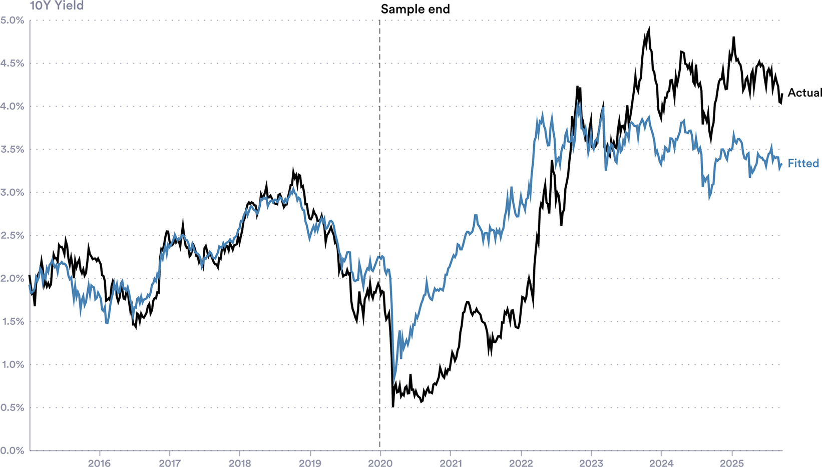
In a similar exercise, we ask whether the past 5 years have seen a shift in bond yield determinants. To evaluate recent yields against pricing relationships that prevailed earlier, we follow Wolcott (Reference Wolcott2020) and Lizardo and Mollick (Reference Lizardo and Mollick2011) and use yields fitted from a restricted sample. In this specification, we restrict our sample to weekly observations ending in December 2019, in essence asking how a bond market participant with this information would view 2020 onwards.
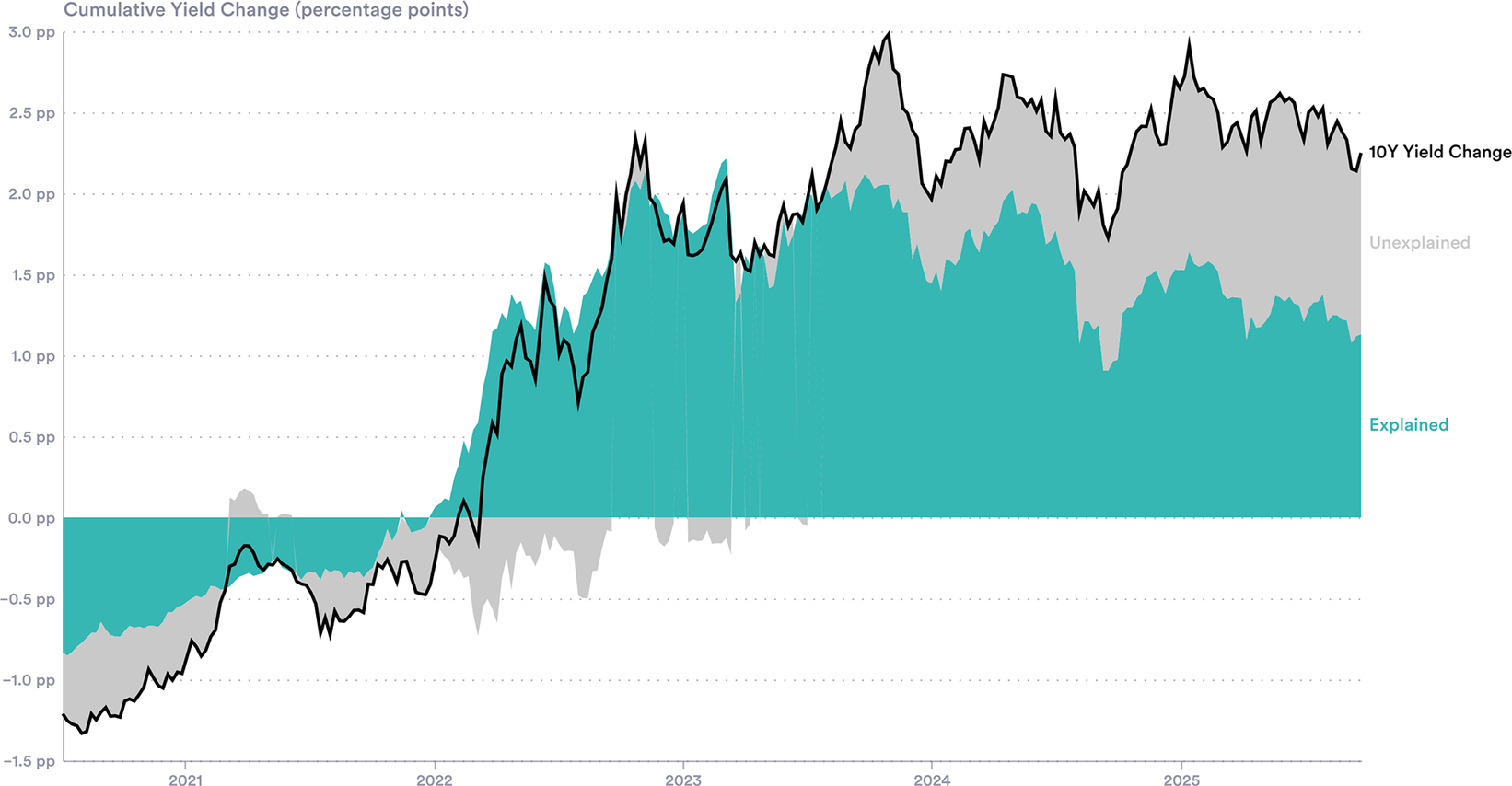
In the restricted-sample specification, the gap between fitted and observed yields remains: there are periods when yields appear both too low (2021 and 2022) and too high (2024 onwards) compared to historical patterns (Figure 14). Full coefficients are reported in Table 2 in the Supplementary Material. By October 2025, this gap is approximately 0.8 percentage points, virtually identical to that obtained from the full-sample specification. Cumulatively, 10-year yields rose by 2.25 percentage points between July 2020 and October 2025, of which the fair-value model accounts for approximately 1.13 percentage points, leaving roughly half of the increase unexplained (Figure 15).
Restricted-sample fair-value model for the US. Actual and fitted 10-year US yields.
Source: Authors’ calculations using 10 year breakeven inflation (FRED) and 1 year Fed rate expectations (CME via LSEG Workspace).
Note: Regressed with weekly data 2015–end of 2019.

Figure 14. Long description
A line graph with the y-axis labeled 10 Y Yield ranging from 0.0 percent to 5.0 percent in 0.5 percent increments. The x-axis represents years from 2015 to 2025. A vertical dashed line labeled Sample end is positioned at the start of 2020.
* From 2015 to the end of 2019, the black line labeled Actual and the blue line labeled Fitted track each other very closely, fluctuating between 1.5 percent and 3.0 percent.
* Following the Sample end line in early 2020, both lines drop sharply toward 0.5 percent.
* From mid-2020 onward, the lines diverge. The blue Fitted line shows a steady upward trend, reaching approximately 3.5 percent by 2025.
* The black Actual line remains lower than the fitted model through 2021, then rises much more aggressively, peaking near 5.0 percent in late 2023 before settling around 4.0 percent in 2025.
* The gap between the Actual and Fitted lines is most pronounced between 2022 and 2025.
Yield change decomposition. Cumulative contribution to the change in yields since July 2020, according to our fair value model.
Source: Authors’ calculations using 10-year yields.
Note: Regressed with weekly data, 2015–2019.

Figure 15. Long description
The vertical Y axis measures Cumulative Yield Change in percentage points (p p) ranging from minus 1.5 p p to 3.0 p p in 0.5 p p increments. The horizontal X axis represents time from early 2021 to early 2025.
Three data series are presented:
1. A solid black line labeled 10 Y Yield Change tracks the total cumulative change. It starts at approximately minus 1.2 p p in 2021, crosses the 0.0 p p baseline in early 2022, peaks near 3.0 p p in late 2023, and ends near 2.2 p p in 2025.
2. A teal shaded area labeled Explained represents the portion of the change accounted for by the model. This area remains below the baseline until early 2022, then rises steadily to peak around 2.0 p p in late 2023 before settling near 1.2 p p by 2025.
3. A light gray shaded area labeled Unexplained represents the residual difference between the black line and the teal area. This gap is narrow in 2021 and 2022 but widens significantly from 2024 onwards, indicating that a larger portion of the yield change is not captured by the model's explained variables in the later period.
A natural question is whether this change in structure reflects instability in the expectations-based relationship, or instead the emerging importance of factors outside the model. While estimated coefficients do change across samples, the persistence and similar magnitude of the resulting gap point to the importance of factors omitted from the expectations-based framework.
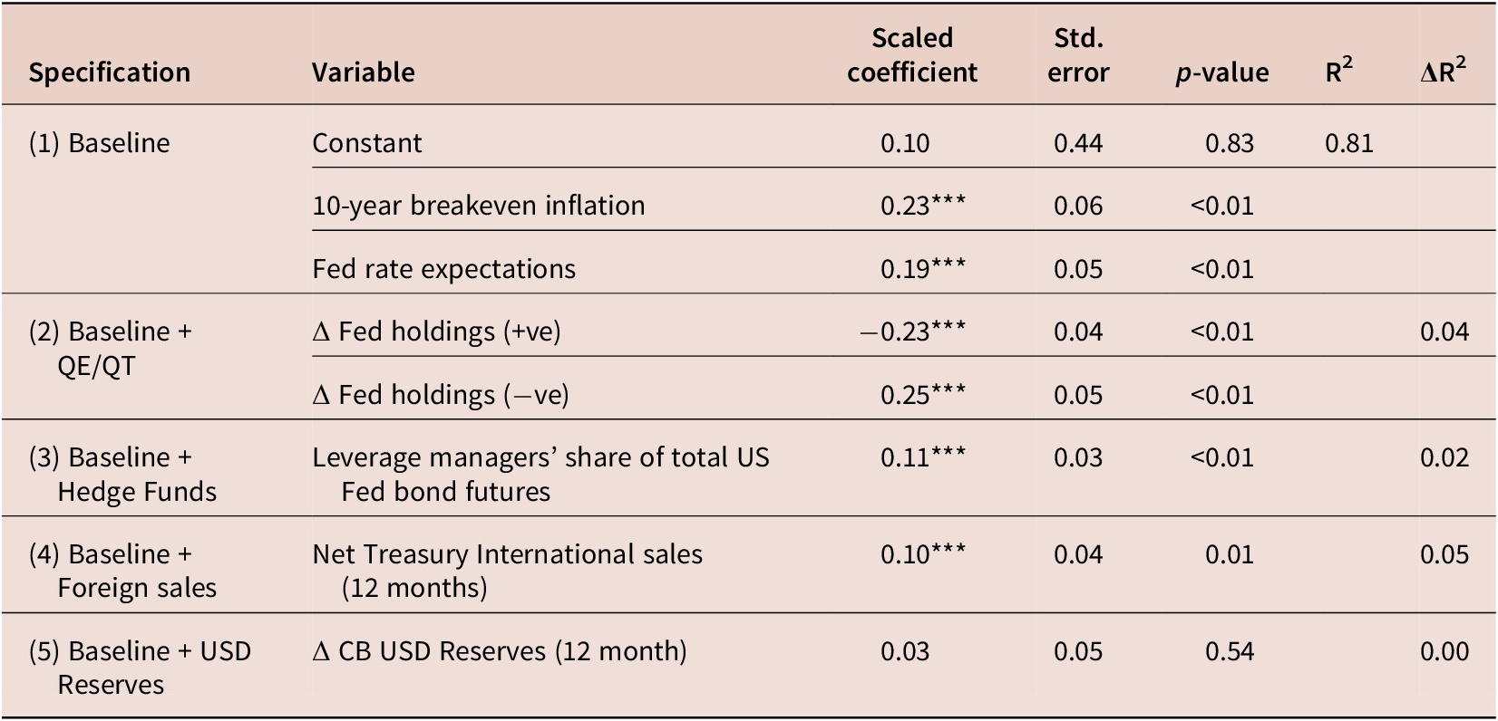
Motivated by our discussion of market evolution above, we next augment the baseline model with four additional regressors in an attempt to understand new determinants of bond yields (Table 1). Each factor is entered separately into the base specification. This section focuses on the United States, due to current data availability. These factors are as follows:
-
• Reserve accumulation: central bank reserves of US dollars from the IMF COFER (2025) database.
-
• Foreign holdings: net sales of US Treasury bonds to the rest of the world.
-
• Hedge funds: leveraged money manager’s share of total US 10-year bond futures (CFTC, 2025).
-
• Quantitative easing/tightening: changes in US Federal Reserve holdings of US Treasury Securities (FRED: TREAST, 2025). We allow for asymmetric effects of QE/QT with separate regressors for 12-month positive and negative changes.
Exploratory yield regressions

Table 1. Long description
The table contains seven columns: Specification, Variable, Scaled coefficient, Std. error, p-value, R super 2, and Delta R super 2.
* Specification 1 (Baseline): Constant has a coefficient of 0.10 (p-value 0.83). 10-year breakeven inflation has a coefficient of 0.23 (p-value < 0.01). Fed rate expectations has a coefficient of 0.19 (p-value < 0.01). The R super 2 for this model is 0.81.
* Specification 2 (Baseline plus Q E / Q T): Delta Fed holdings (positive) has a coefficient of minus 0.23 (p-value < 0.01). Delta Fed holdings (negative) has a coefficient of 0.25 (p-value < 0.01). The Delta R super 2 is 0.04.
* Specification 3 (Baseline plus Hedge Funds): Leverage managers’ share of total U S Fed bond futures has a coefficient of 0.11 (p-value < 0.01). The Delta R super 2 is 0.02.
* Specification 4 (Baseline plus Foreign sales): Net Treasury International sales (12 months) has a coefficient of 0.10 (p-value 0.01). The Delta R super 2 is 0.05.
* Specification 5 (Baseline plus U S D Reserves): Delta C B U S D Reserves (12 month) has a coefficient of 0.03 (p-value 0.54). The Delta R super 2 is 0.00.
Note: Triple asterisks denote statistical significance at the 0.01 level. Standard errors are H A C-robust.
Note: Weekly data. Baseline model includes 1 Y forward rate expectations and 10 Y breakeven inflation. All augmented regressors are standardised. ** p < 0.01, * p < 0.05. Standard errors are HAC-robust with five lags.
This preliminary analysis is highly stylised, with causal links needing deeper investigation. However, some interesting patterns appear.
-
• Quantitative easing/tightening. QE and QT show expected directional associations with yields: balance sheet expansions (QE) correlate with yield decreases (β = −0.23, p < 0.01), while contractions (QT) correlate with increases (β = 0.25, p < 0.01). The magnitudes are roughly symmetric: a 1 SD deviation change in holdings ($41 billion over 12 months during January 2015–December 2019) associates with a 23–25 basis point movement.
-
• Hedge funds. Leverage managers’ share of total futures positioning correlates with yields (β = 0.11, p < 0.01) but explains limited additional variation (ΔR2 = 0.02). The direction is consistent with the ‘basis trade’ channel.
-
• Foreign sales. Net international sales of US Treasuries show a strong pattern. The direction suggests that periods of higher foreign buying are associated with higher yields, consistent with demand-inducing effects of higher returns. This relationship may therefore capture foreign participants responding to yield changes rather than driving them.
-
• Reserve accumulation. The lagged change in foreign central bank’s USD reserves shows no detectable association with yields. Despite the documented decline in dollar-denominated reserves, this diversification does not correlate with US borrowing costs in our sample.
Taken together, these indicative relationships point to stronger domestic drivers (Central Banks, hedge funds) than foreign ones. Clearly, however, deeper research is needed: although several coefficients are statistically significant, their explanatory power means much of the unexplained variation in bond yields remains.
We now turn to two more factors—UN demographics downgrades, and peak activity periods of fiscal watchdogs—which have both been posited as a potential influence on bond markets.
3.2. Demographic projections
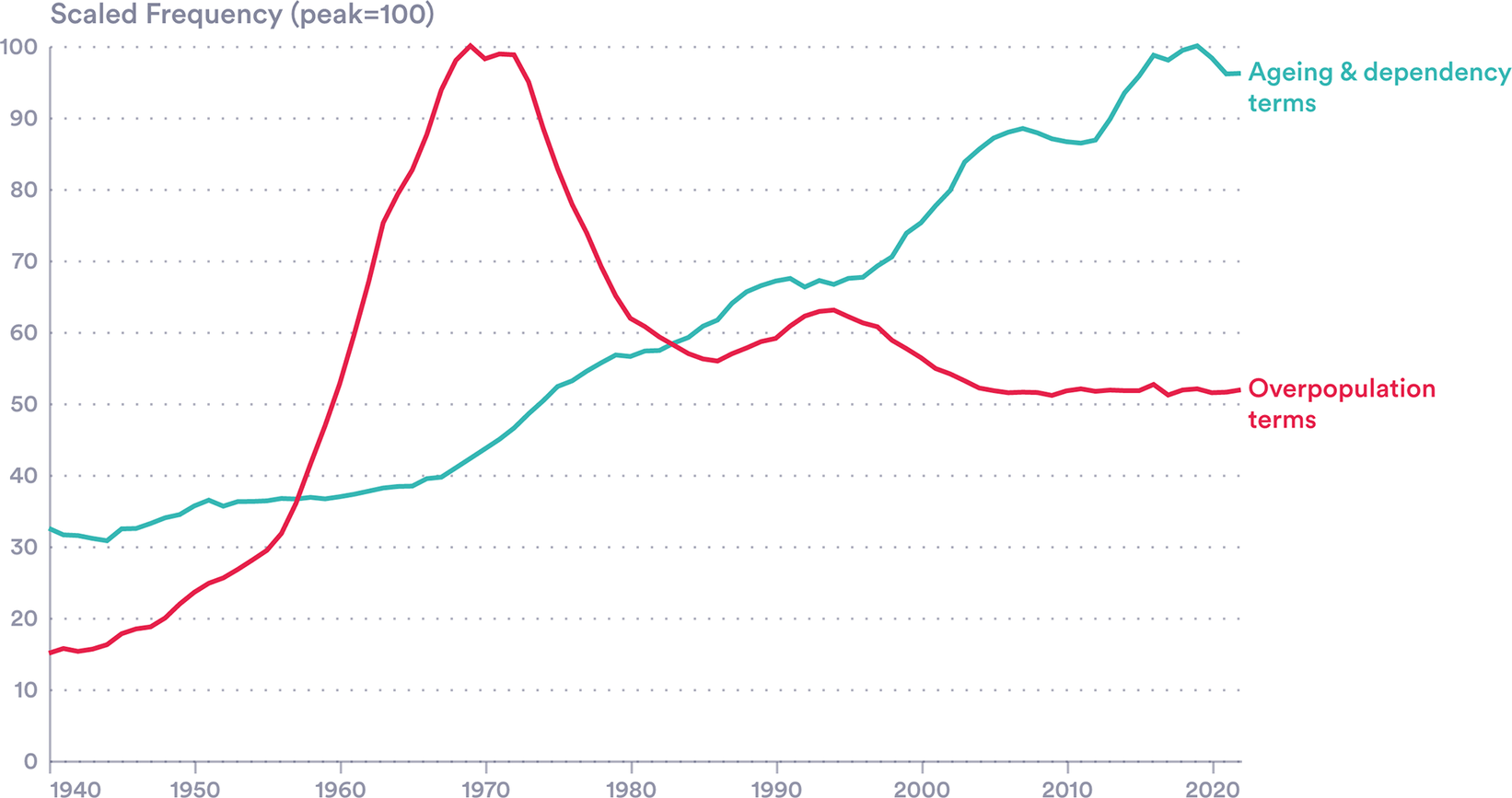
The salience and tenor of demographic concerns have changed over the past 40 years. The Malthusian worry of overpopulation has been replaced in the 21st century by fears of a slowing and top-heavy population distribution: more ageing and, in most advanced economies, fewer births than deaths. The shift is visible in policy: in South Korea, China, India and Japan, anti-natalist policies including one-child restrictions are starting to be replaced by pro-natalist incentives. It is also visible in the literature: mentions of overpopulation-related terms peaked in the early 1970s, while concern over dependency is still growing (Figure 16).
Demographic salience. Google Ngram results for terms associated with concerns with overpopulation and ageing population.
Note: Separate Google Ngram queries for terms associated with ageing and dependency, and overpopulation, concerns, were performed, aggregated, and normalised to the peak year = 100.
Ageing/demographic decline terms: aging/ageing population; population aging/ageing; demographic decline; population decline; declining population; depopulation; low fertility; falling fertility; declining birth rate; below-replacement fertility; replacement fertility; shrinking population; population shrinkage; baby bust; birth dearth.
Overpopulation terms: overpopulation; population explosion; population bomb; rapid population growth; runaway population growth.
Source: Authors’ calculations using the Google Books Ngram Viewer (English corpus), first described in Michel et al. (Reference Michel, Shen, Aiden, Veres, Gray, Brockman, Pickett, Hoiberg, Clancy, Norvig, Orwant, Pinker, Nowak and Aiden2011).

Figure 16. Long description
The X-axis represents years from 1940 to 2020 in 10-year increments. The Y-axis represents Scaled Frequency (peak equals 100) with horizontal grid lines at intervals of 10. Two lines are plotted:
* Overpopulation terms (red line): Starts at approximately 15 in 1940. It rises sharply beginning in the late 1950s, reaching a sharp peak of 100 around 1970. Following this peak, it declines rapidly until 1985, then experiences a minor secondary rise to about 63 in the mid-1990s before plateauing and slightly declining to approximately 52 by 2020.
* Ageing and dependency terms (teal line): Starts at approximately 32 in 1940. It remains relatively flat until 1965, then begins a steady, long-term upward climb. It intersects the declining red line around 1983 at a value of 58. The teal line continues to rise, reaching its peak of 100 around 2015, before ending at approximately 96 in 2020.
By the end of the period, the frequency of ageing and dependency terms is nearly double that of overpopulation terms.
Despite the fact that population decline is well known, its rate is still delivering shocks that should be relevant for bond markets. As we show in Section 2, fertility forecasts have not only just been weak but also wrongly optimistic (Figure 10). With each edition of the World Population Prospects since 2010, the UN has downgraded its fertility projections.
There are long-run implications. Revisions to annual fertility rates build over time. Sovereign bonds today are being issued at 30+ year durations, set to mature as the cost of contemporary low fertility is felt, in labour force terms. Declining fertility rates today have a staggered and delayed fiscal impact due to the U-shaped age dependency profile: in the short-run, lower fertility can mean lower government expenditure (nurseries, schools) with the cost borne 2–3 decades later as the (significantly smaller) cohorts born today enter the workforce. In advanced economies, the impact of record-low fertility will arrive just as record-high issuance of debt matures.
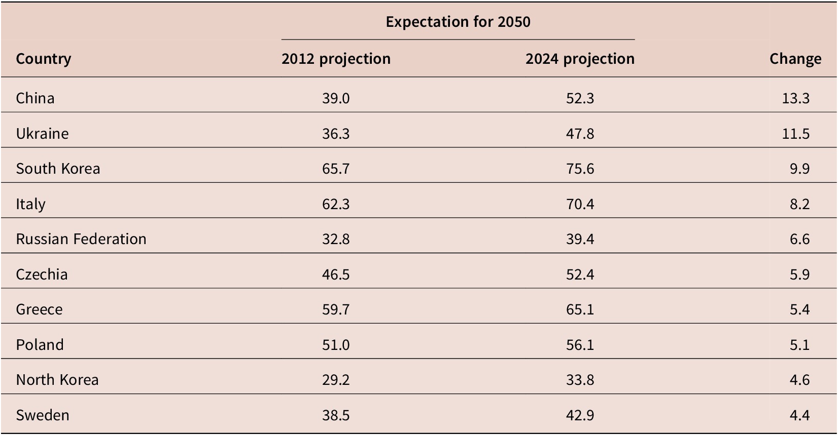
The magnitudes of revisions vary by country (Table 2). While fertility projections have been near-universally lowered, old-age dependency—the number of people 65+ per those 15–64 is also sensitive to migration estimates and is more mixed: some countries that have seen increased migration have seen smaller or positive modifications to projections. The countries that have seen the largest increases in expected dependency include a number of G7 and G20 economies. Of particular note:
-
• South Korea and China, where anti-natalist policies accompanied a swing from high to sub-replacement fertility.
-
• Italy, which is rapidly ageing, and has seen declining, though still positive, net migration.
-
• Ukraine, with a war-demographic crisis of conflict fatality and refugee outflows.
-
• Russia, with both a low fertility rate and reduced migration.
Largest upwards revisions to old-age dependency expectations for 2025

Table 2. Long description
The table consists of four columns: Country, 2012 projection, 2024 projection, and Change. The data represents expectations for the year 2050.
* China: 2012 projection 39.0, 2024 projection 52.3, Change 13.3.
* Ukraine: 2012 projection 36.3, 2024 projection 47.8, Change 11.5.
* South Korea: 2012 projection 65.7, 2024 projection 75.6, Change 9.9.
* Italy: 2012 projection 62.3, 2024 projection 70.4, Change 8.2.
* Russian Federation: 2012 projection 32.8, 2024 projection 39.4, Change 6.6.
* Czechia: 2012 projection 46.5, 2024 projection 52.4, Change 5.9.
* Greece: 2012 projection 59.7, 2024 projection 65.1, Change 5.4.
* Poland: 2012 projection 51.0, 2024 projection 56.1, Change 5.1.
* North Korea: 2012 projection 29.2, 2024 projection 33.8, Change 4.6.
* Sweden: 2012 projection 38.5, 2024 projection 42.9, Change 4.4.
Source: Authors’ calculations using U N W P P 2013 and U N W P P 2024. Note: Includes countries with populations of at least 10 M in 2024.
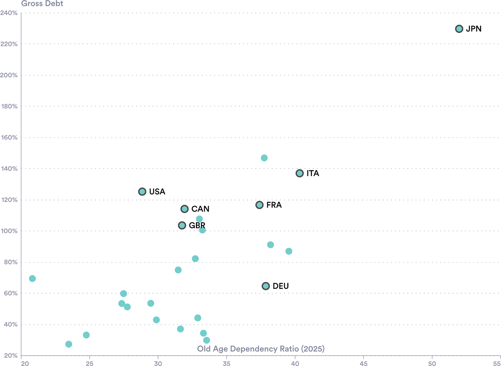
The countries with the highest dependence ratios are also those with the highest current debt. Japan, furthest along this path, has both the highest relative debt burden and the largest old age dependency ratio of any OECD advanced economy (Figure 17). Italy has similar characteristics, with the rest of the G7 close behind. The concern is that those countries which are set to be affected most by the burden of an ageing population are also those with the least fiscal room to meet the challenge.
High dependency, high debt. Public debt and old-age-dependence for OECD advanced economies.
Source: UN WPP (2024) and OECD (2025).
Note: Public sector debt at the end of 2024 and estimated old age dependency ratio in 2025.

Figure 17. Long description
A scatter plot with the horizontal X axis representing the Old Age Dependency Ratio 2025, ranging from 20 to 55. The vertical Y axis represents Gross Debt as a percentage, ranging from 20 percent to 240 percent.
Most data points are clustered in the lower-left quadrant, between a dependency ratio of 20 to 35 and debt levels of 20 percent to 80 percent.
Key labeled outliers include:
* U S A at approximately 29 dependency and 125 percent debt.
* C A N at 32 dependency and 115 percent debt.
* G B R at 32 dependency and 105 percent debt.
* F R A at 37 dependency and 118 percent debt.
* I T A at 40 dependency and 138 percent debt.
* D E U at 38 dependency and 65 percent debt.
* J P N is the extreme outlier in the top-right corner at approximately 52 dependency and 230 percent debt.
All this adds up to a fiscal risk. The question is how much of this is being acknowledged by bond markets and the extent to which it might explain the level and volatility of bond yields. As a simple first test as to whether bond markets respond to new demographic information, we examine yield movements around the release dates of UN World Population Prospects revisions since 2008. We use a simple event study approach with windows spanning 2 days and 6 weeks post-release, to capture immediate and delayed market reactions. We find no consistent or discernible relationship between changes in 30-year bond yields or the 30 Y–10 Y term spread, against the magnitude of demographic revisions (measured by changes in projected old-age dependency ratios) with each release.
We also look at whether age helps in simple bond yield models. Again, no consistent relationship appears. In fact, the simple correlation between old-age dependency and yields today is weakly positive among OECD countries, likely confounded by the wealthier countries that both aged earlier and command lower borrowing costs as a result of perceived creditworthiness. Looking instead at expected increases in the dependency ratio has the same result.
Taken together, these results suggest UN demographic data play little role in bond yields. One explanation is pre-emption: markets may have earlier and more direct data, perhaps from individual nations’ census offices. Another would be discount rates: demographic impacts are further into the future than the host of other factors that markets must weigh, with their impact shrunk by the reverse-telescope of discounting. This is an area for fiscal authorities to watch, since dependency is growing, with certainty, and there are fiscal implications. A period of gradual market adjustment would be easier to manage than a sudden revision.
3.3. Fiscal watchdogs prominence
In this section, we propose a new bond market test: asking whether UK gilt yields respond systematically to Office for Budget Responsibility (OBR) activity. This question pre-dates, but was drawn into sharper focus by, the events around the November 2025 UK budget.
IFIs, including the OBR, produce forecasts and assessments that potentially move bond markets. They can provide information in at least two ways: by providing news on fiscal sustainability and by motivating fiscal policy changes from finance ministers guided or constrained by their assessments. To explore this relationship, we have assembled three series, covering the OBR’s inception in 2010 to the present:
-
• News salience. Mentions of the OBR in The Times news headlines and lead paragraphs. From an initial scrape of around 10,000 articles, we identify 445 closely OBR-related items, which cluster into 44 distinct periods of elevated coverage using entry and exit thresholds designed to avoid overlapping events.
-
• Release dates. A comprehensive set of 318 unique OBR publication dates, including Economic and Fiscal Outlooks, Budget analyses, data evaluations and formal statements, and other documents.
-
• Forecast revisions. The direction and magnitude of changes to public sector net borrowing forecasts associated with 30 major OBR forecast releases, constructed by summing revisions across overlapping fiscal years.
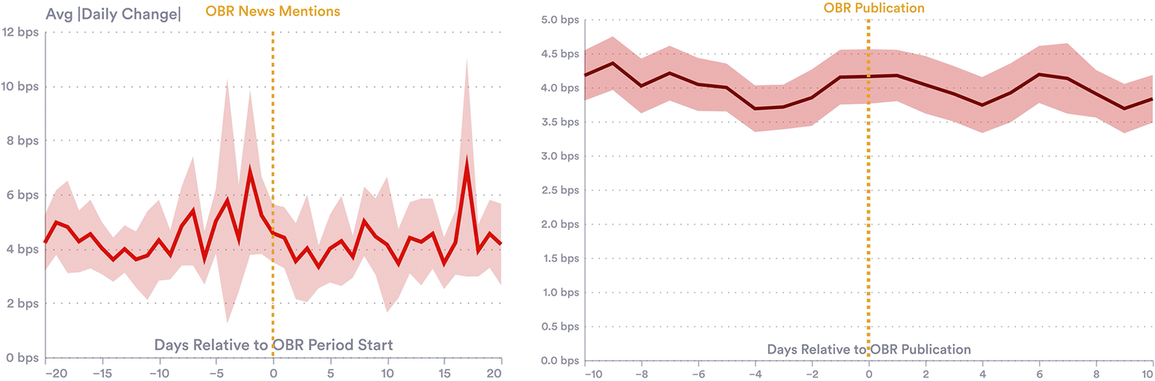
Our findings here suggest that the recent (November 2025) turmoil is rare: OBR outputs appear largely anticipated by markets and absorbed without creating additional volatility. Similarly, we find no evidence that gilt yields are significantly more volatile while salience in news is high. Across specifications examining same-day and next-day movements, directional changes and absolute magnitudes, effects are small and statistically insignificant. While publication dates are associated with a 3–4% increase in daily absolute yield moves (≈0.1–0.2 basis points), this is negligible relative to typical daily volatility (Figure 18).
Yield volatility around OBR events. Yield volatility around heightened OBR news mentions or OBR publications.
Note: Average absolute daily change in UK 10 Y yields in the days before and after OBR publications (right) and periods of heightened media coverage (left), proxied by periods when the OBR is mentioned the headline or lead paragraphs of at least eight articles in The Times, or the 7 day average exceeds four articles.

Figure 18. Long description
A two-panel line graph.
Left Panel: O B R News Mentions.
The y-axis is labeled Avg absolute value Daily Change in b p s, ranging from 0 to 12. The x-axis is labeled Days Relative to O B R Period Start, ranging from minus 20 to 20. A vertical dashed gold line marks day 0. The data shows a volatile red line with a light red shaded confidence interval. Significant spikes occur around day minus 4 and day 17, reaching approximately 7 b p s and 8 b p s respectively. Between these spikes, the yield change fluctuates mostly between 3 and 5 b p s.
Right Panel: O B R Publication.
The y-axis is labeled in b p s, ranging from 0.0 to 5.0. The x-axis is labeled Days Relative to O B R Publication, ranging from minus 10 to 10. A vertical dashed gold line marks day 0. The red line is much smoother than the left panel, hovering consistently between 3.7 and 4.4 b p s. There is a slight peak at day 0 and day 6, with the shaded confidence interval remaining narrow and stable throughout the 20-day period.
Similarly, we find no systematic relationship between the magnitude of OBR forecast revisions and gilt yield movements. That is to say, the change in medium-term expected borrowing is not strongly correlated with the change in yields.
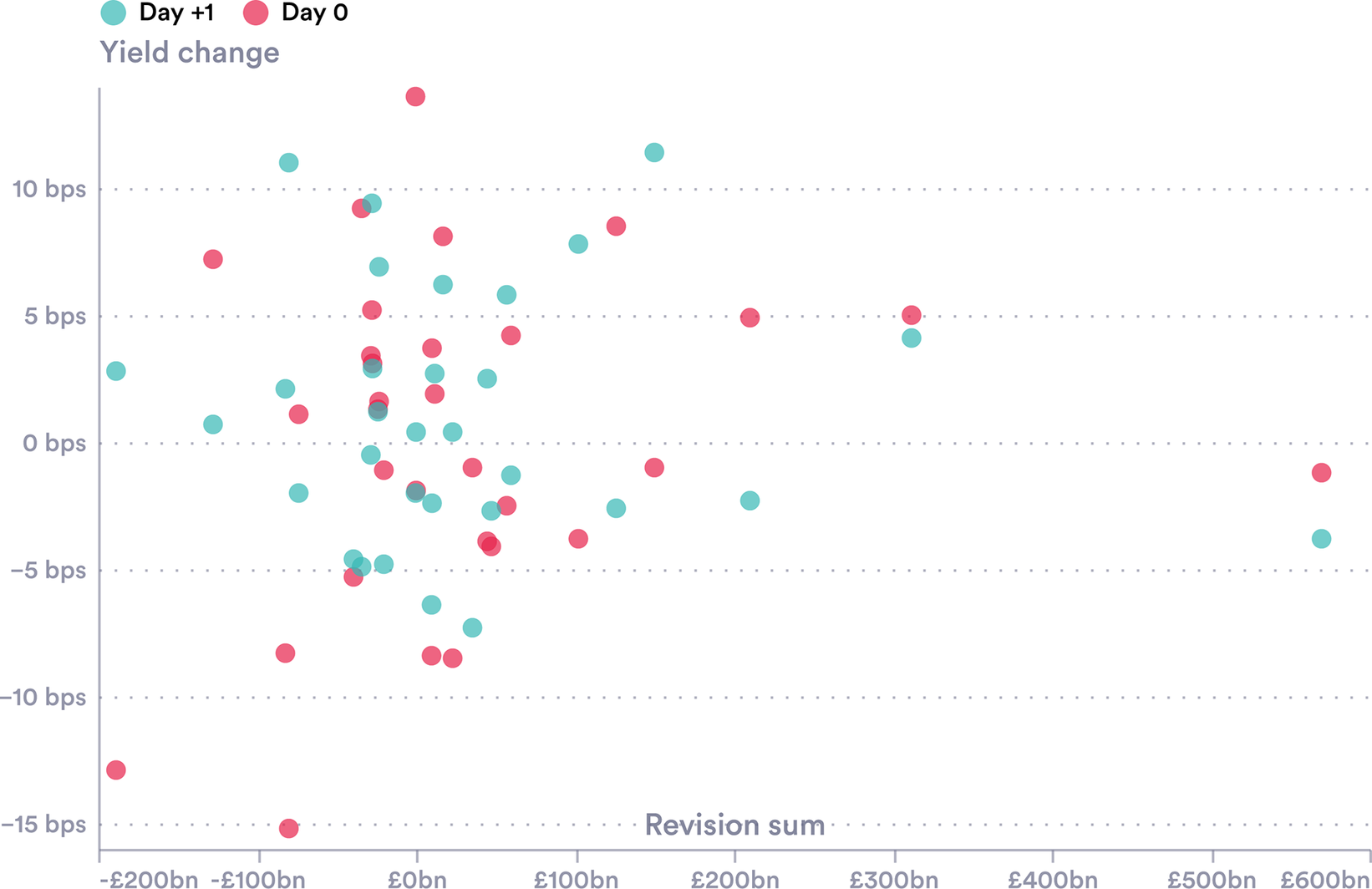
For each OBR publication, we calculate the sum of revisions to public sector net borrowing forecasts across overlapping fiscal years (5–6 years), capturing the magnitude and direction of the revision. Figure 19 plots these revision magnitudes against same-day and next-day yield changes. The scatter shows no discernible pattern: large upward revisions (indicating worse fiscal outlook) do not consistently associate with yield increases, nor do large downward revisions associate with decreases. Calculated correlations are weak and a small sample size (30 complete forecast publication dates since 2010) constraints statistical power.
Forecast revisions and yield changes. Cumulative borrowing forecast revisions versus gilt yield changes.
Note: Changes in UK 10 Y yields on the day of and day after OBR forecast publications, plotted against the size of revisions.

Figure 19. Long description
A scatter plot with two data series. The horizontal X axis is labeled Revision sum and ranges from minus £200bn to £600bn in increments of £100bn. The vertical Y axis is labeled Yield change and ranges from minus 15 b p s to 10 b p s in increments of 5 b p s. A legend at the top identifies two categories: Day 0 represented by pink dots and Day +1 represented by teal dots.
* The majority of data points are clustered between minus £100bn and £100bn on the X axis and between minus 10 b p s and 10 b p s on the Y axis.
* There is no clear linear correlation between the size of the revision and the yield change, as points are widely dispersed vertically around the 0 b p s line.
* Outliers include a significant positive revision near £600bn with a yield change between 0 and minus 5 b p s, and a negative revision near minus £200bn with a yield change below minus 10 b p s.
* Horizontal dotted grid lines mark every 5 b p s interval on the Y axis.
We share these null findings and accompanying datasets to help stimulate future research. This idea, which developed during the course of writing this paper, has become particularly important given the events of Q4 2025—see, for example, OBR (2025) and recent parliamentary debates (Hansard, 2025). The complete datasets, with scraped news mentions, publication dates and calculated forecast revisions, are available with this paper.Footnote 12
4. Conclusion
This paper examines whether the fiscal constraint posed by bond markets in advanced economies is changing, by examining the forces driving bond yields. The evidence presented suggests significant change: the scale of G7 debt, the players involved and the behaviour of yields—both levels and volatility—suggest this is a vital area of research.
We present several stylised facts. First, the scale of borrowing is new; debt-to-GDP ratios now average 110%, compared to 85% two decades ago. Second, the composition of bond holders has shifted with central bank holdings starting to fall after the 2008 and 2020 surges. While foreign holdings have fallen as a share of total debt, non-bank financial institutions have become major players. Third, long-dated yields have risen sharply since 2020, with increases ranging from 1.6 percentage points in Japan to 4.8 percentage points for UK 30-year gilts.
Simple macro-financial models that performed reasonably before 2022 currently leave substantial variation unexplained. Our exploratory analysis examines several structural factors. QT shows a clear association with yields. Other factors tested, including the role of hedge fund purchases and foreign reserve strategies, are unclear. Finally, we propose simple, event-study type checks on whether new forms of ‘news’—either from the UN, on demographics, or from fiscal watchdogs, on long-run sustainability, may be having an impact.
This descriptive data analysis outlines a vital area of future research using fuller models and more precise identification strategies. The forces we document suggest the fiscal constraint is evolving in ways that necessitate deeper investigation. Bond markets are a vital source of funding for the kind of long-run investment projects that improve economic outcomes for current generations and those that follow. If they are changing, we need to understand why.
Acknowledgements
The authors are grateful to colleagues at NIESR and in particular Stephen Millard and Adrian Pabst for comments, editing and hosting events that influenced this paper. James Collis helped on an early draft. Samuel Bickel-Barlow, Josh Hellings, Hannah Cantekin and Will Shepherd provided excellent research assistance. All errors, omissions and opinions in this article are our own.
Competing interests
Professor Richard Davies is a member of the Fiscal Policy Panel (FPP) of the States of Jersey. All views in this paper are personal and do not reflect the view of the FPP or its other members.

 Open access

