NOMENCLATURE
- CON
condition
- m
mode number
- N+
positive integer
- P
pressure, Pa
 $\overline{P}$
normalised pressure
- R
rotor
- T
rotor rotation period
- U
blade speed at mean radius, m/s
- V
flow velocity at the inlet, m/s

Greek Symbols
- $\rho$
density, kg/m3
- $\phi$
Vx/U1, flow coefficient
- $\psi$ts
2(Pout-Ptin)/
$\rho$U12, total-to-static pressure rise coefficient- $\Delta\theta$
angular displacement of the two sensors


Subscripts
- 1
front rotor
- 2
rear rotor
- dpl
double-phase-locking
- ens
ensemble-averaged
- in
inlet
- out
outlet
- rms
root-mean-square
- t
total
- x
axial direction
Abbreviations
- BPF
blade passing frequency, Hz
- RI
rotating instability
- RRF
rotor rotating frequency, Hz
- RS
rotating stall
1.0 INTRODUCTION
With the rapid development of aviation technology, higher and higher requirements for engine stability are required. As the two primary flow instability forms, rotating stall (RS) and surge have received widespread attention since the advent of jet engines. After nearly eight decades of unremitting efforts, the understanding of these two types of flow instability has significantly been improved. However, what we know is still very inadequate.
“We can explain what happens when a compressor stalls or surges, but we have little to offer in the way of rigorous rules for designing a more stable compressor”(Reference Day1). Such a situation has led to the growing importance of the active control of compressor flow instability. To get sound control effects, it is especially important to capture the stall warning signal as early as possible(Reference Chen, Johnson, Hathaway and Webster2). With the deepening of the study, it is found that the oscillation of the tip clearance leakage flow often occurs in the pre-stall phase, and may cause the vibration of the rotor blade(Reference Haukap3,Reference Holzinger, Wartzek, Schiffer, Leichtfuss and Nestle4) , which is called rotating instability (RI). It is possible to become a signal for early stall warning.
Mathioudakis and Breugelmans(Reference Mathioudakis and Breugelmans5) first discovered the rotating instability phenomenon by using a hot wire in an axial compressor. At that time, “rotating instability” was not used to describe the phenomenon. To distinguish it from the stall, the former and the latter were respectively called “small stall” and “big stall.” Subsequently, Inoue et al.(Reference Inoue, Kuroumaru, Iwamoto and Ando6) observed the early premature of the stall by installing a high-frequency response pressure sensor on the casing of an axial-flow isolated rotor. The disturbance occurred when the flow rate is higher than the stall point, and it happened only in the large tip or hub clearance(Reference Beselt, Rennings, Thiele and Peitsch7) situations. The phenomenon is rotating instability. Liu et al.(Reference Liu, Holste and Neise8) also observed rotating instability at the non-stall point with large tip clearance. They pointed out that rotating instability is the primary source of tip clearance noise (similar to Fukano et al.(Reference Fukano, Takamatsu and Kodama9–Reference Raitor and Neise11)). Moreover, for the first time, “rotating instability” is used to refer to this phenomenon.
Holste and Neise(Reference Holste and Neise12) arranged the pressure sensors circumferentially on the upstream casing of the rotor. By using the azimuthal mode decomposition techniques, it is found that each peak of the rotating instability band corresponds to a unique dominant circumferential mode. A similar spectral feature was found in the rotating instability of the low-speed axial compressor and the last stage of the steam turbine by Inoue et al.(Reference Inoue, Kuroumaru, Yoshida, Minami, Yamada and Furukawa13) and Zhang et al.(Reference Zhang, He and Ster14) Experiments by Kameier and Neise(Reference Kameier and Neise15,Reference Kameier and Neise16) showed that rotating instability occurred only in the presence of backflow at the rotor tip and exhibited a narrow frequency band below the blade passing frequency. Inoue et al.(Reference Inoue, Kuroumaru, Tanino, Yoshida and Furukawa17) observed that there is a low static pressure zone upstream of the rotor when rotating instability occurred, and it is speculated that the low static pressure zone is caused by the radial vortex attached to the casing. The radial vortex movement in the circumferential direction results in the occurrence of rotating instability. Experiments by Mailach et al.(Reference Mailach, Lehmann and Vogeler18) showed that the interference between the tip clearance vortex and the flow of the adjacent blade passages leads to the occurrence of rotating instability. Marz et al.(Reference Marz, Hah and Neise19) observed that the rotating instability occurs when the tip clearance is large enough, and there was a low static pressure zone moving from the suction side to the pressure side, confirming Inoue et al.’s(Reference Inoue, Kuroumaru, Tanino, Yoshida and Furukawa17) inference.
To explain the physical causes of rotating instability, Pardowitz et al.(Reference Pardowitz, Tapken and Enghardt20) conducted experiments in a circular cascade and proposed a theoretical model that indicates there is an instability wave in the shear layer of the tip clearance region and propagates in the circumferential direction. Since the moment at which these instability waves of different wavelengths appear is random, the rotating instability has stochastic characteristics. A high-speed stereoscopic particle image velocimetry (PIV) was used to detect the rotating instability flow structure in a radial vaneless diffuser by Dazin et al.(Reference Dazin, Cavazzini, Pavesi, Dupont, Coudert, Ardizzon, Caignaert and Bois21). Pardowitz et al.(Reference Pardowitz, Tapken, Sorge, Thamsen and Enghardt22) used the PIV technique and pressure sensors to capture the instability flow field structure and the corresponding pressure wave when the rotating instability occurred in the annular cascade. By analyzing the correlation between the flow field and the rotational pressure wave, it is confirmed that the instability of the shear layer caused the occurrence of rotating instability. To further test the applicability of the model, Pardowitz et al.(Reference Pardowitz, Tapken, Neuhaus and Enghardt23,Reference Pardowitz, Peter, Tapken, Thamsen and Enghardt24) conducted a verification experiment in an axial fan. The results showed that the rotating instability waves of different wavelengths in the shear layer had a stochastic behavior, and this phenomenon was caused by the backflow in the tip clearance region.
So far, a deep understanding of the rotating instability phenomenon in the conventional (stator-rotor) axial compressor is established. However, as a new aerodynamic layout with bright prospects, in the contra-rotating (rotor-rotor) compressor, the phenomenon of rotating instability has not caused widespread concern. Due to the significant rotor-rotor interference effect in the contra-rotating compressor, the onset of rotating instability could be different from the one in a conventional compressor. To study the rotating instability in the contra-rotating compressor, the author first verifies the effectiveness of the original modal estimation method mentioned in the literature(Reference Kameier and Neise16), and then optimises the method further to improve the numerical accuracy of the modal estimation method. This method significantly reduced the number of pressure monitoring points required for mode analysis and thus has a total application value in engineering.
2.0 EXPERIMENTAL SETUP
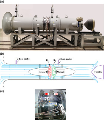
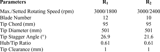
The experiment was carried out on a test bench for a contra-rotating axial flow compressor (shown as Fig. 1), and the detailed design parameters are shown in Table 1, where R1 represents the front rotor and R2 represents the rear rotor. Stagger angle is defined as the angle between the chordwise of the blade and the axial direction of the compressor. A throttle cone driven by a servo motor is used to control the exhaust area and thus adjusts the flow rate through the compressor.
Contra-rotating axial flow compressor test bench: (a) test rig photo; (b) sketch; (c) the rotor section and the mounting scheme of the high-response pressure sensor.

Design specifications of two rotors

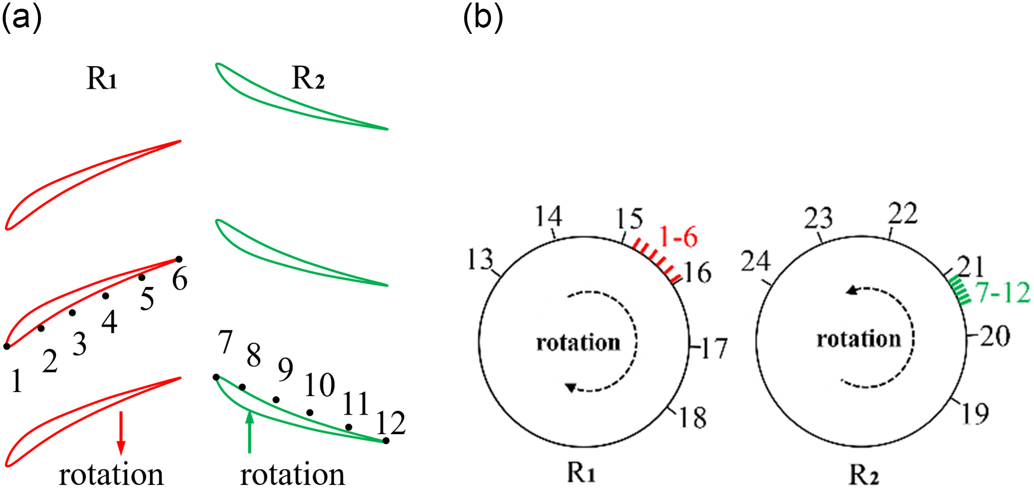
The contra-rotating compressor has a design speed of 3000 rpm of both rotors. The flow has apparent characteristics of rotating instability at 1800/2400rpm. Therefore, during the measurement, the rotating speed of the front and rear rotors is set at 1800 and 2400rpm, respectively. Twenty-four sensors are mounted in two layouts (i.e., chordwise and circumferential direction) with a sampling rate at 12.8kHz. All pressure sensors were installed with the sensor screen flush with the surface of the compressor casing for static pressure measurements. In the chordwise of both front rotor (R1) and the rear rotor (R2), six sensors are evenly arranged from the leading edge to the trailing edge, as can be seen in Fig. 2a. At the leading edge plane of the front rotor (R1), six sensors are evenly distributed along the circumferential direction in the range of 180 degrees. At 23.16% chord lengths upstream of the leading edge plane of the rear rotor (R2), six sensors are uniformly distributed in a 180-degree circumferential range in the circumferential direction. (Shown as Fig. 2b, the red and green bars represent the circumference position of sensors mounted in chordwise.)
Pressure sensors layout: (a) sensors along chordwise; (b) sensors along the circumferential direction.

3.0 METHODOLOGY
3.1 Double-phase-locking (DPL) technique
The flow in each blade passage in the compressor rotor is more or less different, so if the average flow condition must be observed over a while, a fixed blade passage must be specified. Because the blade passages rotate in real-time, and the pressure sensor installed at the top of the blade is immobile, it is necessary to find out the corresponding pressure value of the blade passage when it passes through the same sensor position twice adjacent to each other. These points are called in-phase points, and the process of obtaining in-phase points is called phase locking.
The phase-locking technique eliminates the disturbances fixed on the rotor, thereby highlighting the disturbances in the flow that is different from the blade passing frequency or rotor revolution frequency, and is therefore often used to characterise the average trajectory of the tip clearance flow. The phase-locking technique is widely used in the conventional layout (rotor-stator) axial flow compressors. In the contra-rotating compressor, because the front and rear rotors rotate in the opposite direction and the rotational speed is different, the traditional phase-locking technique cannot eliminate the interference of the front rotor wake to the rear rotor.
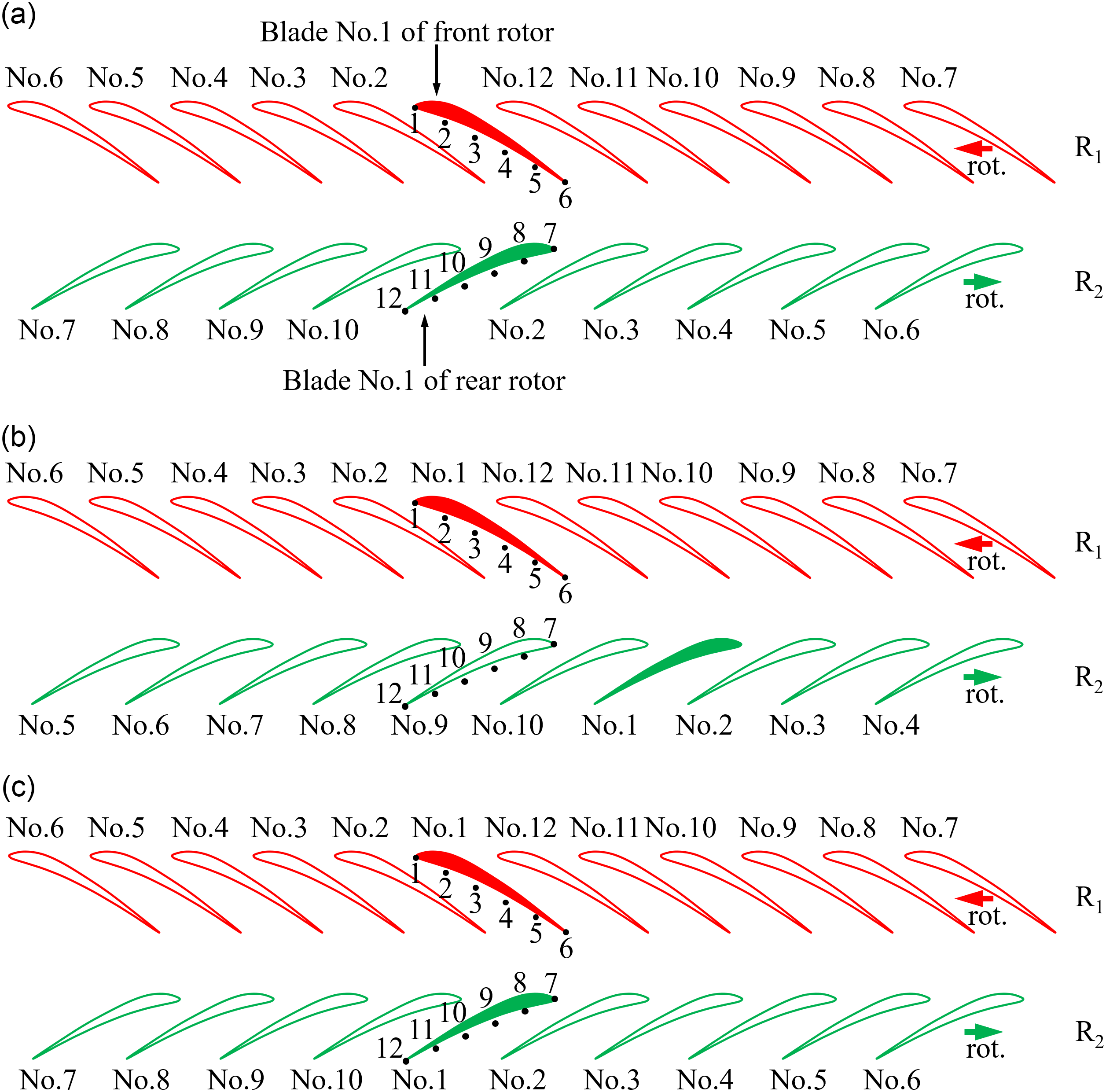
Principle of DPL: (a) t = 0; (b) t = i×T1, t $\,{\in}\,$j×T2(i, j
 $\,{\in}\,$N+); (c) t = i×T1 = j×T2(i, j
 $\in$N+).

This paper proposed a DPL technique designed for the contra-rotating compressor. The principle is shown in Fig. 3. The primary purpose of the method is to find the in-phase moments of the front and rear rotors. For the convenience of description, the front and rear rotor blades are numbered. Fig. 3a shows the initial spatial position of the No. 1 blade of the front and rear rotors. As time goes by, the No. 1 blade of the front rotor reaches its initial position, but the No. 1 blade of the rear rotor deviates from its initial position, so this moment is not the in-phase point of the front and rear rotors, as shown in Fig. 3b. Later, the No. 1 blade of both rotors simultaneously reaches their initial position, shown in Fig. 3c. Therefore, this moment is one in-phase point of the front and rear rotor. According to the DPL method, more in-phase points can be obtained, then the mean and root mean square (RMS) of the in-phase point sequence can be obtained to depict the average trajectory of the tip clearance flow in the contra-rotating compressor. The mean and RMS static pressure on blade tip casing under different flow conditions are ensemble-averaged over 60 cycles in this paper.
 \begin{equation}P_{\rm ens}=\frac{\sum\limits^{s-1}_{q=0}P(t+q\times T_{\rm dpl})}{s}\end{equation}
Where P ens is the local ensemble-averaged pressure, t is the current moment, q is integers, T dpl is the rotation period that obtained by DPL technique, s is positive integers.
 \begin{equation}P_{\rm rms}=\sqrt{\frac{\sum\limits^{s-1}_{q-0}[P(t+q\times T_{\rm dpl})-P_{\textrm{ens}}]^{2}}{s}}\end{equation}
Where P rms is the local root-mean-square pressure, t is the current moment, q is integers, Tdpl is the rotation period that obtained by DPL technique, P ens is the local ensemble-averaged pressure, and s is positive integers.
3.2 Normalised method
The normalisation process can make the pressure field of different flow conditions comparable. Therefore, this paper normalises the ensemble-averaged pressure to the  $\overline{P_{\textrm{ens}}}$. The specific formula is:
 \begin{equation}\overline{P}_{\rm ens}=(P_{\rm ens}-P_{\rm ens,min})/(P_{\rm ens,max}-P_{\rm ens,min})\end{equation}
where P ens is the local ensemble-averaged pressure, P min is the minimum value of the ensemble-averaged pressure field, P max is the maximum value of the ensemble-averaged pressure field.
Similarly, for the corresponding RMS result of the static pressure field, the normalised equation is:
 \begin{equation}\overline{P}_{\rm rms}=(P_{\rm rms}-P_{\rm rms,min})/(P_{\rm rms,max}-P_{\rm rms,min})\end{equation}
where P rms is the local value of the RMS pressure field, P rms,min is the minimum value of the RMS pressure field, P rms,max is the maximum value of the RMS pressure field.
3.3 Original modal estimation method
In general, mode decomposition for rotating instability requires a large number of monitoring sensors to be arranged along the circumference of the compressor. Such an experimental program can bring considerable time and economic costs. In fact, it is only necessary to arrange two sensors in the circumferential direction to calculate the mode number of rotating instability. The specific method is as follows: First, calculate the cross-spectrum of the pressure waves of the two sensors, and obtain the phase angle curve. Then, perform a least-square fit on the approximately linear portion of the phase angle curve to obtain a linear phase (represented by a straight line). Finally, calculate the average azimuthal phase velocity (AAPV) by the formula in equation (5), and obtain the mode number. See the appendix for the verification of this modal estimation method.
 \begin{equation}\mathrm{AAPV}=\Delta\theta/(\Delta\lambda/\Delta f)\end{equation}
Where Δ $\theta$ represents the circumferential angle difference of the two sensors, Δ
 $\lambda$ is the phase difference of the cross-spectrum, and Δf is the corresponding frequency difference in the cross-spectrum.
 \begin{equation}m_{\rm cal}=f_{\rm peak}/\mathrm{AAPV}\end{equation}
where m cal is the calculated mode number via the modal estimation method used in this paper, and f peak represents the frequency peak in coherence spectra.
 \begin{equation}Err=(m_{\rm cal}-m_{\rm real})/m_{\rm real}\times 100\%\end{equation}
where Err represents the relative error of the calculated mode number, and m real represents the real value of the mode number.
4.0 RESULTS
4.1 Overall performance
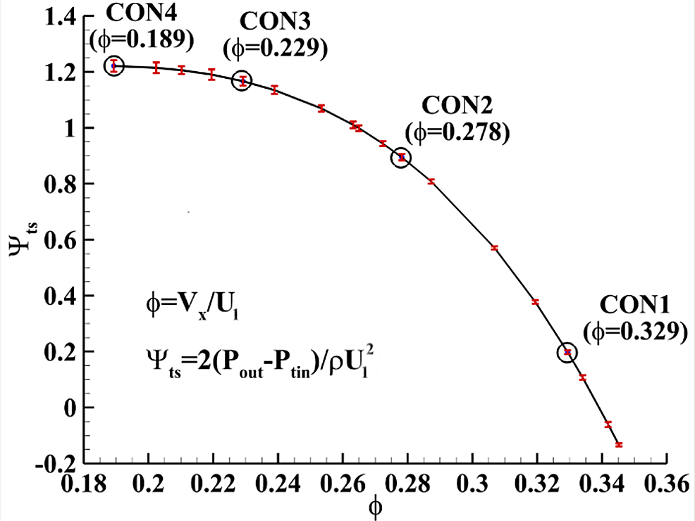
The total-to-static pressure coefficient curve (shown in Fig. 4) of the contra-rotating axial flow compressor is obtained by approaching the stall point using the method proposed in Ref. [Reference Mcdougall, Cumpsty and Hynes25]. Besides, the 95% confidence interval of each measurement point is marked with the red color error bars.
Total-to-static pressure ratio characteristics line (R1 = 1800rpm, R2 = 2400rpm).

4.2 Ensemble averaged static pressure contours using DPL technique at four flow conditions
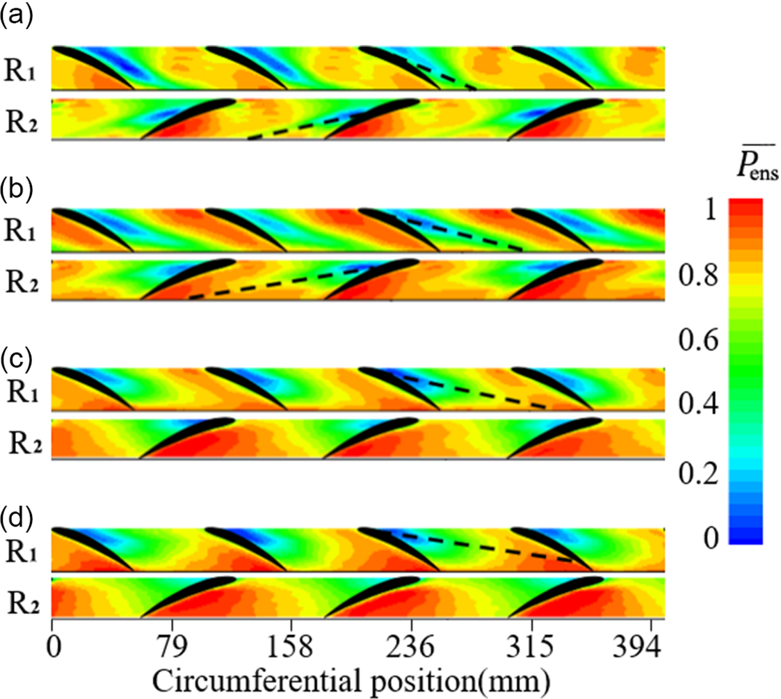
The averaged casing static pressure coefficient (normalised) of four different flow conditions is shown in Fig. 5. It can be seen that as the flow rate decreased (from CON1 to CON4), the low-pressure regions at the front and rear rotor blade passages gradually propagate upstream. In CON1, the low-pressure zone of the front rotor occupied the entire chordwise, and the low-pressure zone of the rear rotor is mainly concentrated in the middle of the blade. When the flow rate is reduced to CON2, the low-pressure region of the front rotor decreased along the chordwise, and the low-pressure zone of the rear rotor has moved forward to the vicinity of the blade leading edge plane. As the flow rate decreases to CON3, the low-pressure zone of the front rotor continues to move upstream, and the low-pressure zone of the rear rotor is still concentrated at the leading edge plane. When the flow rate decreases to CON4 (stall point), the low-pressure region of the front rotor continues to move upstream to the front half of the blade. The low-pressure region of the rear rotor has overflowed the leading edge plane. The low-pressure zone in the rotor blade tip represents the trajectory of the tip leakage vortex, so it can be found that the vortex core of both rotors moves upstream as the flow rate is reduced until the leading edge spillage occurred in the stall process.
Ensemble averaged static pressure contours on blade tip casing under different flow conditions. (The ensemble average over 60 cycles is applied, and the image is smoothed.) (a) CON1; (b) CON2; (c) CON3; (d) CON4.

4.3 RMS static pressure contours using DPL technique at four flow conditions
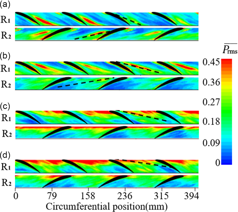
The RMS results of the rotor blade tip pressure at four different flow conditions are shown in Fig. 6. In CON1, a high RMS region is marked with black dotted lines in both rotors, which represents the trajectory of the tip leakage vortex. As the flow coefficient decreases to CON2, the angle between the trajectory of the tip leakage vortex of both rotors and the leading edge plane is reduced. When the flow rate continues to decrease to CON3, the trajectory of the tip leakage vortex of both rotors is already located in the leading edge plane. When the flow rate is reduced to CON4 (stall condition), the trajectory of the tip leakage vortex of the rear rotor is located upstream of the leading edge plane.
RMS static pressure contours on blade tip casing under different flow conditions. (This image uses the same original data as Fig. 5, and the image is smoothed.) (a) CON1; (b) CON2; (c) CON3; (d) CON4.

4.4 Fourier spectrum analysis
4.4.1 Rotating instability behavior at different flow conditions
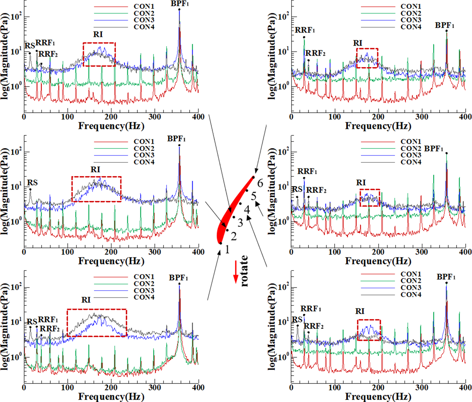
Fourier spectral analysis can depict the unsteady fluctuation characteristics of the tip clearance flow. The spectrum of the front rotor tip casing pressure at four different flow conditions is shown in Fig. 7. On the large flow conditions (CON1/CON2), there are mainly the rotor rotating frequency (RRF1) and its harmonics (for example, BPF1), and both show apparent peaks. At the same time, the rotation frequency of the R2 can also be found. Since the operating speed of R2 is higher than that of R1, its rotation frequency (RRF2) is also higher than the latter (RRF1). As the flow rate decreased to the small flow conditions (CON3/CON4), except for the intrinsic blade passing frequency (BPF1), there is broadband with no distinct peak and located around 0.5BPF1, which represents RI.
Fourier spectrum of the pressure wave of the front rotor tip.

Specifically, at flow rate CON3, the unstable fluctuation regions of the front and rear rotor tip clearance flow are located in the leading edge planes. The interference from rear rotor tip clearance flow on the front rotor is minimal, so the amplitude of the RI frequency band is gradually reduced from the leading edge to the trailing edge (sensor 1 to 6).
At flow rate CON4, the unsteady fluctuation region of the front rotor tip clearance flow is located in the leading edge plane, and the rear rotor tip clearance flow is located upstream of the leading edge. Therefore, the RI amplitude from the leading edge to the trailing edge is first decreased (sensors 1 to 4) and then increased (sensor 4 to 6) due to the unsteady fluctuation of the rear rotor tip clearance flow. Besides, rotating instability (RI) and the rotating stall (RS) both existed under this flow condition, and the amplitude of the stall disturbance decreased gradually from the leading edge to the trailing edge.
For the rear rotor, all sensors distributed along the chordwise did not capture the stall signal. Besides, some sensors have captured the characteristic frequency band of rotating instability. A reasonable explanation has not been given for this phenomenon. In order to ensure the integrity of the data presentation, the author puts the sensor pressure spectrum of the rear rotor in the appendix and will conduct more in-depth research on the results in the future.
4.4.2 Rotating instability behavior at different chordwise positions
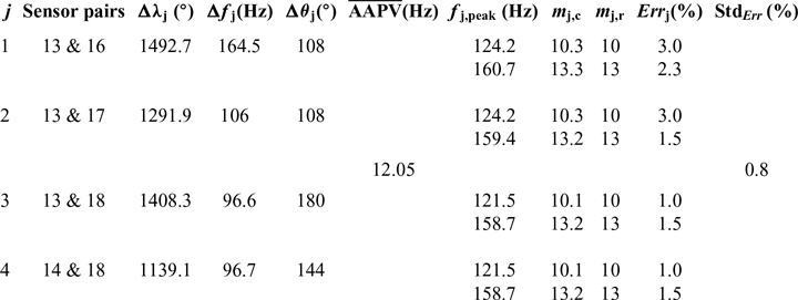
The unsteady characteristics of the tip clearance flow at four different chordwise positions in the front rotor are shown in Fig. 8. It can be found that under the flow coefficient CON3, the range of the RI band does not change with the chordwise position, and the amplitude is irregular from the leading edge to the trailing edge. When the flow coefficient dropped to CON4, the RI amplitude increased first (sensor 1 to 4) and then decreased (sensor 4 to 6). It should be noted that the original curve is resampled here. That is, some points are uniformly omitted so that the curve in the image is apparent without changing the trend of the original curve.
4.5 Improved modal estimation method
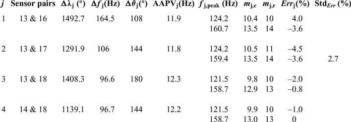
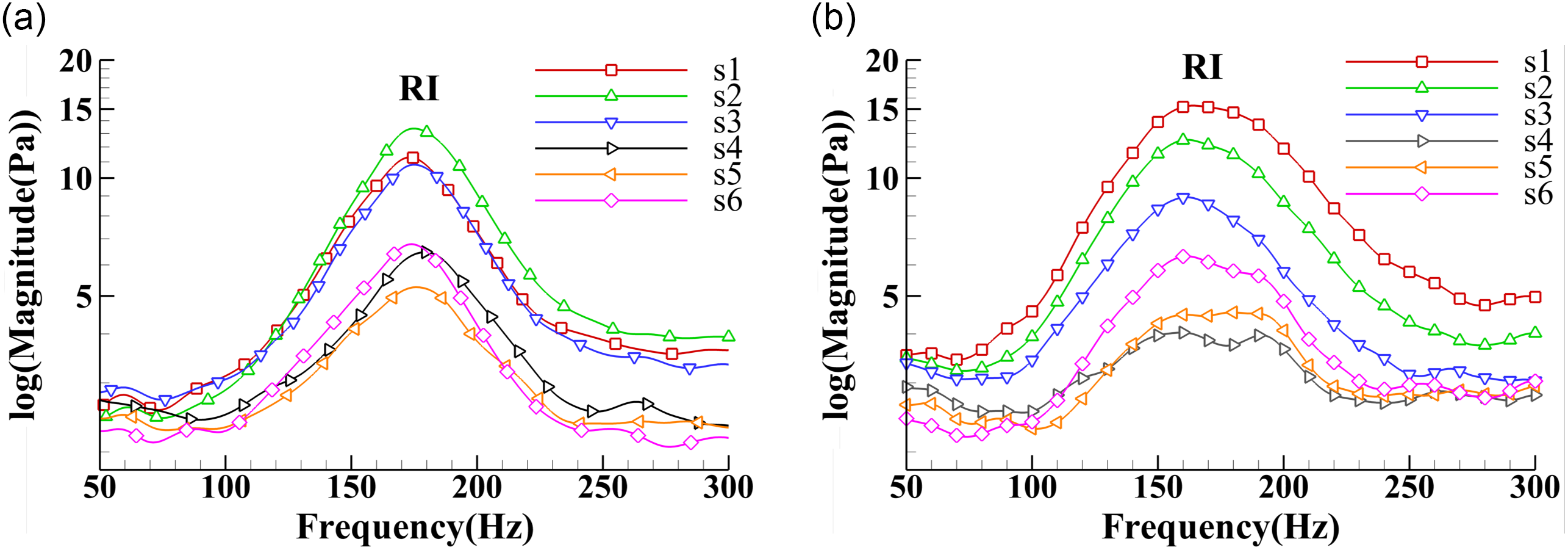
The mode number of rotating instability at CON4 is shown in Table 2 by using equation (8) to (13), with four pairs of sensor combinations involved in the calculation. The mode number directly calculated from the AAPV may not be an integer, therefore rounding up is necessary. Due to the subtle difference in the average angular azimuth phase velocities obtained by various sensor pairs, the mode numbers are different. Specifically, in the equation (9), the AAPV is located at the denominator, and the small fluctuation of the latter reflects the amplification effect on the former. The error caused by the rounding process may lead to the mode number to deviate from the truth. Therefore, the calculation error is reduced by correcting the AAPV. The detailed procedure is by calculating the mode number using the mean of the average azimuthal phase velocities of the four sensor pairs. In theory, sensors in the same circumferential plane should monitor the same average azimuth phase velocity, so this approach is reasonable. By using equation (14), results showed (Table 3) that the mode number rounding error is significantly reduced (from 2.7% to 0.8%), which makes the mode number more reliable.
Original modal estimation results of four sensor pairs (take the estimated results of modes 10 and 13 as an example)

Fourier spectrum of casing pressure waves of different chordwise positions: (a) CON3; (b) CON4.

Improved modal estimation results of four sensor pairs (take the estimated results of modes 10 and 13 as an example)

For easy understanding, an example of the estimation process of mode numbers 10 and 13 is given here.
Step 1: The circumferential angle difference Δ $\theta_{1}$ (108°) between the first sensor pairs (sensor 13 and 16) is obtained.
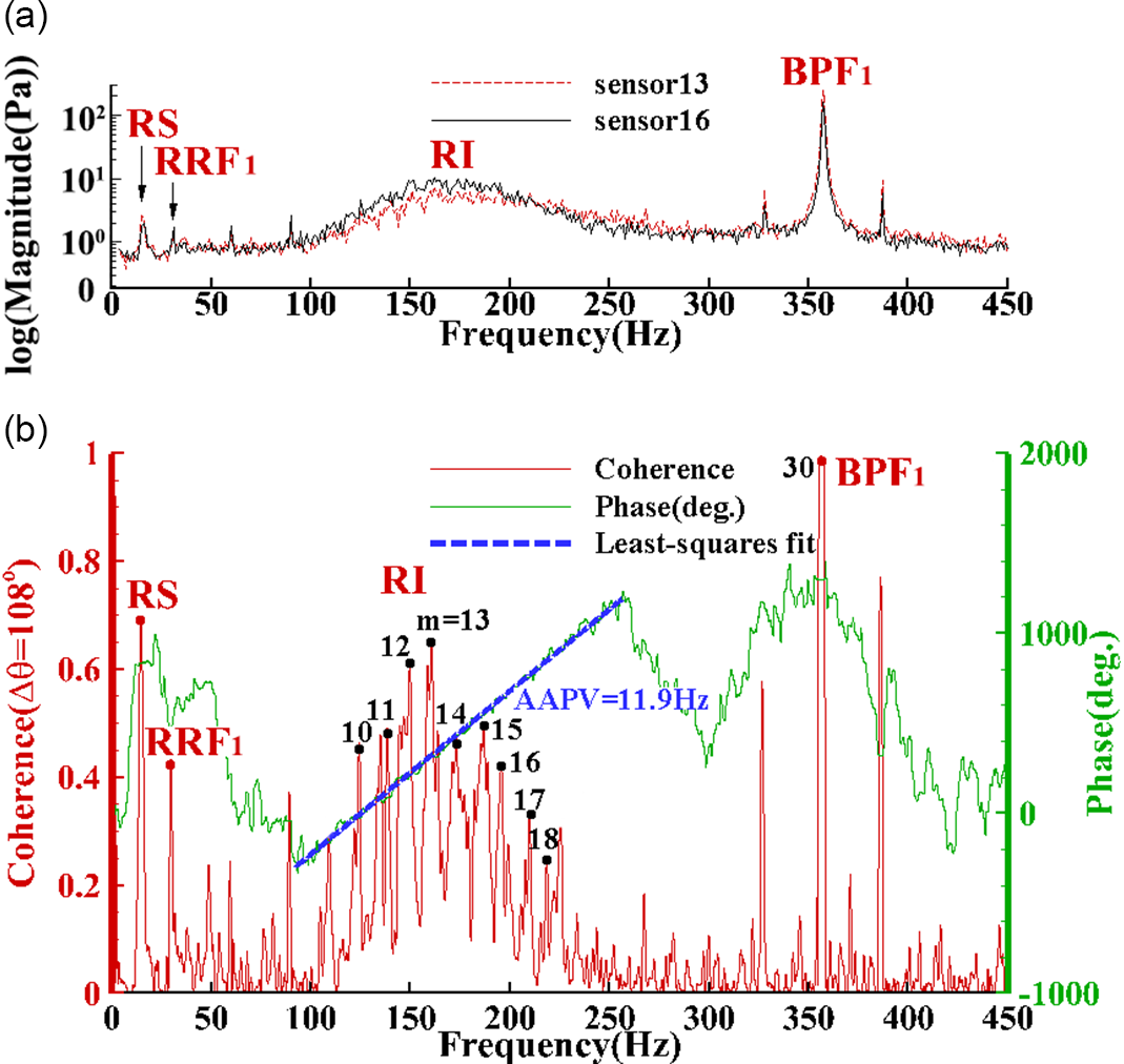
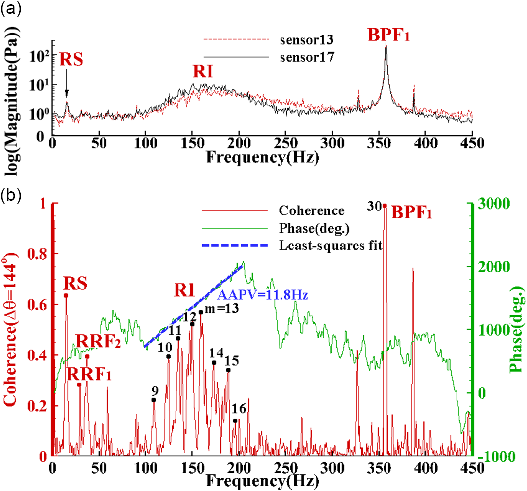
Step 2: The frequency spectrum of the pressure waves recorded by the two sensors is calculated, and it can be found that the approximate frequency range corresponding to the rotating instability is 100–260Hz, as shown in Fig. 9a.
Modal estimation (CON4: sensors 13 and 16).

Step 3: Calculating the cross-spectrum between the pressure waves was recorded by the two sensors and expand its phase, as shown by the green curve in Fig. 9b. There is an approximately linear part in the phase curve. By comparing with the frequency spectrum, it is found that the approximately linear part corresponds to the frequency band of rotating instability.
Step 4: Calculating the coherence spectrum between the pressure waves was recorded by the two sensors. As shown by the red curve in Fig. 9b, the coherence function exhibits multiple independent peaks at the position of the frequency band of rotating instability.
Step 5: The least-squares fitting is performed on the approximately linear part of the phase curve of cross-spectrum to obtain a line segment, as shown in the blue curve in Fig. 9b. The abscissa span of the line segment is Δf 1 (164.5Hz), the ordinate span is Δ $\lambda_{1}$ (1492.7°), and AAPV1 (11.9Hz) is calculated by Equation 8.
Step 6: Taking the two peak points f 1, peak (124.2Hz, and 160.7Hz, respectively) in the rotating instability frequency band in the coherence spectrum as examples, the mode numbers m 1,c of the two peak points are calculated by Equation 9 (10.4 and 13.5, respectively).
Step 7: Round the mode numbers calculated above to obtain the corresponding rounded modal numbers m 1,r (10 and 14, respectively), as shown in Equation 10.
Step 8: The relative error Err 1 of m 1,c is calculated by Equation 11, which is 4.0% and 6%, respectively.
Step 9: Steps 1 to 8 are implemented for the second to fourth sensor pairs, respectively, to obtain Err 2 to Err 4.
Step 10: Calculate the standard deviation Std Err (2.7%) of relative error through Equations 12 and 13, and then all the data in Table 2 can be obtained.
Step 11: The arithmetic average of AAPVj corresponding to the four sensor pairs is obtained by Equation 14, namely  $\overline{\mathrm{AAPV}}$ (12.05Hz).
Step 12: Replace AAPVj with  $\overline{\mathrm{AAPV}}$ and repeat Steps 6 to 10 to get all the data in Table 3.
Refer to(Reference Liu, Holste and Neise8) for the calculation method of cross-spectrum and its phase.
 \begin{equation}\mathrm{AAPV}_{\rm j}=\Delta\theta_{\rm j}/(\Delta\lambda_{\rm j}/\Delta f_{\rm j})\end{equation}
where Δ $\theta$j represents the circumferential angle difference of the jth sensor pair, Δ
 $\lambda$j is the phase difference of the cross-spectrum, and Δf is the corresponding frequency difference in the cross-spectrum.
 \begin{equation}m_{\rm j,c}=f_{\rm j,peak}/\mathrm{AAPV}_{\rm j}\end{equation}
where m j,c is the calculated mode number via the modal estimation method used in this paper, and f j,peak represents the frequency peak in coherence spectra.
 \begin{equation}m_{\rm j,x}=round(m_{\rm j,c})\end{equation}
where m j,r represents the corrected mode number, and m j,c represents the directly calculated mode number.
 \begin{equation}Err_{\rm j}=(m_{\rm j,c}-m_{\rm j,r})/m_{\rm j,r}\times 100\%\end{equation}
where Err represents the relative error of the calculated mode number, and m real represents the real value of the mode number.
Modal estimation (CON4: sensors 13 and 17).

 \begin{equation}Err_{\rm mean}=\frac{1}{n}\sum^{n}_{j=1}Err_{\rm j}\end{equation}
where E mean represents the arithmetic mean of the corresponding E j for different sensor pairs, j is the index of the sensor pair, and n is the total number of sensor pairs.
 \begin{equation}Std_{\rm Err}=\sqrt{\frac{1}{n}\sum^{n}_{j=1}(Err_{\rm j}-Err_{\rm mean})}\end{equation}
where Std Err represents the standard deviation of the corresponding Err j for different sensor pairs, j is the index of the sensor pair, and n is the total number of sensor pairs.
 \begin{equation}\overline{\textrm{AAPV}}=\frac{1}{n}\sum^{n}_{j=1}(\mathrm{AAPV}_{\rm j})\end{equation}
where  $\overline{\mathrm{AAPV}}$ represents the arithmetic mean of the corresponding AAPV for different sensor pairs, j is the index of the sensor pair, and n is the total number of sensor pairs.
Modal estimation (CON4: sensors 13 and 18).

Modal estimation (CON4: sensors 14 and 18).

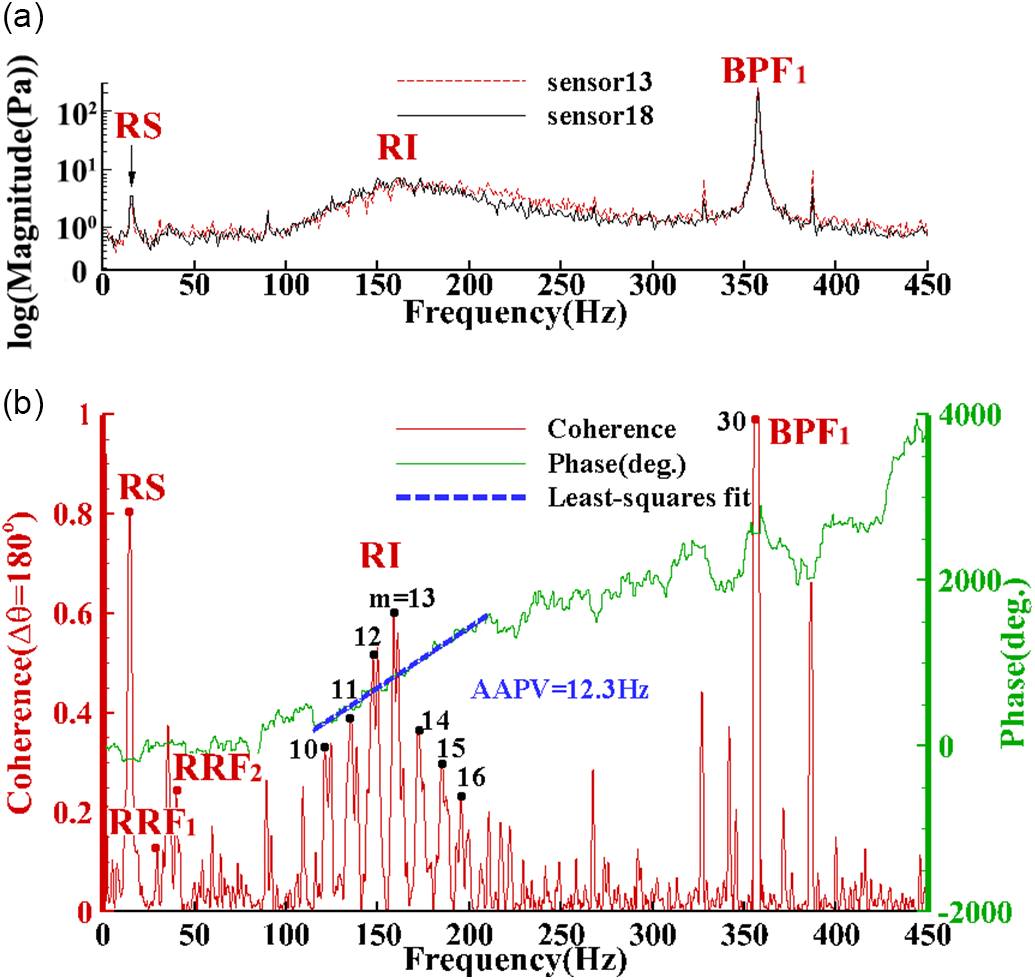
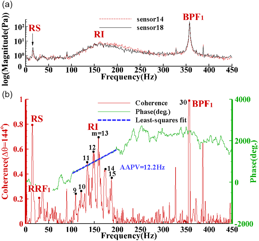
The improved modal estimation results of rotating instability at CON4 is shown as Figs. 9–12, where the upper half plot (that is, a, and SPL represents the sound pressure level) in each figure is the frequency spectrum of the two circumferentially distributed sensors. The lower half (that is, b) is the coherence and cross-spectrum phase angle. The rotating instability frequency band locates in the range of 100 to 250Hz, and the rotating stall (RS) frequency is around 14.5Hz. The rotating stall frequency is about half of the shaft frequency (or rotor rotating frequency, RRF1), and the RI frequency band (centered in 175Hz) is nearly half of the blade passing frequency (BPF1). It can be found that each peak of the rotating instability frequency band corresponds to a unique dominant circumferential mode and the mode number 13 has the highest amplitude. Besides, the frequency interval between adjacent modes equals to the AAPV (shown in Table 2). This modal estimation method is only applicable to the calculations within the rotating instability frequency band. There may be some deviations in the calculation results at the boundary points of the frequency band.
5.0 CONCLUSION
Rotating instability is a kind of flow disturbance that is different from the rotating stall. The most significant difference between it and the rotating stall in the frequency spectrum is that the former exhibits multi-peak broadband characteristics, and the latter exhibits single-peak characteristics. To explore the reasons for this difference, the mode decomposition method has become the primary means to explain this phenomenon. While the traditional modal decomposition method requires a large number of sensors, the improved modal estimation method proposed in this paper can achieve reliable modal number estimation with a small number of sensors. In this paper, the rotating instability in a low-speed axial flow contra-rotating compressor is studied. The following conclusions are obtained by installing the high-frequency response pressure sensor sparse array on the casing wall in the circumferential direction and chordwise:
1) A DPL technique suitable for the contra-rotating compressor is proposed. By using this method, it is shown that the trajectory of the tip leakage vortex in the rear rotor is located upstream of the leading edge plane at the stall condition.
2) The Fourier spectrum indicates that the stall and the rotating instability both occurred in the compressor, and the frequency band of rotating instability does not change with the flow rate.
3) By optimising the AAPV, a compact modal estimation method is obtained to solve the mode number. This method dramatically reduces the experimental cost and has a wide range of engineering application values.
ACKNOWLEDGEMENTS
This work has been supported by the National Natural Science Foundation of China (No. 51376150, No. 51906205) and National Science and Technology Major Project (2017-II-0009-0023).
APPENDIX
The modal estimation method was validated repeatedly with the data adopted from Ref. [Reference Pardowitz, Tapken and Enghardt20]. The verification results showed that this method achieved the goal; that is, it is useful to solve the mode number by using AAPV.
Modal estimation method verification detail with data adopted from Ref. [Reference Pardowitz, Tapken and Enghardt20]

shows the modal estimation method validation with data adopted from Ref. [Reference Pardowitz, Tapken and Enghardt20]: (a) phase angle of cross-spectrum; and (b) circumferential modes amplitudes.

shows the Fourier spectrum of the pressure wave of the rear rotor tip Figure A2 (a)-(f) represents sensors 7 to 12.

As showed in Table A1 and Fig. A1a, Δf = 217Hz, Δ $\lambda=360$°, and Δ
 $\theta=77$° in the Ref. Reference Pardowitz, Tapken and Enghardt20 so that the following modal estimation results can be calculated according to the equation (5) to (7).
Figure A2 shows the Fourier spectrum results of the pressure signal monitored by the sensor installed along the chordwise on the tip of the rear rotor. Figure A2 (a)-(f) corresponds to sensors 7 to 12; that is, from the leading edge to the trailing edge of the rear rotor. For the specific positions of the sensors, refer to Fig. 2a. Sensor 7 and sensor 8 did not detect the characteristic frequency band corresponding to the rotating instability phenomenon. Starting from sensor 9, the rotating instability frequency band begins to appear and becomes more and more evident as the position approaches the trailing edge. This phenomenon is different from the front rotor. It needs further in-depth research in the future to give a reasonable explanation. The corresponding frequency of the stall cell propagating in the circumferential direction was not monitored in the chord direction of the rear rotor.