1 Introduction
Two-phase gas–liquid turbulent flows where phase change takes place are relevant to many natural processes such as rain formation and numerous industrial applications, such as heat exchangers, boilers and combustion engines. An internal combustion engine is a complex energy conversion system, where the fuel spray interacts with its surrounding gas exchanging momentum, heat and mass. The breakup of a spray implies the formation of smaller structures as liquid sheets, ligaments and droplets. For an atomization breakup regime, where the flow is turbulent with high Reynolds number, droplet sizes much smaller than the initial spray diameter are observed (Lefebvre Reference Lefebvre1989).
Theoretical modelling of drop breakup mechanisms and different aspects of drop deformation have been covered over the years (Lasheras et al.
Reference Lasheras, Eastwood, Martínez-Bazán and Montañés2002). The breakup prediction of a droplet in a turbulent flow was first proposed by Hinze (Reference Hinze1955) and was based on establishing a critical Weber number according to different flow conditions. For the condition of this critical number being exceeded, surface tension would be unable to balance inertia forces and the droplet would break. In isotropic turbulence, the maximum critical stable droplet diameter
 $D_{max}$
defined by Hinze is given as
 $$\begin{eqnarray}D_{max}=C\left(\frac{\unicode[STIX]{x1D70E}}{\unicode[STIX]{x1D70C}_{v}}\right)^{3/5}\unicode[STIX]{x1D700}^{-2/5},\end{eqnarray}$$
where
 $\unicode[STIX]{x1D70E}$
denotes the surface tension,
 $\unicode[STIX]{x1D70C}_{v}$
the vapour density and
 $\unicode[STIX]{x1D700}$
the turbulent energy dissipation rate. The coefficient
 $C$
is obtained by fitting experimental data. In other words, Hinze showed that a droplet is stable if
 $D<D_{max}$
or that it would deform and break if
 $D>D_{max}$
, due random pressure fluctuations generated from turbulence. The prediction by Hinze has also been used and compared for breakup of bubbles, both experimentally (Walter & Blanch Reference Walter and Blanch1986; Risso & Fabre Reference Risso and Fabre1998) and numerically (Qian et al.
Reference Qian, McLaughlin, Sankaranarayanan, Sundaresan and Kontomaris2006). Perlekar et al. (Reference Perlekar, Biferale, Sbragaglia, Srivstava and Toschi2012) studied the breakup of droplet in the context of emulsions. By using a lattice Boltzmann method (LBM) with a fluid–fluid interface, the effects of turbulent fluctuations and surface tension on the droplet disruption were investigated. Perlekar et al. (Reference Perlekar, Biferale, Sbragaglia, Srivstava and Toschi2012) performed droplet size distribution analyses with identical density and viscosity for the droplet and surrounding fluid. They observed that breakup events are associated with peaks in the local energy dissipation rate in the droplet neighbourhood. A similar LBM approach was used by Skartlien, Sollum & Schumann (Reference Skartlien, Sollum and Schumann2013), where the presence of surfactants in emulsions with moderate viscosity ratio was taken into account. Due to the decrease of surface tension and presence of Marangoni effects, the breakup scale does not follow Hinze’s inviscid prediction.
The understanding of droplet deformation is important even when breakup does not take place. Having in mind rheological properties of suspensions and the behaviour of red blood cells, Biferale, Meneveau & Verzicco (Reference Biferale, Meneveau and Verzicco2014) studied small ellipsoidal droplets with unity viscosity ratio, exploring the coupling between droplet deformation and orientation. They also examined variations of the ratio of droplet to carrier fluid viscosities, with discussions on difficulties in simulating different viscosities. Scarbolo & Soldati (Reference Scarbolo and Soldati2013) analysed the interaction between turbulence and surface tension for a non-breaking large deformable droplet. They have considered an emulsion with same viscosity and density in a wall-bounded turbulence, focusing on the turbulent field at the droplet surface. A damping of the turbulence intensity near the interface is observed, with a vorticity generation that is dependent on the surface tension. These effects are also seen at larger distances from the interface by increasing surface tension. Scarbolo & Soldati (Reference Scarbolo and Soldati2015) used the same approach to further investigate the effects of deformation of many large droplets in a turbulent channel flow. The wall drag is seen to increase by less deformability, which is due to the change in the slip velocity of the droplets.
However, a key point to connect the investigation of deformable droplets in turbulent flows with energy conversion systems is lacking: the heat and mass transfer between the different fluid phases has not been carefully investigated. In the presence of turbulence, coherent structures with strong shear layers may affect the mass and heat transfer between the liquid–vapour flows, which may result in modifying the degree of droplet deformation. The droplet dynamics considered in these circumstances would shed more light on how to better optimize and understand energy conversion systems.
The main issue in performing simulations in this context remains in the challenging description of interfacial mass, momentum and energy conservation coupled to surface tension and latent heat effects. Lately, the LBM with phase change has proven to be a suitable numerical method for treating multiphase flows (Li et al. Reference Li, Luo, Kang, He, Chen and Liu2016). The mesoscopic nature of LBM includes only a minimal amount of microscopic details in order to reproduce interfacial physics and macroscopic flow hydrodynamics in a consistent manner (Safari, Rahimian & Krafczyk Reference Safari, Rahimian and Krafczyk2013, Reference Safari, Rahimian and Krafczyk2014). The LBM thus avoids the need of tracking the interface due to its diffusive interface approach. An advantage of this method is that the computational work is independent of the number of droplets/bubbles. However, multiphase LBM has been criticized due to large spurious currents produced near curved interfaces (Sbragaglia et al. Reference Sbragaglia, Benzi, Biferale, Succi, Sugiyama and Toschi2007), especially when a large density ratio is considered. The resulting instability from these currents can restrict what parameters may be simulated, e.g. when performing simulations with turbulent flows. Many studies have been focused on improvements of multiphase LBM, resulting in a numerically stable model with significant reduction of spurious currents (Connington & Lee Reference Connington and Lee2012). Furthermore, LBM also presents a convenient framework to incorporate thermodynamic effects, which naturally generates the phase separation.
In the present study we examine the dynamics of a droplet surrounded by its own vapour in isotropic turbulence. The heat and mass transfer are taken into consideration as well as density and viscosity contrast between the two phases. We are interested in simulating a large droplet, which is much larger than the Kolmogorov length. Results herein are presented for droplet radius between 25 and 40 times larger than the Kolmogorov length scale. The treatment for such a case is completely different than the one used for droplets of the order of the Kolmogorov length, where point particles approximation can be used (Toschi & Bodenschatz Reference Thomson2009). A LBM that allows the inclusion of a non-ideal equation of state (EOS) is used for solving the momentum equations, whereas the energy equation is solved by a finite difference scheme. The phase change has been covered and validated in previous publications by the authors (Albernaz, Do-Quang & Amberg Reference Albernaz, Do-Quang and Amberg2015; Albernaz, Amberg & Do-Quang Reference Albernaz, Amberg and Do-Quang2016a ). Isotropic turbulence is commonly used by direct numerical simulations and is based on the addition of a forcing term that generates fluctuations in hydrodynamic variables in time and space for different scales (Ishihara, Gotoh & Kaneda Reference Ishihara, Gotoh and Kaneda2009). Thermodynamic variables have recently been investigated by Albernaz, Do-Quang & Hermanson (Reference Albernaz, Do-Quang, Hermanson and Amberg2016b ) for a single phase in isotropic turbulence approaching critical conditions. Here, we are interested in the coupling between the droplet deformation, the phase change between liquid–vapour, the turbulence fluctuations and changes in thermodynamic variables.
The paper is organized as follows. In § 2 the numerical method is presented and validated with a careful discussion on how the equilibrium condition is controlled so that a stationary state is reached and statistics can be performed. In § 3 we simulate a droplet under the same Taylor Reynolds number, where the focus is to quantify and analyse the effects of changing the Ohnesorge number by either changing the surface tension or the droplet size. Fluctuations and variance of thermodynamic variables are also taken into consideration. In § 4 we examine how the Taylor Reynolds number affects the turbulent quantities and the energy spectra. These changes are also related to the droplet deformation and Weber number. The oscillation frequency of the droplet is shown in § 5, where the temporal spectra of the deformation parameter are discussed. Correlation coefficients are also introduced in order to give strong support to our analyses along with joint probability distribution functions between different variables. The conclusions are presented in § 6.
2 Numerical method
In order to solve the momentum equations, a three-dimensional nineteen-velocity (D3Q19) pseudopotential LBM is considered. The evolution equation of the density distribution function is given by
 $$\begin{eqnarray}f_{i}(\boldsymbol{x}+\boldsymbol{c}_{i}\unicode[STIX]{x1D6FF}_{t},t+\unicode[STIX]{x1D6FF}_{t})=f_{i}(\boldsymbol{x},t)+\unicode[STIX]{x1D6FF}_{t}\unicode[STIX]{x1D6EC}_{i}+\unicode[STIX]{x1D6FF}_{t}F_{i}^{\prime }+3\unicode[STIX]{x1D6FF}_{t}\unicode[STIX]{x1D70C}\unicode[STIX]{x1D714}_{i}[\boldsymbol{c}_{i}\boldsymbol{\cdot }\boldsymbol{F}_{T}],\end{eqnarray}$$
where
 $f_{i}$
is the density distribution function,
 $t$
is time and
 $\unicode[STIX]{x1D6FF}_{t}$
is the time step. The notation
 $i$
is given as
 $i=0,\ldots ,N$
, where
 $N$
denotes the number of directions of the particle velocities at each node. The lattice velocity is given by
 $\boldsymbol{c}_{i}$
and
 $\boldsymbol{x}$
is the spatial position. The coefficients
 $\unicode[STIX]{x1D714}_{i}$
for the D3Q19 lattice are given as
 $\unicode[STIX]{x1D714}_{0}=1/3$
,
 $\unicode[STIX]{x1D714}_{1{-}6}=1/18$
and
 $\unicode[STIX]{x1D714}_{7{-}18}=1/36$
. The force
 $F_{i}^{\prime }$
is the interaction force that takes molecular interactions in consideration, while
 $\boldsymbol{F}_{T}$
denotes the turbulent forcing applied to the flow field. The change of
 $f_{i}$
due to collisions is represented by
 $\unicode[STIX]{x1D6EC}_{i}$
. The multirelaxation time (MRT) collision operator (Lallemand & Luo Reference Lallemand and Luo2000) is used to ensure numerical stability. Details about the MRT model can be found in d’Humieres et al. (Reference d’Humieres, Ginzburg, Krafczyk, Lallemand and Luo2002). The pseudopotential force is incorporated into LBM by using the exact difference method (EDM) by Kupershtokh & Medvedev (Reference Kupershtokh and Medvedev2006), which can be written as
 $$\begin{eqnarray}F_{i}^{\prime }=\unicode[STIX]{x1D714}_{i}\left[\frac{\boldsymbol{c}_{i}\boldsymbol{\cdot }\boldsymbol{F}^{\prime }}{c_{s}^{2}}+\frac{(\boldsymbol{c}_{i}\boldsymbol{\cdot }\boldsymbol{u})(\boldsymbol{c}_{i}\boldsymbol{\cdot }\boldsymbol{F}^{\prime })}{c_{s}^{4}}-\frac{\boldsymbol{u}\boldsymbol{\cdot }\boldsymbol{F}^{\prime }}{c_{s}^{2}}\right],\end{eqnarray}$$
where
 $\boldsymbol{F}^{\prime }$
is the interparticle interaction force, which accounts for mesoscopic forces acting between neighbour nodes. The lattice Boltzmann speed of sound is given by
 $c_{s}=1/\sqrt{3}\unicode[STIX]{x1D6FF}_{x}/\unicode[STIX]{x1D6FF}_{t}$
,
 $\unicode[STIX]{x1D6FF}_{x}$
being the lattice space unit. The density
 $\unicode[STIX]{x1D70C}$
and actual fluid velocity
 $\boldsymbol{u}$
are calculated by
 $$\begin{eqnarray}\unicode[STIX]{x1D70C}=\mathop{\sum }_{i}f_{i},\quad \boldsymbol{u}=\boldsymbol{u}^{eq}+\frac{\boldsymbol{F}^{\prime }}{2\unicode[STIX]{x1D70C}},\end{eqnarray}$$
where the equilibrium velocity assumes
 $\boldsymbol{u}^{eq}=1/\unicode[STIX]{x1D70C}\sum _{i}\boldsymbol{c}_{i}f_{i}$
(details can be found in Li, Luo & Li Reference Li, Luo and Li2012). The local force is based on a linear combination of the local and the mean value gradient approximations as proposed by Kupershtokh, Medvedev & Karpov (Reference Kupershtokh, Medvedev and Karpov2009), given by
 $$\begin{eqnarray}\displaystyle \boldsymbol{F}^{\prime }=\frac{A}{c_{s}^{2}}\mathop{\sum }_{i=1}^{18}\unicode[STIX]{x1D714}_{i}\unicode[STIX]{x1D6F7}^{2}(\boldsymbol{x}+\boldsymbol{c}_{i})\boldsymbol{c}_{i}+\frac{(1-2A)}{c_{s}^{2}}\unicode[STIX]{x1D6F7}(\boldsymbol{x})\mathop{\sum }_{i=1}^{18}\unicode[STIX]{x1D714}_{i}\unicode[STIX]{x1D6F7}(\boldsymbol{x}+\boldsymbol{c}_{i})\boldsymbol{c}_{i}, & & \displaystyle\end{eqnarray}$$
where
 $A$
is a correlative fitting parameter. The special function
 $\unicode[STIX]{x1D6F7}$
is given by
 $\unicode[STIX]{x1D6F7}=\sqrt{\unicode[STIX]{x1D70C}c_{s}^{2}-\unicode[STIX]{x1D705}p}$
, where
 $\unicode[STIX]{x1D705}$
sets the thickness of the interface when both liquid and vapour coexist. The surface tension value is also changed by
 $\unicode[STIX]{x1D705}$
. The droplet interface is seen to consist of 4–8 lattice points for the different values of
 $\unicode[STIX]{x1D705}$
chosen in the present work. Pressure is related to density and temperature by the inclusion of a non-ideal EOS, which is responsible for controlling the phase change between liquid–vapour. We choose the Peng–Robinson (PR) EOS which has shown as a suitable EOS to represent hydrocarbon fluids close to the critical point (Balaji et al.
Reference Balaji, Ramamurthi and Gogos2011). The PR EOS is written as
 $$\begin{eqnarray}p=\frac{\unicode[STIX]{x1D70C}RT}{1-b\unicode[STIX]{x1D70C}}-\frac{a\unicode[STIX]{x1D70C}^{2}\unicode[STIX]{x1D6FC}^{\prime }(T)}{1+2b\unicode[STIX]{x1D70C}-b^{2}\unicode[STIX]{x1D70C}^{2}},\end{eqnarray}$$
where
 $a=0.45724R^{2}T_{c}^{2}/p_{c}$
and
 $b=0.0778RT_{c}/p_{c}$
. The subscript
 $c$
denotes the evaluation at the critical point. The parameter
 $\unicode[STIX]{x1D6FC}^{\prime }(T)=[1+(0.37464+1.54226w-0.26992w^{2})(1-\sqrt{T/T_{c}})]^{2}$
is defined according to the acentric factor
 $w$
and the actual temperature
 $T$
. A hexane fluid is taken into consideration, with
 $w=0.30075$
. For the PR EOS, a value of
 $A=-0.07$
has been shown to yield an accurate reproduction of the coexistence curves for hexane fluid (Albernaz et al.
Reference Albernaz, Do-Quang and Amberg2015). Through a Chapman–Enskog (C–E) analysis, the mass and momentum conservation equations are obtained at the macroscopic scale, given respectively as
 $$\begin{eqnarray}\displaystyle & \displaystyle \frac{\unicode[STIX]{x2202}\unicode[STIX]{x1D70C}}{\unicode[STIX]{x2202}t}+\unicode[STIX]{x1D735}\boldsymbol{\cdot }(\unicode[STIX]{x1D70C}\boldsymbol{u})=0, & \displaystyle\end{eqnarray}$$
 $$\begin{eqnarray}\displaystyle & \displaystyle \frac{\unicode[STIX]{x2202}}{\unicode[STIX]{x2202}t}(\unicode[STIX]{x1D70C}\boldsymbol{u})+\unicode[STIX]{x1D735}\boldsymbol{\cdot }(\unicode[STIX]{x1D70C}\boldsymbol{u}\boldsymbol{u})=-\unicode[STIX]{x1D735}p+\unicode[STIX]{x1D735}\boldsymbol{\cdot }(2\unicode[STIX]{x1D707}\boldsymbol{S})+\boldsymbol{F}^{\prime }+\boldsymbol{F}_{T}, & \displaystyle\end{eqnarray}$$
where
 $\unicode[STIX]{x1D707}$
is the dynamic viscosity and
 $\boldsymbol{S}=(\unicode[STIX]{x1D735}\boldsymbol{u}+(\unicode[STIX]{x1D735}\boldsymbol{u})^{\text{T}})/2$
the deviatoric stress. The dynamic viscosity is given as a function of the relaxation time
 $\unicode[STIX]{x1D70F}_{\unicode[STIX]{x1D708}}$
, being
 $\unicode[STIX]{x1D707}=\unicode[STIX]{x1D70C}c_{s}^{2}(\unicode[STIX]{x1D70F}_{\unicode[STIX]{x1D708}}-1/2)$
. We make use of a solenoidal forcing for a lattice Boltzmann method proposed by Kareem et al. (Reference Kareem, Izawa, Xiong and Fukunishi2009), which is applied every time step to generate a statistical stationary velocity field. The three components of the forcing
 $\boldsymbol{F}_{T}=(F_{T,x},F_{T,y},F_{T,z})$
are defined as
 $$\begin{eqnarray}\displaystyle \left.\begin{array}{@{}c@{}}F_{T,x}=2a\left({\displaystyle \frac{k_{y}k_{z}}{k^{2}}}\right)G(k_{x},k_{y},k_{z})\\ F_{T,y}=-a\left({\displaystyle \frac{k_{x}k_{z}}{k^{2}}}\right)G(k_{x},k_{y},k_{z})\\ F_{T,z}=-a\left({\displaystyle \frac{k_{x}k_{y}}{k^{2}}}\right)G(k_{x},k_{y},k_{z}),\end{array}\right\} & & \displaystyle\end{eqnarray}$$
here
 $G(k_{x},k_{y},k_{z})$
is given by
 $$\begin{eqnarray}G(k_{x},k_{y},k_{z})=\sin \left[\frac{2\unicode[STIX]{x03C0}x}{L}k_{x}+\frac{2\unicode[STIX]{x03C0}y}{L}k_{y}+\frac{2\unicode[STIX]{x03C0}z}{L}k_{z}+\unicode[STIX]{x1D711}\right],\end{eqnarray}$$
where
 $L$
denotes the dimensionless length of the domain (based on the lattice space unit
 $\unicode[STIX]{x1D6FF}_{x}$
) and
 $\unicode[STIX]{x1D711}$
is the random phase, which is updated every 10 time steps. Please note that
 $L$
is a non-dimensional quantity based on the reference lattice space unit
 $\unicode[STIX]{x1D6FF}_{x}$
. It is important to mention that the density which multiplies the turbulent force in (2.1) is taken as the vapour density. This way, the turbulent forcing is homogeneous throughout the domain, where both phases experience the same forcing magnitude. Since the droplet is heavier than the surrounding vapour, it is expected that the vapour moves faster than the droplet. Additionally, one should note that both phases present the same kinetic energy, where the density ratio scales with velocity ratio
 $\unicode[STIX]{x1D70C}_{\ell }/\unicode[STIX]{x1D70C}_{v}\sim u_{v}^{2}/u_{\ell }^{2}$
, where
 $\ell$
denotes liquid and
 $v$
the vapour phase.
The forcing amplitude
 $a$
controls the turbulence intensity and therefore the Taylor Reynolds number, given as
 $Re_{\unicode[STIX]{x1D706}}=\unicode[STIX]{x1D706}\sqrt{2E/3}/\unicode[STIX]{x1D708}$
, with
 $\unicode[STIX]{x1D708}$
being the kinematic viscosity. The kinetic energy is given as
 $E=(\sum _{\boldsymbol{x}}u^{2})/L^{3}$
and
 $\unicode[STIX]{x1D706}=\sqrt{15E\unicode[STIX]{x1D708}/\unicode[STIX]{x1D700}}$
is the Taylor microscale. The term
 $\unicode[STIX]{x1D700}=\unicode[STIX]{x1D708}\sum _{\boldsymbol{x}}(\unicode[STIX]{x1D735}u)^{2}/L^{3}$
corresponds to the energy dissipation rate per unit volume. The three-dimensional wavenumber is given by
 $(k_{x},k_{y},k_{z})$
. It is important to mention that the forcing takes place only for low wavenumber, i.e.
 $k\leqslant 3$
.
There are many methods to simulate thermal effects. The thermal lattice Boltzmann method can be used (McNamara Reference McNamara1995), where the macroscopic energy equation needs to be explicitly corrected due to the presence of deviation terms (Márkus & Házi Reference Márkus and Házi2011). One could treat this issue by using a MRT modelling and modifying the relaxation matrix and equilibrium distribution function (Huang & Wu Reference Huang and Wu2014). Another approach is by applying a hybrid method, where the energy equation is solved by finite-difference (FD) scheme (Lallemand & Luo Reference Lallemand and Luo2003b
; Treeck et al.
Reference Treeck, Rank, Krafczyk, Toelke and Nachtwey2006) and is employed in the present study. Due to the absence of correction terms, numerical errors are reduced. The equation of energy can be given in terms of the fluid temperature
 $T$
. For a Newtonian fluid with varying thermal conductivity
 $k$
, the energy equation is given as (Bird Reference Bird1960)
 $$\begin{eqnarray}\displaystyle \unicode[STIX]{x1D70C}c_{v}\frac{\text{D}T}{\text{D}t}=\unicode[STIX]{x1D735}\boldsymbol{\cdot }(k\unicode[STIX]{x1D735}T)-T\left(\frac{\unicode[STIX]{x2202}p}{\unicode[STIX]{x2202}T}\right)_{\unicode[STIX]{x1D70C}}\unicode[STIX]{x1D735}\boldsymbol{\cdot }\boldsymbol{u}+\unicode[STIX]{x1D707}\unicode[STIX]{x1D6F7}_{v}+\unicode[STIX]{x1D70C}E_{cor}, & & \displaystyle\end{eqnarray}$$
where
 $c_{v}$
is the specific heat at constant volume,
 $\unicode[STIX]{x1D6F7}_{v}$
is the dissipation function and
 $E_{cor}$
a term to correct the total energy of the system, as explained below. The thermodynamic quantities are given in terms of reduced variables (denoted by the subscript
 $r$
), i.e. they are normalized by the corresponding critical value. The reference length, time and velocity are given in lattice units and assume the values
 $\unicode[STIX]{x1D6FF}_{x}$
,
 $\unicode[STIX]{x1D6FF}_{t}$
and
 $c=\unicode[STIX]{x1D6FF}_{x}/\unicode[STIX]{x1D6FF}_{t}$
, respectively. The dimensionless thermal conductivity is denoted as
 $K$
with the reference value given by
 $\unicode[STIX]{x1D70C}_{c}c_{v,c}\unicode[STIX]{x1D6FF}_{x}^{2}/\unicode[STIX]{x1D6FF}_{t}$
. The thermal diffusivity is therefore defined as
 $\unicode[STIX]{x1D6FC}=K/(\unicode[STIX]{x1D70C}_{r}c_{v,r})$
. One should note that
 $c_{v,c}$
denotes the critical specific volume and
 $c_{v,r}$
its reduced value. Equation (2.10) is solved by a forward Euler scheme and is rewritten in a dimensionless form as
 $$\begin{eqnarray}\displaystyle T_{r}(\boldsymbol{x}^{\ast },t^{\ast }+1) & = & \displaystyle T_{r}(\boldsymbol{x}^{\ast },t^{\ast })-\boldsymbol{u}^{\ast }\boldsymbol{\cdot }\unicode[STIX]{x1D735}^{+}T_{r}+\unicode[STIX]{x1D6FC}\unicode[STIX]{x1D6E5}^{+}T_{r}+\frac{1}{\unicode[STIX]{x1D70C}_{r}c_{v,r}}\unicode[STIX]{x1D735}^{+}K\unicode[STIX]{x1D735}^{+}T_{r}\nonumber\\ \displaystyle & & \displaystyle -\,\frac{T_{r}\unicode[STIX]{x1D6FE}}{\unicode[STIX]{x1D70C}_{r}c_{v,r}}\left(\frac{\unicode[STIX]{x2202}p_{r}}{\unicode[STIX]{x2202}T_{r}}\right)_{\unicode[STIX]{x1D70C}_{r}}\unicode[STIX]{x1D735}^{+}\boldsymbol{\cdot }\boldsymbol{u}^{\ast }+\unicode[STIX]{x1D6FE}\unicode[STIX]{x1D708}\unicode[STIX]{x1D6F7}_{v}^{\ast }+E_{cor}^{\ast },\end{eqnarray}$$
where the dimensionless number
 $\unicode[STIX]{x1D6FE}=p_{c}/(\unicode[STIX]{x1D70C}_{c}c_{v,c}T_{c})$
is a constant that depends only on critical properties, and has the value
 $\unicode[STIX]{x1D6FE}=0.0094$
for a hexane fluid. The superscripts
 $+$
and
 $\ast$
correspond to the FD operators and dimensionless quantities. We use a 27-point FD stencil as an improvement in the numerical stability of the scheme is observed, in comparison to the 19-point used for the discrete velocity in the D3Q19 LBM. It is important to mention that the time integration with a forward Euler scheme, also previously used by different authors (Lallemand & Luo Reference Lallemand and Luo2003a
; Verhaeghe, Blanpain & Wollants Reference Verhaeghe, Blanpain and Wollants2007), is seen to produce equally accurate results as using a second-order Runge–Kutta scheme. The term
 $\unicode[STIX]{x2202}p_{r}/\unicode[STIX]{x2202}T_{r}$
is evaluated directly from the PR EOS. From this point on all subscripts and superscripts are suppressed for simplification purposes. The thermal conductivity changes according to the density and is given by
 $$\begin{eqnarray}K=K_{\ell }\frac{\unicode[STIX]{x1D70C}-\unicode[STIX]{x1D70C}_{v}}{\unicode[STIX]{x1D70C}_{\ell }-\unicode[STIX]{x1D70C}_{v}}+K_{v}\frac{\unicode[STIX]{x1D70C}_{\ell }-\unicode[STIX]{x1D70C}}{\unicode[STIX]{x1D70C}_{\ell }-\unicode[STIX]{x1D70C}_{v}}.\end{eqnarray}$$
No significant changes in
 $c_{v}$
are observed for either phase for the temperature range considered here, so that
 $c_{v,\ell }/c_{v,v}$
is assumed to be unity.
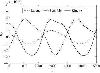
Different energy contributions as a function of time.

2.1 Validation tests
Interparticle force methods such as LBM are known to produce a small-amplitude artificial velocity field around the interface that may introduce significant errors, known as spurious currents (Wagner Reference Wagner2006). The influence of these currents for the present model was investigated by Albernaz et al. (Reference Albernaz, Do-Quang and Amberg2015). By comparing the numerical evaporation rate to the
 $D^{2}$
theoretical law, it was observed that spurious currents may affect the mass flux for droplets with radius
 $R<25$
and interface thickness
 $l>10$
. Therefore, to ensure that mass flux due to numerical errors is negligible, in the present study we have used values of droplet size and interface thickness outside of these ranges.
In a thermodynamic system the temperature can change and phase change may occur. In other words, there is an energy budget in the form of sensible and latent heat, where an estimate of relative importance of these contributions can be useful. In order to quantify and compare different energy budgets, we make use of an oscillating droplet case. A droplet radius
 $R=45$
is considered, for a density ratio
 $\unicode[STIX]{x1D70C}_{\ell }/\unicode[STIX]{x1D70C}_{v}\approx 10$
and a grid size
 $L=256^{3}$
. We proceed with the implementation of a simplified sinusoidal forcing excitation, given as
 $$\begin{eqnarray}F_{T}=a\sin \left[\frac{2\unicode[STIX]{x03C0}x}{L}k_{x}-wt\right],\end{eqnarray}$$
where
 $k_{x}=1$
and
 $w=0.002$
. An amplitude of
 $a=1.6\times 10^{-5}$
is applied, which corresponds to a volume change
 $\unicode[STIX]{x0394}V=\pm 0.015V_{0}$
, where the initial droplet volume is denoted as
 $V_{0}$
. The rate of change of energy due to latent heat can be obtained as
 ${\dot{E}}_{LH}=\unicode[STIX]{x1D6FE}T(\unicode[STIX]{x2202}p/\unicode[STIX]{x2202}T)\dot{V}/V_{0}$
, whereas the energy rate due to sensible heat in the vapour phase is calculated by
 ${\dot{E}}_{S}=\unicode[STIX]{x1D70C}_{v}c_{v}{\dot{T}}$
. Figure 1 shows the different energy rate contributions with time, with the inclusion of the rate of change of kinetic energy for comparison purposes. One can observe that the changes for these budgets have the same order of magnitude, showing that each of these contributions are important for the parameters used. It is important to mention that changes in the droplet volume could also be associated with changes in the liquid density by compressibility effects. The changes in volume
 $\unicode[STIX]{x0394}V$
with respect to the averaged volume
 $\overline{V}$
scales as
 $\unicode[STIX]{x0394}V/\overline{V}=0.037$
, whereas density changes correspond to
 $\unicode[STIX]{x0394}\unicode[STIX]{x1D70C}_{\ell }/\overline{\unicode[STIX]{x1D70C}_{\ell }}=0.0026$
, i.e. more than one order of magnitude difference. Therefore, the volume changes seen in our results are driven mostly by evaporation/condensation events.
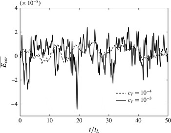
Energy correction as a function of turnover time for different
 $c_{T}$
.

In order to perform an analysis of the turbulent quantities, one needs to first ensure that thermodynamic variables can reach a stationary state. One way to accomplish this when an ideal EOS is used is to directly subtract the energy input
 $E_{cor}=-\unicode[STIX]{x1D70C}\boldsymbol{u}\boldsymbol{\cdot }\boldsymbol{F}_{T}$
in the energy equation (Petersen & Livescu Reference Petersen and Livescu2010). The energy removal can be done uniformly and the mean temperature remains constant for a long run when an ideal EOS is used, even if compressible effects are taken into account (Donzis & Jagannathan Reference Donzis and Jagannathan2013). However, as recently shown by Albernaz et al. (Reference Albernaz, Do-Quang, Hermanson and Amberg2016b
), a correction term based on the control of the pressure is preferable when dealing with non-ideal EOS, especially for conditions close to the critical point where strong fluctuations of thermodynamic quantities are observed. The correction term is uniformly applied all over the domain, given as
 $$\begin{eqnarray}E_{cor}=-c_{T}(\bar{p}-p_{0}),\end{eqnarray}$$
where
 $\bar{p}$
is the mean pressure given for the entire domain and
 $p_{0}$
is the initial saturated reference pressure. The value of
 $E_{cor}$
is updated when the turbulent forcing is changed. The constant
 $c_{T}$
establishes the ‘stiffness’ of the correction, i.e. how fast the system will return to its equilibrium point. The temporal development of the energy correction is shown in figure 2 for different
 $c_{T}$
for
 $Re_{\unicode[STIX]{x1D706}}=91$
with a droplet corresponding to a liquid volume fraction
 $\unicode[STIX]{x1D719}=2.41\,\%$
. We would like to mention that the turbulent quantities are averaged based on the entire domain, i.e. where both phases are considered. Time is normalized by the turbulent eddy turnover time, given as
 $t_{L}=L/\overline{u_{rms}}$
, where
 $\overline{u_{rms}}=\sqrt{2E/3}$
denotes the turbulence intensity. One can observe that the fluctuations for
 $c_{T}=10^{-3}$
are much larger than for
 $c_{T}=10^{-4}$
. Such behaviour is expected since the correction is one order of magnitude higher for the larger value of
 $c_{T}$
and enhances the difference between the averaged pressure in the system to the initial pressure
 $p_{0}$
. However, we have observed that the thermodynamic fluctuations are independent of the value chosen for
 $c_{T}$
. All fluctuations and variances have the same averaged values when long simulations (
 $t/t_{L}>50$
) are considered. Averaging regarding only the liquid phase also shows similar values. Throughout this work
 $c_{T}=10^{-4}$
is used. The average of energy correction for the case shown in figure 2 is
 $\overline{E_{cor}}\approx 5.48\times 10^{-9}$
, for each lattice node, which is equivalent to a temperature of
 $2.5\times 10^{-6}$
K.
3 Turbulence and droplet statistics
In all simulations performed we have considered a relaxation time
 $\unicode[STIX]{x1D70F}_{\unicode[STIX]{x1D708}}=0.5155$
and a grid size
 $L=256^{3}$
. We would like to reiterate that thermodynamic variables are given by their respective reduced values. Characteristic length and time scales are based on grid spacing and time step. Some quantities are scaled by reference values and shown in dimensionless lattice units, standard procedure when solving turbulence by LBM (Qian et al.
Reference Qian, McLaughlin, Sankaranarayanan, Sundaresan and Kontomaris2006; Perlekar et al.
Reference Perlekar, Biferale, Sbragaglia, Srivstava and Toschi2012). In isotropic turbulence simulations, periodic boundary conditions are used in all directions. Initially, the temperature is uniformly defined in the whole domain. In the present simulations, the temperature field is initialized with
 $T_{0}=0.9$
, which gives an equivalent density ratio
 $\unicode[STIX]{x1D70C}_{\ell }/\unicode[STIX]{x1D70C}_{v}\approx 10$
. The corresponding dynamic viscosity ratio is
 $\unicode[STIX]{x1D707}_{\ell }/\unicode[STIX]{x1D707}_{v}\approx 10$
since the phases have same kinematic viscosity. The heat conductivities
 $K_{v}$
and
 $K_{\ell }$
are chosen to match the respective Prandtl numbers for vapour and liquid hexane, which under this temperature are
 $Pr_{v}=0.832$
and
 $Pr_{\ell }=2.253$
(Lemmon, McLinden & Friend Reference Lemmon, McLinden, Friend, Linstrom and Mallard2013).
An initial radius
 $R_{0}$
is chosen for a droplet which is set to equilibrate with the surrounding vapour. When liquid–vapour equilibrium is established and no mass flux takes place, the radius
 $R$
and liquid volume fraction
 $\unicode[STIX]{x1D719}$
are evaluated. The surface tension is calculated based on the Laplace–Young equation at equilibrium and tuned by the parameter
 $\unicode[STIX]{x1D705}$
. The intent is to illustrate the fundamental effects of surface tension, which could be obtained in practice by e.g. additives in the liquid phase. In order to analyse the influence of the surface tension, one can make use of the Ohnesorge number, given as
 $Oh=\unicode[STIX]{x1D707}_{\ell }/(\unicode[STIX]{x1D70C}_{\ell }2R\unicode[STIX]{x1D70E})^{1/2}$
. This dimensionless number is dependent of physical parameters and droplet size only. After equilibrium between the phases is achieved, the stirring force is imposed to generate and sustain turbulence. Thermodynamic variables as well as turbulence characteristics are averaged over both space and time for a time sufficiently long in order to ensure time invariance. The averaging is done for approximately 500 turnover times,
 $t/t_{L}\approx 500$
. Statistics of liquid and vapour phases are performed separately.
In this section, simulations for the same Taylor Reynolds number
 $Re_{\unicode[STIX]{x1D706}}\approx 91$
are shown. The droplet size and Ohnesorge number are changed according to the cases seen in table 1. The turbulent eddy turnover time is approximately
 $t_{L}\approx 6200$
time steps. The Kolmogorov length and time scales assume
 $\unicode[STIX]{x1D702}\approx 1.34$
and
 $t_{\unicode[STIX]{x1D702}}\approx 350$
, respectively. The Taylor length scale is
 $\unicode[STIX]{x1D706}=28$
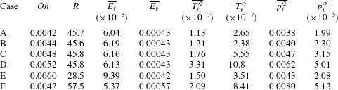
. Cases A–D assume the same droplet size, where the change of surface tension corresponds to different
 $Oh$
. The equivalent liquid volume fraction is
 $\unicode[STIX]{x1D719}\approx 2.41\,\%$
. As a reference in terms of physical units, A–D assume the Kolmogorov scales
 $\unicode[STIX]{x1D702}=2.9~\unicode[STIX]{x03BC}\text{m}$
and
 $t_{\unicode[STIX]{x1D702}}=0.12$
ms for a droplet with a radius
 $R=100~\unicode[STIX]{x03BC}\text{m}$
. The Taylor length scale corresponds to
 $\unicode[STIX]{x1D706}=61.3~\unicode[STIX]{x03BC}\text{m}$
with a turnover time
 $t_{L}=2.2$
ms. For these cases, the kinetic energy of liquid and vapour, denoted respectively as
 $\overline{E_{\ell }}$
and
 $\overline{E_{v}}$
are seen to be insensitive to
 $Oh$
. The thermodynamic variables show however substantial changes. The temperature variance for liquid and vapour raises with increase of
 $Oh$
, i.e. with surface tension decrease. Pressure variances in both phases also increase in the presence of lower surface tension.
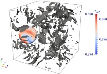
Instantaneous temperature at the droplet surface for
 $Re_{\unicode[STIX]{x1D706}}=91$
and
 $Oh=0.0048$
, where enstrophy isosurfaces are shown for
 $\unicode[STIX]{x1D6FA}/\overline{\unicode[STIX]{x1D6FA}}=3.9$
. The droplet is being translated and deformed by the surrounding vapour phase for a droplet size
 $R=45.8$
(case C).

Parameters values for long-time simulations, for a
 $256^{3}$
grid points mesh with constant Taylor Reynolds number
 $Re_{\unicode[STIX]{x1D706}}\approx 91$
.

An instantaneous temperature field at the droplet surface along with isosurfaces of enstrophy is shown in figure 3 for case C. The enstrophy is defined as
 $\unicode[STIX]{x1D6FA}=\sum _{\boldsymbol{x}}|\unicode[STIX]{x1D735}u|^{2}/L^{3}$
and is normalized by the averaged enstrophy of the flow field
 $\overline{\unicode[STIX]{x1D6FA}}$
. We observe that the temperature varies over the droplet surface, where the droplet shape in this particular instant is nearly spherical. It is important to note that temperature is presented in its reduced value. That said, the instantaneous temperature variation at the droplet surface shown in figure 3 would correspond to 3 K, being significant when phase change is considered.
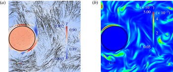
The temperature field for a plane in the
 $x{-}z$
direction is illustrated in figure 4(a), where the solid line identifies the droplet interface. The droplet temperature is higher than that of the surrounding vapour, which shows strong temperature fluctuations only close to the droplet interface. High and low temperature regions may correspond to higher energy dissipation rate
 $\unicode[STIX]{x1D700}$
, which is shown in figure 4(b) for the same plane. It is important to note that energy dissipation rate peaks are not caused only by temperature changes. The velocity vectors are also plotted and one can note that shear layers act at the droplet surface, which may also be associated with energy dissipation.
Plane in the
 $x{-}z$
direction corresponding to figure 3, where (a) shows the temperature field and velocity vectors and (b) the dissipation rate at the same plane. The droplet surface is identified by the solid line.

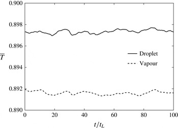
One can also examine the temperature evolution averaged in space for both phases, as shown in figure 5 for case C. The droplet is characterized by a higher temperature than the vapour phase, as observed for the instantaneous field plotted in figure 4(a). The temperature fluctuations are of the same order for both phases, which could be assumed from table 1 due to the similar temperature variance for liquid and vapour phases.
Time evolution of averaged temperature for the droplet and vapour phases.

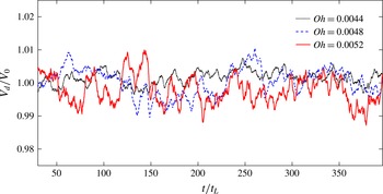
Figure 6 shows the volume of the droplet
 $V_{d}$
as a function of time for different Ohnesorge numbers corresponding to cases B–D. The volume is normalized by the initial volume
 $V_{0}$
, which is nearly the same for all cases. We observe that the decrease (increase) of the droplet volume with time results in phase change where evaporation (condensation) takes place. The amplitudes for these oscillations are dependent on the surface tension. The low surface tension (case D) shows higher amplitude than the larger surface tension (case B) and indicates that significant changes in droplet volume due to phase change are more frequent as surface tension decreases. One should take into consideration that local condensation and evaporation occurrences are dependent on the vapour properties outside the droplet, which change due to the interaction between the liquid and the turbulent eddies in the vapour phase. Higher temperature fluctuations are found for lower surface tension, as observed in table 1, and are therefore responsible for increasing the presence of phase change across the interface. One could also cogitate the importance of thermocapillary effects here. Marangoni forces have been recently investigated by Albernaz et al. (Reference Albernaz, Amberg and Do-Quang2016a
) for a forced convection case. These forces are seen to play a major role when the temperature difference between droplet and surrounding vapour corresponds to
 $\unicode[STIX]{x0394}T=0.1$
. The temperature difference between phases in the present simulations are of the order of
 $\unicode[STIX]{x0394}T\approx 0.005$
(as seen in figure 3). That said, thermocapillary effects do not appear to influence the high temperature fluctuations found for lower surface tension droplets and are hereby neglected.
Temporal development of droplet volume for different surface tensions.

Averaged deformation for different Ohnesorge numbers when
 $Re_{\unicode[STIX]{x1D706}}\approx 91$
and droplet size
 $R\approx 46$
.

The droplet volume behaviour is also expected to be related to the amount of deformation which the droplet experiences, the deformation being another interesting quantity to analyse under different conditions. In order to quantify the droplet deformation, a dimensionless parameter
 $S^{\ast }$
is introduced, defined as
 $$\begin{eqnarray}S^{\ast }=\frac{S-S_{0}}{S_{0}},\end{eqnarray}$$
where
 $S$
is the area of the droplet surface and
 $S_{0}$
the equivalent area of a sphere with the same volume
 $V_{d}$
, i.e.
 $S_{0}=(4\unicode[STIX]{x03C0})^{1/3}(3V_{d})^{2/3}$
. An undeformed droplet would correspond to
 $S^{\ast }=0$
, whereas the amount of deformation grows with
 $S^{\ast }$
. Table 2 shows the averaged droplet deformation
 $\overline{S^{\ast }}$
for different
 $Oh$
, for same droplet size. In order to calculate the droplet deformation, an isosurface has to be generated. The algorithm Marching Cubes is used for this purpose (Lorensen & Cline Reference Lorensen and Cline1987), which is of second-order accuracy. As expected, an increase of deformation is observed when surface tension decreases. The surface tension acts as a restoring force. A strong surface tension produces a scenario where the droplet is not subjected to significant deformations and has as a direct outcome the reduction of phase change events, as previously seen in figure 6.
Different droplet sizes are also investigated as seen in cases E and F, with the same surface tension as case C. In this way, the Ohnesorge number is changed by the droplet size only. We observe that an increase in droplet radius
 $R$
causes a decrease in the kinetic energy of the liquid followed by a growth of vapour kinetic energy. Owing to the fact that
 $Re_{\unicode[STIX]{x1D706}}$
is the same for all cases, i.e. total kinetic energy is maintained, the increase of liquid volume fraction results in an increase (decrease) of the vapour (liquid) kinetic energy. When
 $R=28.5$
(case E), which corresponds to a liquid volume fraction
 $\unicode[STIX]{x1D719}=0.58\,\%$
, the averaged deformation assume the value
 $\overline{S^{\ast }}=6.3\times 10^{-4}$
. Whereas in case F,
 $R=57.5$
(
 $\unicode[STIX]{x1D719}=4.74\,\%$
) gives
 $\overline{S^{\ast }}=0.0032$
. The increase of deformation with droplet size is a consequence of the local Weber number growth, which follows the definition by Perlekar et al. (Reference Perlekar, Biferale, Sbragaglia, Srivstava and Toschi2012) being
 $We_{d}=\unicode[STIX]{x1D70C}_{v}|\boldsymbol{u}_{max,S}-\boldsymbol{u}_{cm}|^{2}(2R)/\unicode[STIX]{x1D70E}$
, where
 $\boldsymbol{u}_{max,S}$
is the maximum velocity at the droplet surface and
 $\boldsymbol{u}_{cm}$
is the velocity of the droplet centre of mass. We would like to mention that the liquid energy dissipation rate
 $\unicode[STIX]{x1D700}_{\ell }$
also grows with droplet size due to the correlation between the droplet dissipation and deformation, investigated in detail on § 5.
We have also investigated the dependence of droplet deformation on the numerical resolution. The idea is to compare the reference case E, where a droplet of
 $R=28.5$
in a
 $L=256^{3}$
grid size is used, to simulations with a grid size
 $L=512^{3}$
and droplet size
 $R=58.2$
. As the box length and droplet radius are twice the reference size, so is the interface thickness. The Taylor Reynolds number obtained is
 $Re_{\unicode[STIX]{x1D706}}=95$
, with a Taylor length
 $\unicode[STIX]{x1D706}=55$
. In this way, the turbulence intensity corresponds to
 $\overline{u_{rms}}=0.0090$
, whereas case E gives
 $\overline{u_{rms}}=0.0169$
. Since fluctuations of thermodynamic quantities are driven by the turbulent intensity (as shown in the next section), different statistics are seen between case E and the higher resolution case. However, the latter shows averaged deformation
 $\overline{S^{\ast }}=6.1\times 10^{-4}$
, which is similar to the deformation obtained in case E. This good agreement supports the use of a space grid
 $L=256^{3}$
throughout the remaining results.
Deformation
 $S^{\ast }$
evolution with time for
 $Re_{\unicode[STIX]{x1D706}}\approx 74$
.

Parameter values and turbulent quantities for long-time simulations with different
 $Re_{\unicode[STIX]{x1D706}}$
. Approximately the same droplet size is used for all cases.

4 The turbulence intensity
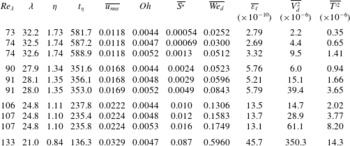
Table 3 lists parameter values where the Taylor Reynolds number and Ohnesorge number are changed. The droplet size
 $R\approx 46$
is used in all cases, which means that
 $Oh$
values change only due to surface tension. The simulations were performed for approximately 600 turnover times with averaging done in both space and time. The averaged Mach number is defined as
 $Ma=\overline{u_{rms}}/c_{s}$
, where the cases shown in table 3 present values in the range
 $0.02<Ma<0.06$
. Turbulence quantities such as the Taylor length scale, Kolmogorov length and time scales are seen to decrease by enhancing
 $Re_{\unicode[STIX]{x1D706}}$
. On the other hand, higher
 $Re_{\unicode[STIX]{x1D706}}$
produces a larger
 $\overline{u_{rms}}$
as well as higher dissipation in the liquid phase. For
 $Re_{\unicode[STIX]{x1D706}}=133$
, the strong turbulence intensity causes droplet breakup, as the droplet diameter is seen to assume values higher than the critical diameter described in (1.1). Detailed investigations on the droplet breakup are out of the scope of this work.
Deformation
 $S^{\ast }$
evolution with time for
 $Re_{\unicode[STIX]{x1D706}}\approx 107$
.

Semi-log probability distribution function of the droplet volume fluctuation
 $V_{d}^{\prime }$
. Different surface tensions are shown with
 $Re_{\unicode[STIX]{x1D706}}\approx 107$
.

We observed that a change in
 $Oh$
for constant
 $Re_{\unicode[STIX]{x1D706}}$
would correspond to fluctuations in the droplet volume (figure 6) and temperature (table 1). In order to quantify the change of these variables according to turbulent effects, table 3 shows the averaged variances of droplet volume and total temperature. As expected, both variances increase by lowering surface tension at a constant
 $Re_{\unicode[STIX]{x1D706}}$
. However, noticeable increase is seen by raising
 $Re_{\unicode[STIX]{x1D706}}$
, which corresponds to two orders of magnitude difference for both variances between
 $Re_{\unicode[STIX]{x1D706}}=74$
and
 $Re_{\unicode[STIX]{x1D706}}=133$
. These observations confirm the strong coupling of turbulence intensity with temperature fluctuations and evaporation/condensation occurrence.
For a given Taylor Reynolds number, the remaining parameters sensitive to changes in the Ohnesorge number (surface tension) are the deformation and
 $We_{d}$
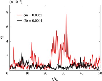
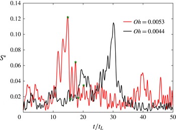
. In figure 7 the deformation evolution for 50 turnover times are shown for
 $Re_{\unicode[STIX]{x1D706}}\approx 74$
. We note that for
 $Oh=0.0052$
(lower surface tension), the events with high peaks are observed, which have magnitude at least four times larger than peaks for
 $Oh=0.0044$
(stronger surface tension case). This is also reflected in the averaged deformation, where
 $\overline{S^{\ast }}=0.0013$
for
 $Oh=0.0052$
and
 $\overline{S^{\ast }}=0.00054$
for
 $Oh=0.0044$
.
The temporal development of deformation for
 $Re_{\unicode[STIX]{x1D706}}\approx 107$
is shown in figure 8 where the overall deformation behaviour is similar for the different Ohnesorge. The high peaks are obtained in both cases, and the average
 $\overline{S^{\ast }}=0.010$
for
 $Oh=0.0044$
is not far from
 $\overline{S^{\ast }}=0.016$
with
 $Oh=0.0053$
. Even though the increase of
 $Re_{\unicode[STIX]{x1D706}}=74$
to
 $Re_{\unicode[STIX]{x1D706}}=107$
may appear to be slight,
 $\overline{u_{rms}}$
is actually two times larger. The outcome is the increase of shear stresses at the droplet interface, resulting in one order of magnitude larger deformation for the same Ohnesorge number. It is important to note that a growth of
 $We_{d}$
is also obtained due to its scaling with the velocity difference squared.
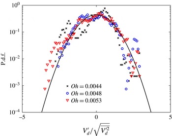
The probability density function (p.d.f.) of the normalized droplet volume fluctuations is shown for different
 $Oh$
in figure 9, for
 $Re_{\unicode[STIX]{x1D706}}\approx 107$
. A first remark is that the p.d.fs follow a Gaussian distribution, shown as the solid line. While a similar trend is seen for the positive fluctuations, the negative fluctuations increase somewhat with lower surface tension, owing to the fact that the occurrence of phase change also increases (figure 6). Such behaviour is also related to the larger temperature variance, where
 $\overline{T_{\ell }^{\prime 2}}=3.22\times 10^{-7}$
and
 $\overline{T_{v}^{\prime 2}}=6.76\times 10^{-7}$
for
 $Oh=0.0044$
whereas
 $\overline{T_{\ell }^{\prime 2}}=9.36\times 10^{-7}$
and
 $\overline{T_{v}^{\prime 2}}=2.37\times 10^{-6}$
for
 $Oh=0.0053$
.
One could also investigate if the droplet shape can present some connection with the respective temperature distribution observed at the surface. Figure 10 shows various droplet deformation shapes at different times, according to symbols found in figure 8, i.e. for
 $Re_{\unicode[STIX]{x1D706}}=107$
and
 $Oh=0.0053$
. We observe that low temperature regions are generally associated with stronger local curvature. Higher temperature at the droplet surface is obtained in regions characterized by flatter surfaces. The local equilibrium provides a relation between curvature and temperature and is analogous to the Gibbs–Thomson effect where small crystals are in equilibrium with the liquid phase at a lower temperature than large crystals due to higher curvature. For a liquid–vapour interface, the equilibrium with higher curvature would correspond to an increase in the vapour pressure (Thomson Reference Thomson1871) and therefore cooling of the droplet surface.
Temperature field at the droplet surface for different deformation values.

Spectrum for temperature with different
 $Re_{\unicode[STIX]{x1D706}}$
.

It is important to note that local temperatures are also dependent on the surrounding flow and thermodynamic conditions, which change especially with higher turbulence intensity and lower droplet surface tension (high
 $Oh$
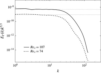
number). Another aspect that can be investigated regarding isotropic turbulence is the well-known result of the energy spectrum. It is expected that the spectrum follows a scaling at the inertial range according to the classical theory of Kolmogorov (Reference Kolmogorov1941). Figure 11 shows the temperature fluctuation spectrum for the entire domain,
 $E_{T}(k)=\sum |T^{\prime 2}(k)|$
. As expected,
 $k^{-5/3}$
scaling is seen to take place at the inertial range. Different
 $Re_{\unicode[STIX]{x1D706}}$
are plotted for same surface tension (
 $Oh\approx 0.0048$
) and it is seen that the temperature spectrum shape is insensitive to
 $Re_{\unicode[STIX]{x1D706}}$
. The kinetic energy spectrum is also shown (figure 12). It is observed that this spectrum also follows a
 $k^{-5/3}$
scaling, where the span of scales in the inertial subrange increases with increasing
 $Re_{\unicode[STIX]{x1D706}}$
.
Turbulent kinetic energy spectrum.

4.1 Correlations
In order to measure the dependence between two variables, a correlation coefficient can be examined. We make use of the Pearson product-moment correlation coefficient
 $r$
, which gives a linear correlation between two variables
 $A$
and
 $B$
and is written as
 $$\begin{eqnarray}r=\langle A,B\rangle =\frac{\text{cov}(A,B)}{s_{A}s_{B}},\end{eqnarray}$$
where
 $\text{cov}$
denotes the covariance and
 $s$
the standard deviation. The correlation
 $r$
can assume values between
 $-1\leqslant r\leqslant 1$
,
 $1$
being a total positive correlation, 0 denoting uncorrelated variables, and
 $-1$
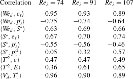
corresponding to a total negative correlation. Table 4 shows the correlations between several quantities as a function of the Taylor Reynolds number. For these correlations a constant Ohnesorge number
 $Oh\approx 0.0048$
and droplet size
 $R\approx 46$
(
 $\unicode[STIX]{x1D719}\approx 2.41\,\%$
) are considered. The dimensionless number
 $We_{d}$
shows a strong correlation with the liquid energy dissipation rate.
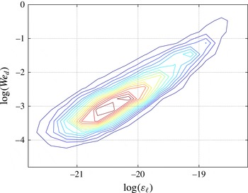
The joint p.d.f. is shown in figure 13, evaluated in a logarithmic scale to better show its behaviour. The contour lines indicate a clear positive correlation and are symmetrically distributed around the maximum probability, which assumes
 $We_{d}=0.5$
and
 $\unicode[STIX]{x1D700}_{\ell }=0.6\times 10^{-9}$
.
Contour lines for the joint p.d.f. of
 $\log (We_{d})$
with
 $\log (\unicode[STIX]{x1D700}_{\ell })$
for
 $Re_{\unicode[STIX]{x1D706}}=107$
. We considered
 $Oh\approx 0.0048$
and
 $R\approx 46$
.

Correlation coefficients for different quantities as a function of
 $Re_{\unicode[STIX]{x1D706}}$
. The same liquid droplet size
 $R\approx 46$
and Ohnesorge number
 $Oh\approx 0.0048$
are used for all cases.

The droplet Weber number is also seen to be positively correlated to the droplet deformation
 $S^{\ast }$
as previously found by Qian et al. (Reference Qian, McLaughlin, Sankaranarayanan, Sundaresan and Kontomaris2006) and Perlekar et al. (Reference Perlekar, Biferale, Sbragaglia, Srivstava and Toschi2012). The parameter
 $We_{d}$
is also correlated negatively with the droplet pressure
 $p_{\ell }^{\prime }$
, slightly weakened by the increase of
 $Re_{\unicode[STIX]{x1D706}}$
. Similar to the
 $We_{d}$
, the deformation parameter
 $S^{\ast }$
is also correlated to
 $\unicode[STIX]{x1D700}_{\ell }$
and negatively correlated to
 $p_{\ell }^{\prime }$
. The increase of deformation would, therefore, dissipate more energy for the liquid phase, whereas the droplet pressure fluctuation decreases. The increase of
 $S^{\ast }$
is also followed by a growth of pressure variance in the vapour phase, which was observed in table 1 and confirmed with the correlation
 $\langle S^{\ast },p_{v}^{\prime 2}\rangle$
. However, it is interesting to observe that this correlation increases with
 $Re_{\unicode[STIX]{x1D706}}$
, where these quantities are uncorrelated when
 $Re_{\unicode[STIX]{x1D706}}=74$
, where
 $r=0.05$
. The growth of temperature variance in the entire domain is also coupled to an increase of the turbulent kinetic energy and is weaker for lower
 $Re_{\unicode[STIX]{x1D706}}$
. The energy dissipation rate and temperature variance are also shown to be relatively correlated and independent of
 $Re_{\unicode[STIX]{x1D706}}$
, which supports observations from figure 4.
As seen in table 4, the fluctuations of the droplet volume and temperature of the entire domain are strongly correlated, where
 $r\approx 0.90$
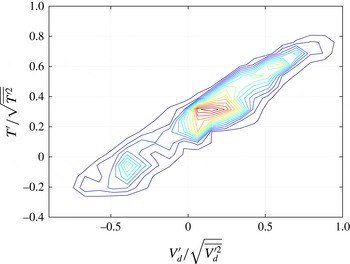
. Figure 14 shows the joint p.d.f. between these quantities for
 $Re_{\unicode[STIX]{x1D706}}=74$
. One should note from the contour lines that the probability shows different peaks, where it is more likely to find a correlation between positive temperature fluctuation with positive
 $V_{d}^{\prime }$
, i.e. when condensation takes place. Evaporation is also correlated to negative temperature fluctuations, however these correlated events are less frequent.
Contour lines for the joint p.d.f. of the temperature fluctuation in the domain
 $T^{\prime }$
with
 $V_{d}^{\prime }$
where
 $Re_{\unicode[STIX]{x1D706}}=74$
. The correlation coefficient is
 $\langle V_{d}^{\prime },T_{v}^{\prime }\rangle =0.96$
.

5 Droplet oscillation frequency
5.1 Droplet released at rest
In order to further investigate the shape evolution of deformed droplets, we have simulated a non-spherical droplet released at rest. Figure 15 shows the deformation parameter
 $S^{\ast }$
as a function of time where an oscillatory behaviour is observed. Due to surface tension forces, the deformation decays with time towards an equilibrium state approaching a spherical shape. Figure 16 illustrates the droplet shape and surface temperature for different time steps. The temperature is uniformly applied as an initial step, where
 $T_{0}=0.9$
. During the shape evolution, it is important to note that flatter regions show higher temperature, as opposed to lower temperatures found on higher curvature regions (as observed in figure 10).
Evolution of droplet deformation for an initial condition
 $S_{0}=0.02$
.

Temperature field at the droplet surface as (a–d)
 $t=0$
,
 $t=8.7\times 10^{3}$
,
 $t=2.3\times 10^{4}$
and
 $t=8.8\times 10^{4}$
. The initial temperature is
 $T_{0}=0.9$
.

Rayleigh (1879) was the first to examine small distortions of drops from equilibrium under the action of forces due to surface tension alone. The frequency
 $f_{d}$
of the
 $n$
th oscillation mode of a liquid drop in air is given by
 $$\begin{eqnarray}f_{d}=\left[\frac{\unicode[STIX]{x1D70E}n(n-1)(n+2)}{(4\unicode[STIX]{x03C0}^{2})\unicode[STIX]{x1D70C}_{\ell }R^{3}}\right]^{1/2}.\end{eqnarray}$$
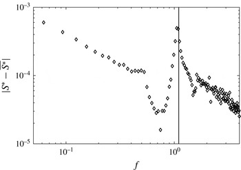
It is important to mention that although (5.1) is a simplified equation which neglects e.g. viscous effects of the droplet and surrounding fluid, it has shown to be sufficient for performing a comparison with our numerical results. A simplified case to analyse the droplet oscillation frequency is to compare the Rayleigh prediction with the non-spherical droplet released at rest. Figure 17 shows the power spectrum corresponding to the deformation parameter
 $|S^{\ast }-\overline{S^{\ast }}|$
obtained from figure 15. Deformation is plotted as a function of frequency
 $f$
(normalized by the time of an oscillation period,
 $t\approx 3100$
). The vertical line corresponds to the frequency predicted by (5.1), for the mode
 $n=2$
. The predicted frequency shows good agreement with the obtained spectrum.
Power spectrum of the deformation parameter corresponding to figure 15.

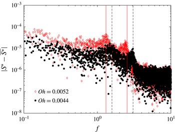
The same comparison can be performed for a droplet in isotropic turbulence. Figure 18 shows the power spectrum of the droplet deformation as a function of frequency
 $f$
(normalized by the sampling rate
 $f_{L}=1/t_{L}$
) for
 $Re_{\unicode[STIX]{x1D706}}=74$
. The vertical lines correspond to the frequencies predicted by (5.1), also normalized with
 $f_{L}$
. The modes
 $n=2$
and
 $n=3$
are plotted in figure 18 for different Ohnesorge numbers, where the solid lines correspond to
 $Oh=0.0052$
and dashed lines to
 $Oh=0.0044$
. The mode
 $n=2$
is the basic oscillatory mode, where the droplet elongates and contracts along the central axis. One should first note that a lower surface tension (
 $Oh=0.0052$
) results in smaller oscillatory frequencies, as indicated in (5.1). The frequency of the peaks from the deformation spectrum show good agreement with the frequency prediction in (5.1).
Power spectrum of the deformation parameter as a function of frequency for
 $Re_{\unicode[STIX]{x1D706}}=74$
.

Power spectrum of the deformation parameter as a function of frequency for
 $Re_{\unicode[STIX]{x1D706}}=91$
.

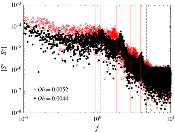
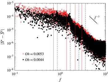
Figures 19 and 20 show the corresponding droplet deformation statistics for a higher Taylor Reynolds number, where the modes of oscillation frequency
 $n=4$
and
 $n=5$
are also included. These figures follow the same range of scaling in
 $x{-}y$
axes as used in figure 18. We observe that the power spectrum increases its magnitude with
 $Re_{\unicode[STIX]{x1D706}}$
due to the higher deformations. It is also seen that larger
 $Re_{\unicode[STIX]{x1D706}}$
highlights different oscillation modes, especially when
 $Re_{\unicode[STIX]{x1D706}}=91$
. However, in the case where
 $Re_{\unicode[STIX]{x1D706}}=107$
the modes are not distinct, even for
 $n=2$
. The amount of nonlinearity in the oscillations due to the strong turbulence brings forward different frequencies, which overlap each other and shows a more continuous spectrum. This is opposite to figure 18 where these intermediate frequencies are damped and a clear separation of the basic modes could be observed.
Power of the deformation parameter as a function of frequency for
 $Re_{\unicode[STIX]{x1D706}}=107$
.

One should note that for
 $Oh\approx 0.0052$
, while
 $f_{d}(n=2)\approx 1.3$
when
 $Re_{\unicode[STIX]{x1D706}}=74$
, the frequency changes to
 $f_{d}(n=2)\approx 0.7$
for
 $Re_{\unicode[STIX]{x1D706}}=107$
. This is due to the fact that
 $f$
is scaled with the eddy turnover time
 $t_{L}$
. The difference in frequency can also be observed in figures 7 and 8, which correspond to the cases,
 $Re_{\unicode[STIX]{x1D706}}=74$
and
 $Re_{\unicode[STIX]{x1D706}}=107$
, respectively. The scaled frequency of oscillations decreases with the Taylor Reynolds number, exhibiting the same relation as the frequency change, i.e. almost two times smaller in figure 8 when compared with figure 7. Another aspect worth mentioning is the decay found in figure 20: although oscillatory modes are difficult to be discerned, there is an evident decrease between frequencies
 $1.5<f<8$
, which follows an approximate fit that scales
 ${\sim}f^{-3}$
.
6 Conclusions
We have studied the dynamics of a droplet surrounded by its own vapour in isotropic turbulence, where heat and mass transfer have been considered. A density ratio
 $\unicode[STIX]{x1D70C}_{\ell }/\unicode[STIX]{x1D70C}_{v}\approx 10$
is used, which corresponds to a hexane fluid with a reduced temperature value of
 $T=0.9$
. Numerical simulations are performed with a lattice Boltzmann hybrid scheme, where phase separation is controlled by a non-ideal equation of state. We have proposed a pressure control so that an equilibrium condition with a stationary state for the thermodynamic quantities could be obtained.
The primary focus has been to analyse the coupling between turbulence parameters, thermodynamic variables and droplet dynamics. Fluctuations of thermodynamic and turbulence variables are averaged separately for the liquid and vapour phases. Droplet statistics are described in terms of a dimensionless deformation parameter
 $S^{\ast }$
, the droplet volume and a local Weber number. The change in surface tension can be quantified by the Ohnesorge number, for a constant droplet size. The droplet is carried by the surrounding vapour, which moves faster due to its lower density. Deformation is caused by the shear stresses at the droplet interface and increases with
 $Re_{\unicode[STIX]{x1D706}}$
. The droplet volume shows fluctuations which correspond to the presence of evaporation/condensation. The amount of phase change is directly related to the surface tension and thermodynamic fluctuations: lower surface tension produces a growth in thermodynamic fluctuations and increases the phase change. The local equilibrium at the droplet surface shows low temperature regions associated with stronger curvature whereas higher temperature is obtained in flatter surface regions.
As expected, the amount of deformation grows with lower surface tensions and larger droplet size: the Weber number explains this increase and is correlated to
 $S^{\ast }$
. We have also focused on the effects of turbulent quantities and the energy spectra for different
 $Re_{\unicode[STIX]{x1D706}}$
. An interesting behaviour is observed for the deformation evolution as Ohnesorge number (surface tension) is changed for different
 $Re_{\unicode[STIX]{x1D706}}$
. Distinct peaks are present only for the lower surface tension case with
 $Re_{\unicode[STIX]{x1D706}}\approx 74$
(figure 7), and are not obtained for
 $Re_{\unicode[STIX]{x1D706}}\approx 107$
(figure 8). This is reflected in the averaged quantities of
 $S^{\ast }$
and
 $We_{d}$
which show changes for lower
 $Re_{\unicode[STIX]{x1D706}}$
as seen in table 3. One could also observe that the turbulence quantities are insensitive to surface tension changes.
The oscillation frequency of the droplet has been investigated and compared to classical predictions by Rayleigh. The basic modes of oscillation
 $n=2$
and
 $n=3$
could be identified for
 $Re_{\unicode[STIX]{x1D706}}=74$
(figure 18). With an intermediate
 $Re_{\unicode[STIX]{x1D706}}=91$
(figure 19), more modes are present. However, with
 $Re_{\unicode[STIX]{x1D706}}=107$
these are replaced by a continuous spectrum, showing a decrease that scales as
 ${\sim}f^{-3}$
. Correlation coefficients are also calculated, where
 $We_{d}$
is strongly correlated with the liquid energy dissipation rate (figure 13). Weber number also shows correlation with
 $S^{\ast }$
as found by different authors, and a negative correlation to the fluid pressure fluctuations
 $p_{\ell }^{\prime }$
. A strong correlation is seen for the fluctuations of droplet volume and vapour temperature, which are more likely to happen between positive temperature fluctuation and droplet condensation, as shown in the joint probability distribution function in figure 14. This result confirms that phase change is coupled to temperature fluctuations.
Acknowledgements
This work was supported by the Swedish Research Council (VR2010-3938 and VR2011-5355). We acknowledge computational support from the Swedish National Infrastructure for Computing (SNIC) and the pan-European HPC Research Infrastructure (PRACE-3IP, project FP7 RI-312763).