1 Introduction
Thin glass sheets are increasingly prevalent in everyday technology, with current applications including substrates in thin-film batteries and thumbprint sensors in smartphones, and with futuristic applications such as bendable televisions and tablets on the horizon (Burke Reference Burke2016; Horvatitsch Reference Horvatitsch2016). Specialist thin glass sheets are often manufactured using a ‘redraw’ process, whereby a prefabricated block is fed continuously into a furnace (referred to as a heater zone) where it is heated and stretched by the application of draw rollers downstream. During the redraw process, out-of-plane ripples sometimes develop in the glass sheet which persist downstream of the heater zone and draw rollers, and render the product unusable. The source of these ripples is not immediately obvious, and the extreme temperatures required for the manufacturing process make in situ imaging of ripple formation very difficult.
Glass drawing processes are characterized by the small ratio of thickness (or radius) to other length scales, and reduced models exploit this small parameter (see, for example, Matovich & Pearson Reference Matovich and Pearson1969). An early study of viscous buckling was presented by Taylor (Reference Taylor1969), whose experiments include a viscous thread floating on mercury which buckles when its ends are pushed together. Buckmaster, Nachman & Ting (Reference Buckmaster, Nachman and Ting1975) modelled the buckling and demonstrated the emergence of a new time scale associated with buckling which is shorter than the time scale for stretching. Later, Howell (Reference Howell1994, Reference Howell1996) noted that even small inertial effects dramatically change the behaviour, and a buckling length scale shorter than the sheet length must also be introduced. The buckling of a thin viscous sheet or fibre has since been studied extensively due to its prevalence in everyday life (e.g. honey coiling, Mahadevan, Ryu & Samuel Reference Mahadevan, Ryu and Samuel1998), industrial manufacturing processes (Batty et al. Reference Batty, Uribe, Audoly and Grinspun2012; Perdigou Reference Perdigou2015), and geophysical flows (Ribe Reference Ribe2001).
A substantial body of work has been developed describing the buckling of a viscous sheet or jet impinging on a perpendicular plate following the experimental study of Cruickshank & Munson (Reference Cruickshank and Munson1981), who measured the periods of folding and coiling of thin sheets and jets of viscous fluid and recorded the increase of folding/coiling frequency with the length of the falling jet. Cruickshank (Reference Cruickshank1988) and Tchavdarov, Yarin & Radev (Reference Tchavdarov, Yarin and Radev1993) developed mathematical models for this buckling phenomenon and predicted the heights at which a plane jet and an axisymmetric jet become unstable along with the corresponding period of folding/coiling. Chiu-Webster & Lister (Reference Chiu-Webster and Lister2006) and Morris et al. (Reference Morris, Dawes, Ribe and Lister2008) modified the standard impinging-jet experiments to observe a falling jet impinging on a perpendicular moving belt, so that the jet is draped along the surface. The unstable buckling modes depend on the fall height, belt speed and viscosity, and the large range of observed modes has caused the apparatus to be dubbed a ‘fluid-mechanical sewing machine’.
In the context of thin glass sheets, the presence of buckling or ripples is highly undesirable, motivating an investigation of the production of ripples during glass drawing. A model for the viscous flow of a three-dimensional sheet in the small-aspect-ratio limit was derived by Howell (Reference Howell1994, Reference Howell1996), who used this as a model for the float-glass process. This thin-sheet model has been used to characterize the thickness profile of a redrawn glass sheet by Filippov & Zheng (Reference Filippov and Zheng2010) and by O’Kiely et al. (Reference O’Kiely, Breward, Griffiths, Howell and Lange2015, Reference O’Kiely, Breward, Griffiths, Howell and Lange2018). Filippov & Zheng (Reference Filippov and Zheng2010) noted that the instability of a stretched thin viscous sheet is linked to the existence of compressive zones in the sheet, and calculated these zones for a glass sheet undergoing redraw. More recently, Srinivasan, Wei & Mahadevan (Reference Srinivasan, Wei and Mahadevan2017) and O’Kiely (Reference O’Kiely2018) solved the linear-stability problem for small out-of-plane deformations, determining the fastest-growing eigenmodes and corresponding growth rates for early-time growth of ripples in sheets, and investigated the dependence of the buckling behaviour on the length of the heater zone through which the sheet is drawn. They determined that compressive buckling zones are always present upstream of the stretching region, and that short heater zones give rise to a second buckling region downstream of the stretching region.
The results of Filippov & Zheng (Reference Filippov and Zheng2010) and Srinivasan et al. (Reference Srinivasan, Wei and Mahadevan2017) are based on first solving the in-plane problem to determine the stress in a three-dimensional glass sheet undergoing redraw, and then analysing the transverse stability of the sheet subject to the given stress profile. Therefore they do not capture the subsequent nonlinear buckling behaviour, during which the in-plane stress and out-of-plane deformation are coupled. Our aim in this paper is to study this coupling in the simpler context of a two-dimensional thin viscous sheet undergoing redraw under gravity, and to determine when and how it will buckle.
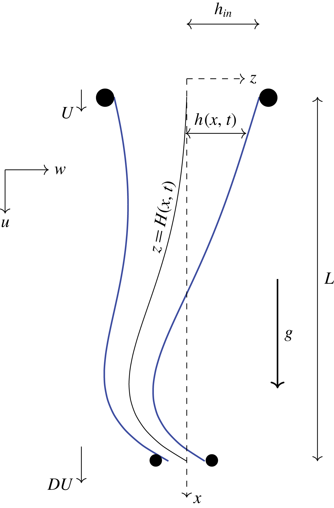
The stress in a two-dimensional sheet undergoing downwards redraw (as shown schematically in figure 1) is a combination of the tension due to the downstream rollers and the compressive stress caused by gravity. When the effect of gravity is relatively small, the sheet experiences a positive tension everywhere. As the effect of gravity is increased, the sheet velocity increases beyond the draw velocity, the tension changes sign in some region of the sheet, and an instability occurs. Since the sheet cannot escape through the draw rollers as quickly as it arrives, its centreline increases in length and buckles out of plane. Since the transverse deformation, in turn, modifies the tension/compression in the sheet, the location of any compressive zone is not determined a priori but must be computed along with the centreline dynamics. In this scenario, the location of the sheet centreline at the top and bottom of the heater zone is fixed by rollers, in contrast with the studies carried out by authors such as Cruickshank & Munson (Reference Cruickshank and Munson1981), in which the point of contact of the sheet (or jet) is free to move across a perpendicular surface.
The plan for this paper is as follows. In § 2 we present a mathematical model for the dynamics of a two-dimensional thin glass sheet buckling due to gravity while undergoing redraw. In § 3 we determine the steady-state solution, and investigate the effect of process parameters on centreline stability. In § 4 we present numerical solutions of our simplified model, and an early-time linear-stability analysis, while in § 5 we analyse the late-time behaviour. Finally, in § 6 we discuss our findings and their implications for a more general study of buckling processes in thin viscous sheets.
2 Model derivation
2.1 Full dimensional model
The complexity of the mathematical model governing the centreline deformation of a viscous sheet or thread depends on the size of the deformation. To describe deformations that are comparable with the sheet length, a geometrically nonlinear model is necessary (Buckmaster et al. Reference Buckmaster, Nachman and Ting1975). In this paper, we focus on the simpler case where the centreline deformation is comparable to the thickness and the sheet is approximately planar; we assess the validity of this assumption in § 5.6.
Two-dimensional glass sheet with thickness
 $2h(x,t)$
undergoing drawing over a distance
 $L$
in the
 $x$
-direction subject to gravity
 $g$
, also acting in the
 $x$
-direction. The sheet has velocity
 $\boldsymbol{u}=(u,w)$
with feed speed
 $u=U$
and draw speed
 $u=DU$
, and centreline
 $z=H(x,t)$
, and
 $h(0,t)=h_{in}=$
is a prescribed constant.

We consider a two-dimensional (infinitely wide) nearly planar sheet, and use Cartesian coordinates
 $\boldsymbol{x}=(x,z)$
, with the
 $x$
-axis aligned with the direction of drawing and
 $z$
in the transverse direction, as shown in figure 1. We consider a sheet with thickness
 $2h(x,t)$
, which undergoes drawing over a distance
 $L$
in the
 $x$
-direction, with gravity also acting in the positive
 $x$
-direction. We use the notation
 $h(0,t)=h_{in}$
for the initial half-thickness,
 $U$
for the feed speed and
 $DU$
for the draw speed. We denote the sheet centreline by
 $H(x,t)$
, so that the glass surfaces are located at
 $z=z^{\pm }(x,t):=H(x,t)\pm h(x,t)$
for
 $0<x<L$
.
We assume the glass is an incompressible Newtonian fluid and is therefore governed by the Navier–Stokes equations
 $$\begin{eqnarray}\unicode[STIX]{x1D735}\boldsymbol{\cdot }\boldsymbol{u}=0,\quad \unicode[STIX]{x1D70C}\frac{\text{D}\boldsymbol{u}}{\text{D}t}=\unicode[STIX]{x1D735}\boldsymbol{\cdot }\unicode[STIX]{x1D748}+\unicode[STIX]{x1D70C}g\hat{\boldsymbol{\imath }}.\end{eqnarray}$$
Here
 $\boldsymbol{u}=(u,w)$
is the velocity vector,
 $\unicode[STIX]{x1D735}=(\unicode[STIX]{x2202}/\unicode[STIX]{x2202}x,\unicode[STIX]{x2202}/\unicode[STIX]{x2202}z)$
is the two-dimensional gradient operator,
 $\text{D}/\text{D}t=\unicode[STIX]{x2202}/\unicode[STIX]{x2202}t+\boldsymbol{u}\boldsymbol{\cdot }\unicode[STIX]{x1D735}$
is the convective derivative and
 $\hat{\boldsymbol{\imath }}$
is a unit vector in the
 $x$
-direction. The stress tensor is given by
 $$\begin{eqnarray}\unicode[STIX]{x1D748}=-p\mathbb{I}+\unicode[STIX]{x1D707}\left(\unicode[STIX]{x1D735}\boldsymbol{u}+(\unicode[STIX]{x1D735}\boldsymbol{u})^{\text{T}}\right),\end{eqnarray}$$
with
 $p$
denoting pressure,
 $\mathbb{I}$
the identity matrix and
 $\unicode[STIX]{x1D707}$
the viscosity. Glass has a strongly temperature-dependent viscosity, which varies during the redraw process as the sheet is heated and cooled. However, our focus here is on the fundamental fluid-mechanical processes involved in buckling, and we assume for simplicity that the sheet has uniform viscosity.
On the free surfaces
 $z=z^{\pm }$
, we impose kinematic and no-stress conditions
 $$\begin{eqnarray}\frac{\text{D}}{\text{D}t}(z-z^{\pm })=0,\quad \unicode[STIX]{x1D748}\boldsymbol{\cdot }\hat{\boldsymbol{n}}=\mathbf{0},\end{eqnarray}$$
where
 $\hat{\boldsymbol{n}}$
is the unit vector normal to the free surface. We neglect the effect of surface tension under the assumption that the capillary number
 $Ca=\unicode[STIX]{x1D707}U/\unicode[STIX]{x1D6FE}\gg 1$
, where
 $\unicode[STIX]{x1D6FE}$
is surface tension (typically
 $Ca\approx 10^{2}$
).
Appropriate boundary conditions to be imposed at the inlet
 $x=0$
and at the outlet
 $x=L$
will be discussed later after we have reduced the problem to a thin-sheet model. We also need initial conditions for this time-dependent problem, and we will discuss how these may be chosen in § 3.
2.2 Non-dimensionalization
We define the aspect ratio of the sheet,
 $\unicode[STIX]{x1D716}$
, by
 $$\begin{eqnarray}\unicode[STIX]{x1D716}=\frac{\text{inlet half-thickness}}{\text{length of drawing process}}=\frac{h_{in}}{L}.\end{eqnarray}$$
The thickness is always much smaller than the length in glass drawing processes, so we assume that
 $\unicode[STIX]{x1D716}\ll 1$
.
We also define the Reynolds number
 $Re=\unicode[STIX]{x1D70C}LU/\unicode[STIX]{x1D707}$
. In industrial processes of interest, the Reynolds number is invariably small (
 $Re\lesssim 10^{-4}$
), but inertia terms may be important if buckling takes place over a sufficiently short time scale. In particular, scaling arguments in Howell (Reference Howell1996) predict that the length scale and time scale associated with buckling are
 $$\begin{eqnarray}\text{length scale}\sim \unicode[STIX]{x1D716}^{2/3}Re^{-1/6}L,\quad \text{time scale}\sim \unicode[STIX]{x1D716}^{2/3}Re^{1/3}\frac{L}{U},\end{eqnarray}$$
if the Reynolds number is
 $O(\unicode[STIX]{x1D716}^{4})$
or larger. We focus on the distinguished limit where
 $Re=O(\unicode[STIX]{x1D716}^{4})$
so that, according to (2.5), the buckling wavelength is comparable to the heater length
 $L$
and the time scale is of order
 $\unicode[STIX]{x1D716}^{2}L/U$
. This choice results in a canonical model in which inertia plays a role at leading order, and limiting versions of which apply to the cases when
 $Re\ll \unicode[STIX]{x1D716}^{4}$
or
 $\unicode[STIX]{x1D716}^{4}\ll Re\ll 1$
.
Bearing in mind the above scaling arguments, we non-dimensionalize our model using
 $$\begin{eqnarray}\displaystyle & \displaystyle (x^{\prime },z^{\prime })=\frac{(x,\unicode[STIX]{x1D716}^{-1}z)}{L},\quad (u^{\prime },w^{\prime })=\frac{(u,\unicode[STIX]{x1D716}w)}{U},\quad t^{\prime }=\frac{t}{\unicode[STIX]{x1D716}^{2}L/U}, & \displaystyle\end{eqnarray}$$
 $$\begin{eqnarray}\displaystyle & \displaystyle (h^{\prime },H^{\prime },z^{\pm ^{\prime }})=\frac{(h,H,z^{\pm })}{\unicode[STIX]{x1D716}L},\quad (p^{\prime },\unicode[STIX]{x1D70E}_{xx}^{\prime },\unicode[STIX]{x1D70E}_{xz}^{\prime },\unicode[STIX]{x1D70E}_{zz}^{\prime })=\frac{(p,\unicode[STIX]{x1D70E}_{xx},\unicode[STIX]{x1D716}^{-1}\unicode[STIX]{x1D70E}_{xz},\unicode[STIX]{x1D716}^{-2}\unicode[STIX]{x1D70E}_{zz})}{\unicode[STIX]{x1D707}U/L}. & \displaystyle\end{eqnarray}$$
With primes dropped, the Navier–Stokes equations (2.1) in dimensionless form become
 $$\begin{eqnarray}\displaystyle & \displaystyle \unicode[STIX]{x1D716}^{2}u_{x}+w_{z}=0, & \displaystyle\end{eqnarray}$$
 $$\begin{eqnarray}\displaystyle & \displaystyle (\unicode[STIX]{x1D70E}_{xx})_{x}+(\unicode[STIX]{x1D70E}_{xz})_{z}+St=\unicode[STIX]{x1D716}^{2}\widehat{Re}\left(u_{t}+\unicode[STIX]{x1D716}^{2}uu_{x}+wu_{z}\right), & \displaystyle\end{eqnarray}$$
 $$\begin{eqnarray}\displaystyle & \displaystyle (\unicode[STIX]{x1D70E}_{xz})_{x}+(\unicode[STIX]{x1D70E}_{zz})_{z}=\widehat{Re}\left(w_{t}+\unicode[STIX]{x1D716}^{2}uw_{x}+ww_{z}\right), & \displaystyle\end{eqnarray}$$
 $Re/\unicode[STIX]{x1D716}^{4}=\widehat{Re}=O(1)$
, and the Stokes number
 $$\begin{eqnarray}St=\frac{\unicode[STIX]{x1D70C}gL^{2}}{\unicode[STIX]{x1D707}U}\end{eqnarray}$$
gives the ratio of gravity to viscous forces. The components of the Newtonian constitutive relation (2.2) read
 $$\begin{eqnarray}\unicode[STIX]{x1D70E}_{xx}=-p+2u_{x},\quad \unicode[STIX]{x1D716}^{2}\unicode[STIX]{x1D70E}_{xz}=u_{z}+w_{x},\quad \unicode[STIX]{x1D716}^{2}\unicode[STIX]{x1D70E}_{zz}=-p-2u_{x},\end{eqnarray}$$
and the dimensionless versions of the free-surface boundary conditions (2.3) are
 $$\begin{eqnarray}w=z_{t}^{\pm }+\unicode[STIX]{x1D716}^{2}uz_{x}^{\pm },\quad \unicode[STIX]{x1D70E}_{xz}=z_{x}^{\pm }\unicode[STIX]{x1D70E}_{xx},\quad \unicode[STIX]{x1D70E}_{zz}=z_{x}^{\pm }\unicode[STIX]{x1D70E}_{xz}\end{eqnarray}$$
at
 $z=z^{\pm }(x,t)$
.
Before proceeding with the asymptotic analysis, we first derive some exact conservation principles by integrating the governing equations (2.7) across the sheet thickness. First by integrating (2.7a
) from
 $z=z^{-}$
to
 $z=z^{+}$
and applying the boundary condition (2.10 a
), we obtain the net mass-conservation equation
 $$\begin{eqnarray}h_{t}+\unicode[STIX]{x1D716}^{2}(h\overline{u})_{x}=0,\end{eqnarray}$$
where the bar denotes the cross-sectional average
 $$\begin{eqnarray}\overline{f}(x,t)=\frac{1}{2h(x,t)}\int _{z^{-}(x,t)}^{z^{+}(x,t)}f(x,z,t)\,\text{d}z.\end{eqnarray}$$
Similarly, integration of (2.7b
) and (2.7c
) with respect to
 $z$
and application of (2.10a-c
) results in
 $$\begin{eqnarray}\displaystyle & \displaystyle \left(h\overline{\unicode[STIX]{x1D70E}}_{xx}\right)_{x}+Sth=\unicode[STIX]{x1D716}^{2}\widehat{Re}[(h\overline{u})_{t}+\unicode[STIX]{x1D716}^{2}\big(h\overline{u^{2}}\big)_{x}], & \displaystyle\end{eqnarray}$$
 $$\begin{eqnarray}\displaystyle & \displaystyle \left(h\overline{\unicode[STIX]{x1D70E}}_{xz}\right)_{x}=\widehat{Re}[\left(h\overline{w}\right)_{t}+\unicode[STIX]{x1D716}^{2}\left(h\overline{uw}\right)_{x}], & \displaystyle\end{eqnarray}$$
 $x$
- and
 $z$
-directions.
Finally, we obtain a net moment balance by multiplying (2.7b
) by
 $(z-H)$
before integrating across the sheet with respect to
 $z$
, resulting in
 $$\begin{eqnarray}\left[h\overline{(z-H)\unicode[STIX]{x1D70E}_{xx}}\right]_{x}+H_{x}h\overline{\unicode[STIX]{x1D70E}}_{xx}-h\overline{\unicode[STIX]{x1D70E}}_{xz}=\frac{\unicode[STIX]{x1D716}^{2}\widehat{Re}}{2}\int _{z^{-}}^{z^{+}}(z-H)\left(u_{t}+\unicode[STIX]{x1D716}^{2}uu_{x}+wu_{z}\right)\!\text{d}z.\end{eqnarray}$$
2.3 Thin-sheet limit
Now we are ready to let
 $\unicode[STIX]{x1D716}\rightarrow 0$
in the governing equations and boundary conditions (2.7)–(2.14). From (2.7a
) we see that
 $w$
is independent of
 $z$
to leading order, and the kinematic boundary conditions (2.10 a
) then imply that
 $$\begin{eqnarray}w=H_{t}\end{eqnarray}$$
and
 $$\begin{eqnarray}h_{t}=0,\end{eqnarray}$$
so the sheet thickness remains fixed over the buckling time scale. The thickness profile is therefore given by the initial conditions, which we discuss in § 3.
The leading-order velocity and axial stress are then determined from (2.9) as
 $$\begin{eqnarray}u=\overline{u}+(H-z)H_{xt},\quad \unicode[STIX]{x1D70E}_{xx}=4u_{x}.\end{eqnarray}$$
We can thus evaluate the relevant integrals of
 $\unicode[STIX]{x1D70E}_{xx}$
in (2.13a
) and (2.14) to obtain
 $$\begin{eqnarray}h\overline{\unicode[STIX]{x1D70E}}_{xx}=4h(\overline{u}_{x}+H_{x}H_{xt}),\quad h\overline{(z-H)\unicode[STIX]{x1D70E}_{xx}}=-\frac{4h^{3}}{3}H_{xxt}.\end{eqnarray}$$
These two quantities describe the axial tension and the bending moment in the sheet, respectively with the factor of
 $4h^{3}/3$
representing the dimensionless bending stiffness.
Finally, by eliminating
 $\overline{\unicode[STIX]{x1D70E}}_{xz}$
from the averaged equations (2.13b
) and (2.14), we obtain the leading-order system
 $$\begin{eqnarray}\displaystyle & \displaystyle [4h(\overline{u}_{x}+H_{x}H_{xt})]_{x}=-St\,h, & \displaystyle\end{eqnarray}$$
 $$\begin{eqnarray}\displaystyle & \displaystyle \widehat{Re}\,h\,H_{tt}+\left(\frac{4h^{3}}{3}H_{xxt}\right)_{xx}=[4h(\overline{u}_{x}+H_{x}H_{xt})H_{x}]_{x}. & \displaystyle\end{eqnarray}$$
 $4h(\overline{u}_{x}+H_{x}H_{xt})$
on the left-hand side of (2.19a
) is the viscous tension in the sheet. The same term appears on the right-hand side of (2.19b
), where it may act to straighten or bend the sheet, depending on whether it is positive or negative. On the left-hand side of (2.19b
), the first term corresponds to the inertia of the sheet, and the expression inside the brackets of the second term is the bending moment.
With
 $h(x)$
in principle a known function, (2.19) gives a coupled system of partial differential equations for
 $\overline{u}(x,t)$
and
 $H(x,t)$
. In addition to two initial conditions for
 $H$
, to be discussed below, the system requires one boundary condition for
 $u$
and two boundary conditions for
 $H$
at each end of the domain
 $x=0$
and
 $x=1$
. We have non-dimensionalized with the inlet flow speed and therefore impose
 $$\begin{eqnarray}u(0,t)=1,\quad u(1,t)=D,\end{eqnarray}$$
where the draw ratio
 $D$
is the ratio of the draw speed to the inlet speed. For the centreline deformation, we suppose that the transverse deflection is constrained to be zero by the inlet and outlet rollers, and that no bending moment is imposed at either end, which implies the simple-support boundary conditions
 $$\begin{eqnarray}H(0,t)=H_{xxt}(0,t)=0,\quad H(1,t)=H_{xxt}(1,t)=0.\end{eqnarray}$$
By integrating (2.19a
) with respect to
 $x$
, we can express the tension in the sheet as
 $$\begin{eqnarray}4h(\bar{u}_{x}+H_{x}H_{xt})=St\int _{x}^{1}h(s)\,\text{d}s+c(t),\end{eqnarray}$$
where
 $c(t)$
is the force on the sheet at
 $x=1$
. If
 $c(t)<0$
then this force is in the upward direction, so some portion of the sheet near
 $x=1$
is under compression and we expect the centreline to be susceptible to buckling. Integrating (2.22) and applying boundary conditions (2.20), we can express
 $c$
in terms of the as yet unknown centreline deflection:
 $$\begin{eqnarray}c(t)=\left.\left[D-1-\frac{St}{4}\int _{0}^{1}\int _{x}^{1}\frac{h(s)}{h(x)}\,\text{d}s\,\text{d}x+\int _{0}^{1}H_{x}(x,t)H_{xt}(x,t)\,\text{d}x\right]\right/\int _{0}^{1}\frac{\text{d}x}{4h(x)}.\end{eqnarray}$$
We obtain a single non-local equation for
 $H(x,t)$
by substituting (2.22) into the moment balance (2.19b
) to give
 $$\begin{eqnarray}\widehat{Re}\,h\,H_{tt}+\left(\frac{4h^{3}}{3}H_{xxt}\right)_{xx}=\left[\left(St\int _{x}^{1}h(s)\,\text{d}s+c(t)\right)H_{x}\right]_{x}.\end{eqnarray}$$
The evolution of the sheet centreline is governed by equation (2.24), with
 $c(t)$
determined by (2.23), subject to the boundary conditions (2.21) and suitable initial conditions. We note that this model breaks down once the centreline deformation is large enough that
 $H_{xx}=O(1/\unicode[STIX]{x1D716})$
. Once this regime is reached, the centreline deformation should be scaled with the sheet length rather than its thickness, and additional geometrical nonlinearities are promoted into the leading-order governing equations (Howell Reference Howell1994, Chapter 3).
3 Initial conditions and stability
If the sheet centreline is stable, then the sheet remains flat, and its thickness and in-plane velocity evolve on the stretching time scale which is much longer than the buckling time scale; we see that a balance occurs in the exact mass-conservation equation (2.11) when
 $t=O(\unicode[STIX]{x1D716}^{-2})$
. On the other hand, for some parameter values the sheet centreline becomes unstable and then evolves on the fast buckling time scale. In this unstable regime, the initial conditions for the buckling problem are given by the solution on the stretching time scale at the time at which the sheet first becomes unstable. The initial conditions therefore depend on the route by which the system approaches the unstable regime. We consider an idealized scenario in which the sheet is initially held fixed and the thickness and velocity are in steady state. At
 $t=0$
, the centreline is released and the sheet can undergo buckling.
Under this assumption, the thickness and initial velocity are given by the solution to the steady-state versions of (2.11) and (2.19) with
 $H\equiv 0$
, i.e.
 $$\begin{eqnarray}\overline{u}h=1,\quad (4h\overline{u}_{x})_{x}=-St\,h,\end{eqnarray}$$
with boundary conditions
 $$\begin{eqnarray}\overline{u}(0)=h(0)=1,\quad \bar{u}(1)=D.\end{eqnarray}$$
We note that this is the standard steady-state Trouton model for one-dimensional viscous stretching with gravity (Howell Reference Howell1994). The solutions to (3.1), (3.2) are given by
 $$\begin{eqnarray}\displaystyle & \displaystyle \overline{u}(x)=\left(\frac{St}{2a}\right)\sin ^{2}\left(\frac{\sqrt{a}}{2}x+\sin ^{-1}\sqrt{\frac{2a}{St}}\right), & \displaystyle\end{eqnarray}$$
 $$\begin{eqnarray}\displaystyle & \displaystyle h(x)=\left(\frac{2a}{St}\right)\operatorname{cosec}^{2}\left(\frac{\sqrt{a}}{2}x+\sin ^{-1}\sqrt{\frac{2a}{St}}\right), & \displaystyle\end{eqnarray}$$
 $a<St/2$
satisfies the transcendental equation
 $$\begin{eqnarray}D=\left(\frac{St}{2a}\right)\sin ^{2}\left(\frac{\sqrt{a}}{2}+\sin ^{-1}\sqrt{\frac{2a}{St}}\right).\end{eqnarray}$$
The initial profile is unstable whenever any portion of the sheet is under compression. This assertion can be verified by solving the linear stability problem outlined in § 4.1, and is consistent with analogous wrinkling problems in thin elastic sheets, which cannot sustain a compressive force in the ‘high-bendability’ limit (see, for example, Davidovitch et al.
Reference Davidovitch, Schroll, Vella, Adda-Bedia and Cerda2011). Compression is most likely to occur near
 $x=1$
, since the positive contribution to the tensile force (the integral term in (2.24)) is zero there. At
 $x=1$
, the force on the sheet is given by
 $$\begin{eqnarray}\displaystyle c & = & \displaystyle \left.\left[D-1-\frac{St}{4}\int _{0}^{1}\int _{x}^{1}\frac{h(s)}{h(x)}\,\text{d}s\,\text{d}x\right]\right/\int _{0}^{1}\frac{\text{d}x}{4h(x)}\nonumber\\ \displaystyle & = & \displaystyle 4\sqrt{a}\cot \left(\frac{\sqrt{a}}{2}+\sin ^{-1}\sqrt{\frac{2a}{St}}\right),\end{eqnarray}$$
when
 $h(x)$
is given by (3.3b
). If
 $c>0$
, the force is positive and the whole sheet is under tension and therefore stable to centreline perturbations. If
 $c<0$
then at least some of the sheet is under compression, and the sheet is unstable to centreline perturbations.
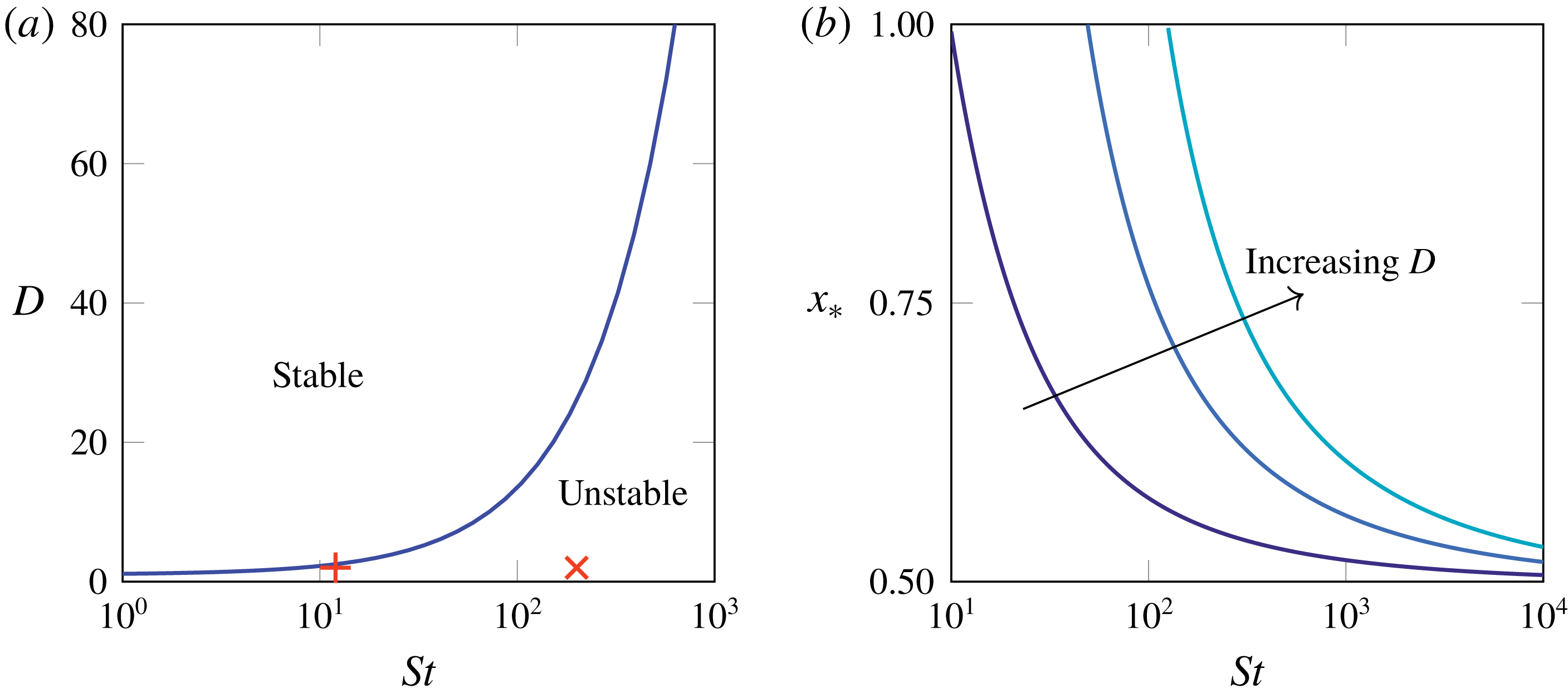
The neutral-stability curve separating regions of stability and instability is found by setting
 $c$
to zero. We show the resulting relation between the critical draw ratio and the Stokes number, namely
 $$\begin{eqnarray}St=8D\,[\tan ^{-1}\sqrt{D-1}]^{2}\end{eqnarray}$$
for
 $1\leqslant D<\infty$
, in figure 2(a). For a fixed gravitational parameter
 $St$
, (3.6) gives a critical minimum draw ratio below which the tension becomes negative in a region near the bottom of the sheet. Alternatively, for a fixed draw ratio
 $D$
, (3.6) gives a maximum value of the gravitational parameter
 $St$
above which the tension is negative near the bottom of the sheet. In either case, the size of the region in which the tension is negative increases. The value of
 $x$
at which the tension changes sign, namely
 $$\begin{eqnarray}x_{\ast }=\frac{2}{\sqrt{a}}\cos ^{-1}\sqrt{\frac{2a}{St}}\end{eqnarray}$$
is plotted versus
 $St$
for different values of
 $D$
in figure 2(b). As either
 $St$
increases or
 $D$
decreases, the length of the interval
 $(x_{\ast },1]$
in which the tension is negative increases.
We note that (3.6) represents a balance between drawing and gravity, i.e. the parameters
 $St$
and
 $D$
; inertia does not affect whether the sheet is initially stable or unstable. However, the neutral-stability curve would be different had we used a different initial thickness profile. For example, if the sheet is thicker and therefore heavier, it will stretch faster under gravity, and is more likely to be unstable. On the other hand, if the initial thickness profile were chosen to make the centreline stable at a smaller draw ratio
 $D$
than the critical value shown in figure 2(a), then the thickness and velocity profile would evolve towards (3.3) over a time scale of order
 $\unicode[STIX]{x1D716}^{-2}$
, ultimately rendering the sheet unstable to buckling. The neutral-stability curve (3.6) therefore gives an absolute lower bound on the draw ratio
 $D$
at which stable drawing can be achieved for a given value of
 $St$
.
(a) Neutral-stability curve for an initially flat sheet with uniform viscosity. The red
 $+$
and
 $\times$
denote the positions for
 $D=2$
and
 $St=12$
and
 $200$
respectively, which will be used in the solutions shown in figure 3. (b) Position
 $x_{\ast }$
at which tension in the sheet (right-hand side of (2.22)) changes sign as a function of Stokes number
 $St$
at draw ratios
 $D=2,5$
and
 $10$
.

4 Buckling solutions
4.1 Early-time behaviour
We perform a linear-stability analysis of an initially planar centreline by considering a perturbation in which
 $|H(x,t)|\ll 1$
. Linearization of (2.23) removes the dependence of
 $c$
upon
 $H$
, and therefore
 $c(t)$
remains fixed at its initial value
 $c(0)$
, given by (3.5). We decompose
 $H(x,t)$
into Fourier modes
 $\text{e}^{\unicode[STIX]{x1D706}t}\unicode[STIX]{x1D713}(x)$
, which grow if
 $\operatorname{Re}[\unicode[STIX]{x1D706}]>0$
and decay if
 $\operatorname{Re}[\unicode[STIX]{x1D706}]<0$
. Upon linearizing, the centreline evolution equation (2.24) turns into the generalized eigenvalue problem
 $$\begin{eqnarray}\unicode[STIX]{x1D706}^{2}\widehat{Re}\,h(x)\unicode[STIX]{x1D713}(x)+\frac{4\unicode[STIX]{x1D706}}{3}\left(h(x)^{3}\unicode[STIX]{x1D713}(x)^{\prime \prime }\right)^{\prime \prime }=\left[\left(St\int _{x}^{1}h(s)\,\text{d}s+c(0)\right)\unicode[STIX]{x1D713}^{\prime }(x)\right]^{\prime },\end{eqnarray}$$
with boundary conditions
 $\unicode[STIX]{x1D713}(x)=\unicode[STIX]{x1D713}^{\prime \prime }(x)=0$
at
 $x=0$
,
 $1$
, and primes denote differentiation. To enable numerical solution of (4.1), we introduce
 $\unicode[STIX]{x1D6FA}(x)=\unicode[STIX]{x1D706}\unicode[STIX]{x1D713}(x)$
to obtain a linear eigenvalue problem, where
 $\unicode[STIX]{x1D713}$
and
 $\unicode[STIX]{x1D6FA}$
are coupled, and discretize in space using second-order finite differences. The resulting matrix equation can then be solved using eig in MATLAB.
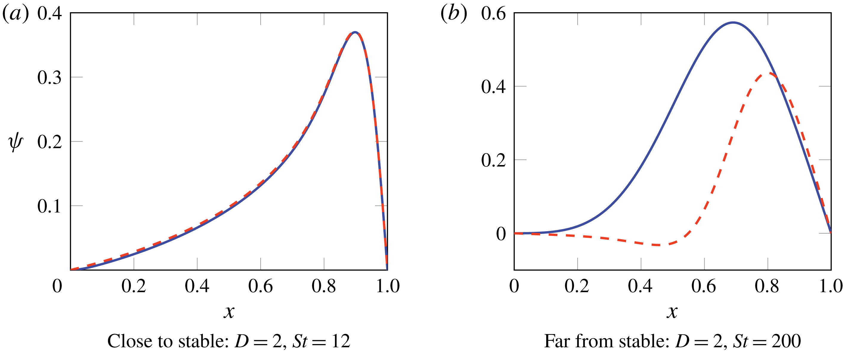
We solve the eigenvalue problem (4.1) numerically for
 $D=2$
,
 $St=12$
(marked with a red + in the
 $D$
–
 $St$
space shown in figure 2
a) and for
 $D=2$
,
 $St=200$
(red
 $\times$
in the
 $D$
–
 $St$
space shown in figure 2
a), for
 $\widehat{Re}=0$
(blue) and
 $\widehat{Re}=100$
(red, dashed). In both cases, we find that all eigenvalues are real, and we show in figure 3 the fastest-growing mode, corresponding to the largest value of
 $\unicode[STIX]{x1D706}$
. We note that
 $D=2$
,
 $St=12$
is close to the stability threshold, so we expect the growth rate to be small, while
 $D=2$
,
 $St=200$
is far from the stability boundary and we expect fast buckling.
Fastest-growing eigenmodes of (4.1) corresponding to centreline shape at early times: (a,b) correspond to the red
 $+$
and the red
 $\times$
in figure 2(a), respectively. In each case blue is for
 $\widehat{Re}=0$
and dashed red is for
 $\widehat{Re}=100$
. Corresponding growth rates are (a)
 $\unicode[STIX]{x1D706}=4.65\times 10^{-3}$
for both values of
 $\widehat{Re}$
, and (b)
 $\unicode[STIX]{x1D706}=31$
for
 $\widehat{Re}=0$
and
 $\unicode[STIX]{x1D706}=3.74$
for
 $\widehat{Re}=100$
respectively.

In the almost-stable regime (figure 3
a), the upward force at the draw rollers
 $|c(0)|\ll 1$
, and hence only a short segment of the sheet near
 $x=1$
, experiences the small compressive force that drives the buckling of the entire sheet, and the growth rate is small:
 $\unicode[STIX]{x1D706}\approx 4.65\times 10^{-3}$
for both
 $\widehat{Re}=0$
and
 $\widehat{Re}=100$
. We also observe that the rescaled Reynolds number
 $\widehat{Re}$
appears to have very little impact on the sheet dynamics: the fastest-growing eigenmodes are almost indistinguishable for
 $\widehat{Re}=0$
and
 $\widehat{Re}=100$
.
In the far-from-stable case (figure 3
b), the compressive force is larger, so a substantial portion of the almost-flat sheet experiences compression, and the growth rate is larger:
 $\unicode[STIX]{x1D706}=31$
for
 $\widehat{Re}=0$
and
 $\unicode[STIX]{x1D706}=3.74$
for
 $\widehat{Re}=100$
. The Reynolds number plays a more significant role in this regime. With the larger value of
 $\widehat{Re}$
, the fastest-growing eigenmode is more oscillatory and has a smaller growth rate; in other words, the length scale is shorter and the time scale is longer, in agreement with the scalings (2.5). For this fast-growing mode, the need to overcome inertia significantly slows the initial growth. Furthermore, a highly oscillatory centreline can accommodate the same excess length as a single buckle but with a smaller amplitude, so the fluid does not have to travel as far or as quickly. As a result, a system with larger Reynolds number exhibits more oscillatory behaviour at early times when inertia is important. These arguments also explain the role of
 $Re$
in the scalings (2.5).
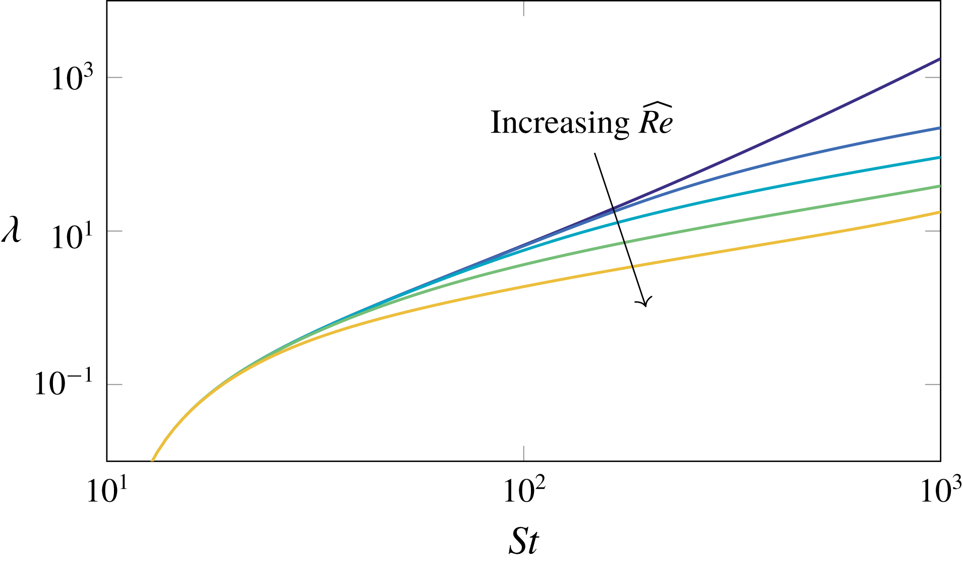
We investigate the variation of growth rate
 $\unicode[STIX]{x1D706}$
with process parameters in more detail in figure 4. We see that the growth rate increases as
 $St$
increases, and always decreases for larger
 $\widehat{Re}$
. This is as expected: increasing the effect of gravity produces a larger destabilizing compressive force over a longer section of the sheet (see figure 2
b), while inertia acts to slow down the onset of buckling.
Early-time buckling growth rates (eigenvalues of (4.1)) as a function of Stokes number
 $St$
at
 $\widehat{Re}=0,0.1,1,10$
and
 $100$
and draw ratio
 $D=2$
.

4.2 Numerical solution
To determine the full nonlinear evolution of the centreline profile, we solve the evolution equation (2.24) numerically, subject to the boundary conditions (2.21), using the method of lines, with second-order finite differencing in space. We initialize the computation at small
 $t$
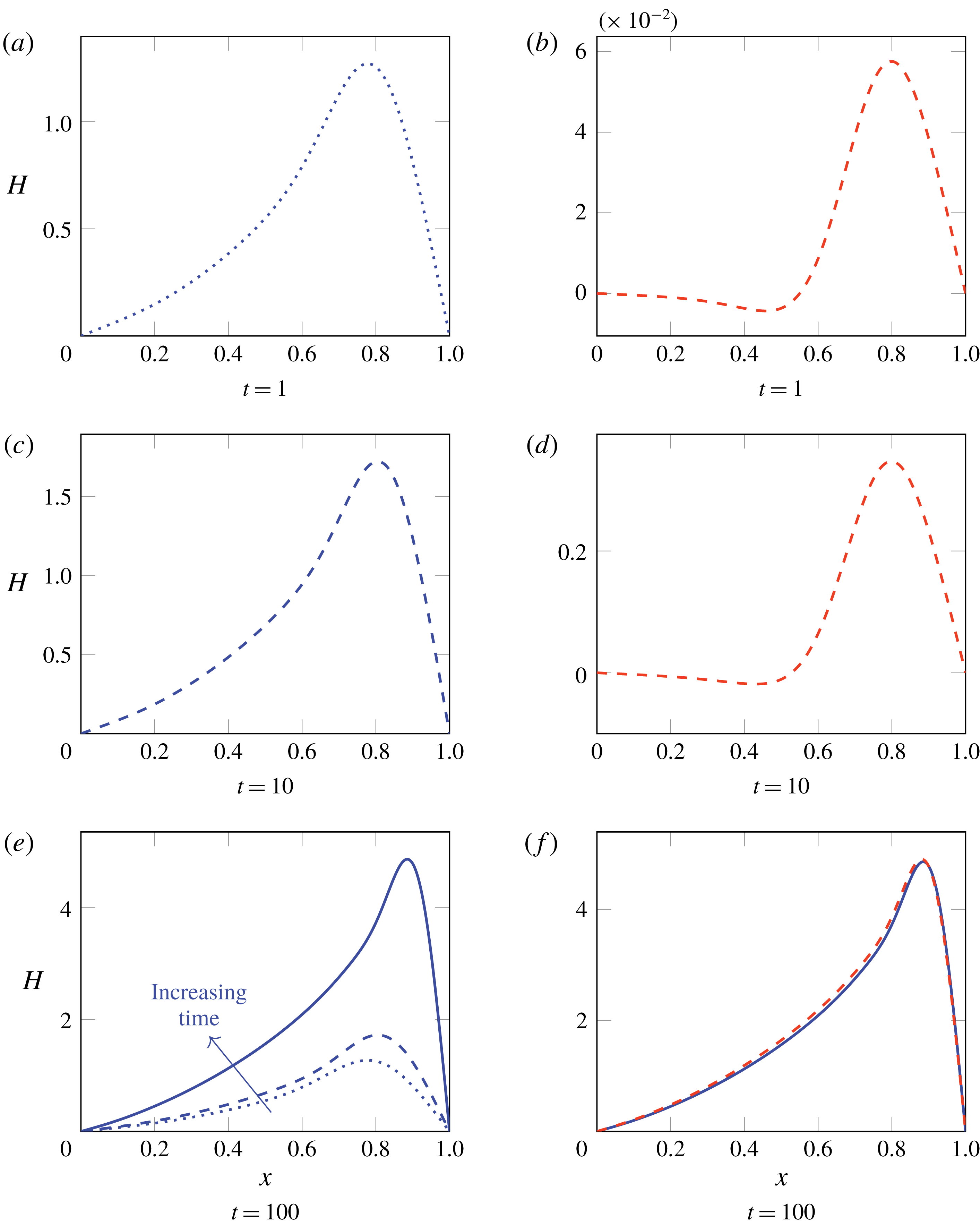
using the most unstable mode as identified in § 4.1. In figure 5, we illustrate the evolution of the sheet in time by plotting a series of snapshots of a sheet centreline with
 $D=2$
,
 $St=200$
, for both
 $\widehat{Re}=0$
and
 $\widehat{Re}=100$
.
Numerical solutions to (2.21), (2.24) with
 $D=2$
,
 $St=200$
and scaled Reynolds numbers
 $\widehat{Re}=0$
(a,c,e: blue lines) and
 $\widehat{Re}=100$
(b,d,f: dashed red lines). The solutions at
 $t=1$
and
 $t=10$
are also included in (e) for comparison, and the solution for
 $\widehat{Re}=0$
is included as a solid blue line in (f) for comparison.

We see that the early-time solutions are dramatically different for different
 $\widehat{Re}$
. At
 $t=1$
the centreline profiles still resemble the results of the linear-stability analysis shown in figure 3 (see figure 5
a,b), and the amplitude is much smaller for larger
 $\widehat{Re}$
, as expected. However, as time proceeds, solutions for different values of
 $\widehat{Re}$
become similar and, by
 $t=100$
, the profiles are virtually independent of the value of
 $\widehat{Re}$
(see figure 5
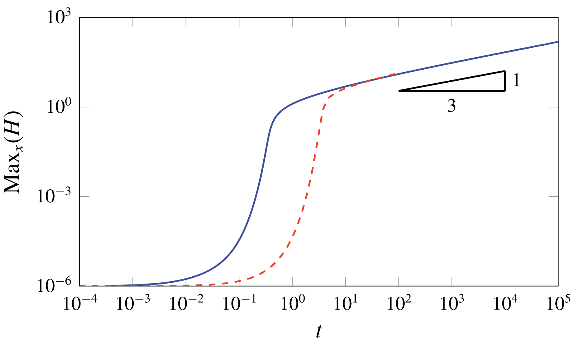
e,f). In figure 6, we further investigate the influence of inertia over short and long time scales by showing the maximum amplitude of the centreline (defined as
 $\max _{x}|H|$
) as a function of time. As suggested by the snapshots in figure 5, the amplitude depends significantly on the value of
 $\widehat{Re}$
at early times when inertia slows down buckling. However, as time increases the amplitudes for different values of
 $\widehat{Re}$
converge. We also note that the growth of the amplitude at late time appears to be close to
 $\max _{x}|H|\sim t^{1/3}$
.
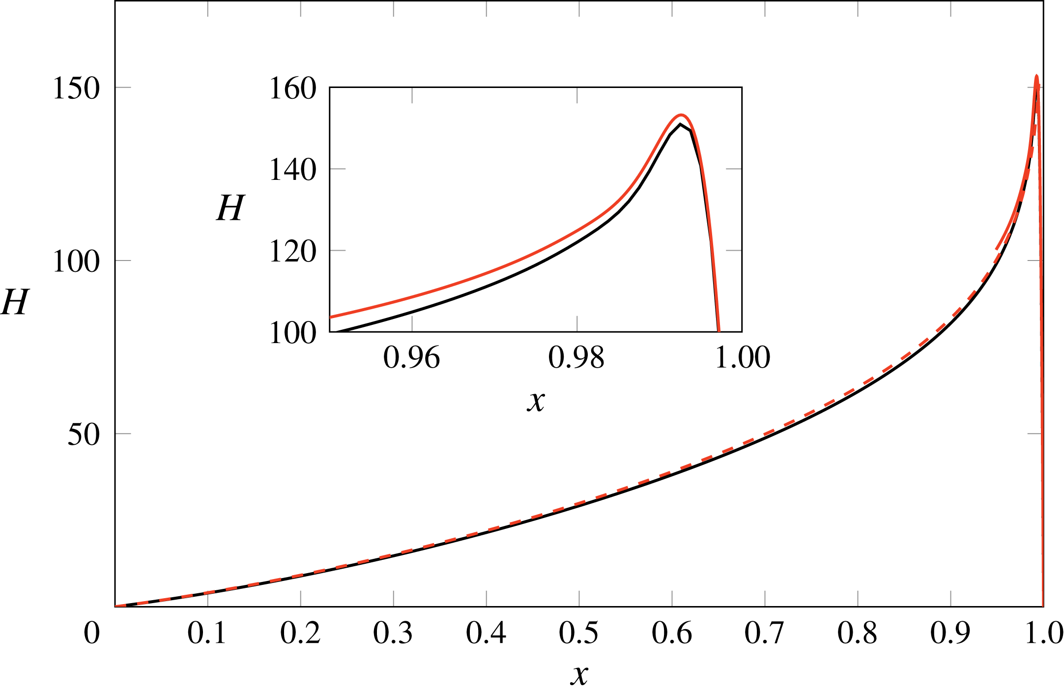
In figure 7, we show the centreline profile computed at very late time
 $t=10^{5}$
, with
 $D=2$
,
 $St=200$
and
 $\widehat{Re}=0$
. We observe that the amplitude has become very large, with a pronounced peak close to
 $x=1$
. The resulting large gradients in the region near
 $x=1$
necessitate the use of an increasingly fine grid to maintain accuracy; at
 $t=10^{5}$
, the peak is located in
 $x\in [0.99,1]$
and a mesh spacing of
 $1.25\times 10^{-3}$
gives a relative error of
 $10^{-2}$
. In the next section we develop a late-time analysis to explain and quantify both the collapse of data at late times, as demonstrated in figures 5 and 6, and the spatial localization noted in figure 7.
Log–log plot of centreline amplitude as a function of time for
 $D=2$
,
 $St=200$
,
 $\widehat{Re}=0$
(blue) and
 $\widehat{Re}=100$
(red, dashed).

Centreline shape
 $H(x,t)$
at
 $t=10^{5}$
with draw ratio
 $D=2$
, Stokes number
 $St=200$
and Reynolds number
 $\widehat{Re}=0$
. The numerical solution to (2.21), (2.24) is shown in black. The hybrid asymptotic–numerical solution described in § 5.5 is shown in red, with the dashed curve showing the outer solution (5.7) and the solid curve the inner numerical solution of (5.17).

5 Late-time analysis
5.1 Scaling analysis
Since the numerical solutions shown in figures 5 and 6 indicate that inertia does not play a role in the late-time behaviour, we neglect inertia in the analysis to follow and justify this simplification a posteriori. We therefore set
 $\widehat{Re}=0$
in equation (2.24) to obtain
 $$\begin{eqnarray}\underbrace{\left(\frac{4h^{3}}{3}H_{xxt}\right)_{xx}}_{bending}=\left[\left(\underbrace{St\int _{x}^{1}h(s)\,\text{d}s}_{gravity}+\underbrace{\vphantom{\int _{x}^{1}h(s)}c(t)}_{tension}\right)H_{x}\right]_{x},\end{eqnarray}$$
where we have identified the three labelled terms with the contributions due to bending, gravity and the force at
 $x=1$
,
 $c(t)$
. In the limit
 $t\rightarrow \infty$
, the bending term on the left-hand side of (5.1) is lower order than the right-hand side, and therefore negligible at leading order in the majority of the sheet. Since there are then two fewer spatial derivatives in the leading-order governing equations, the limit
 $t\rightarrow \infty$
is a singular perturbation, and we anticipate that there will be boundary layers near either end of the sheet where the bending term is significant. Near
 $x=0$
, the gravity term in (5.1) is
 $O(1)$
and therefore balances the bending term in a boundary layer where
 $x=O(t^{-1/2})$
. However, near
 $x=1$
, the gravity term scales with
 $1-x$
, and the bending, gravity and tension terms all balance if
 $c(t)=O(t^{-1/3})$
and
 $1-x=O(t^{-1/3})$
.
Finally, we write the governing equation (2.23) for the downstream tension
 $c(t)$
in the form
 $$\begin{eqnarray}c(t)=\frac{1}{b}\left[-m+\frac{1}{2}\frac{\text{d}}{\text{d}t}\int _{0}^{1}H_{x}(x,t)^{2}\,\text{d}x\right],\end{eqnarray}$$
where the two constants
 $$\begin{eqnarray}b=\frac{1}{4}\int _{0}^{1}\frac{\text{d}x}{h(x)},\quad m=\frac{St}{4}\int _{0}^{1}\int _{x}^{1}\frac{h(s)}{h(x)}\,\text{d}s\,\text{d}x-(D-1)\end{eqnarray}$$
are in principle both determined a priori. From § 3 we know that
 $m$
, which measures the difference between the compressive gravitational stress and the tension due to drawing, must be positive for the sheet to buckle. We identify the final term in (5.2) as the viscous tension caused by lengthening of the centreline.
We have argued above that
 $c(t)=O(t^{-1/3})\rightarrow 0$
as
 $t\rightarrow \infty$
, and therefore the two terms in square brackets in (5.2) must balance. We find that the dominant contribution to the length integral comes from the downstream boundary layer where
 $1-x=O(t^{-1/3})$
, and we then obtain a balance in (5.2) if
 $H(x,t)=O(t^{1/3})$
as
 $t\rightarrow \infty$
, in agreement with figure 6.
5.2 Governing equations in three regions
Based on the above scaling arguments, we now present the leading-order governing equations to be solved in three distinct asymptotic regions, namely the bulk of the sheet, where bending is unimportant, and the two boundary layers at either end. Since the sheet thickness
 $h(x)$
is independent of
 $t$
, in the limit as
 $t\rightarrow \infty$
in which the boundary-layer widths both shrink towards zero, the thickness inside each boundary layer becomes uniform to leading order.
In the outer region where
 $x=O(1)$
, the bending and tension terms in (5.1) are smaller than the gravity term, by factors of order
 $t^{-1}$
and
 $t^{-1/3}$
, respectively. To lowest order, the centreline profile therefore satisfies
 $$\begin{eqnarray}H_{x}\int _{x}^{1}h(s)\,\text{d}s=A(t),\end{eqnarray}$$
where
 $StA(t)$
is the tension in the sheet and, from our scaling arguments, we expect
 $A(t)=O(t^{1/3})$
as
 $t\rightarrow \infty$
.
In the top boundary layer where
 $x=O(t^{-1/2})$
, we have a balance between the bending and gravity terms, but the tension term remains negligible to leading order. Thus (5.1) reduces to
 $$\begin{eqnarray}H_{xxxxt}=\left[\frac{3St}{4h(0)^{3}}\int _{0}^{1}h(s)\,\text{d}s\right]H_{xx},\end{eqnarray}$$
in which the factor in square brackets is an a priori known constant. We integrate (5.5), subject to
 $H=H_{xxt}=0$
at
 $x=0$
and matching with (5.4), to get
 $$\begin{eqnarray}H_{xxt}-\left[\frac{3St}{4h(0)^{3}}\int _{0}^{1}h(s)\,\text{d}s\right]H=-\frac{3St}{4h(0)^{3}}\,A(t)\,x.\end{eqnarray}$$
For the solutions of (5.4) and (5.6) to match, the leading-order outer solution must satisfy
 $H(0,t)=0$
, so that the relevant solution of (5.4) is
 $$\begin{eqnarray}H(x,t)=A(t)\int _{0}^{x}\frac{\text{d}r}{\displaystyle \int _{r}^{1}h(s)\,\text{d}s}.\end{eqnarray}$$
The leading-order outer solution is thus completely determined once we have solved for the amplitude function
 $A(t)$
. It follows from (5.7) that the solution
 $H(x,t)$
of (5.6) in the upper boundary layer must be smaller than the outer solution by a factor of
 $t^{-1/2}$
: this is a weak passive boundary layer in which the curvature
 $H_{xx}$
adjusts to satisfy the zero moment condition at
 $x=0$
. For matching with the bottom boundary layer, we expand (5.7) as
 $x\rightarrow 1$
to obtain
 $$\begin{eqnarray}H(x,t)\sim A(t)\left[-\frac{1}{h(1)}\log (1-x)+C\right],\end{eqnarray}$$
where
 $C$
denotes the (known) constant
 $$\begin{eqnarray}C=\int _{0}^{1}\left(\frac{1}{\displaystyle \int _{x}^{1}h(s)\,\text{d}s}-\frac{1}{(1-x)h(1)}\right)\,\text{d}x,\end{eqnarray}$$
which quantifies the difference between the deflection in the case of uniform thickness and an arbitrary thickness profile.
Finally we consider the downstream boundary layer, where
 $1-x=O(t^{-1/3})$
and all three terms balance in (5.1) to give the leading-order equation
 $$\begin{eqnarray}\frac{4h(1)^{3}}{3}H_{xxxxt}=\left[(St\,h(1)(1-x)+c(t))H_{x}\right]_{x}.\end{eqnarray}$$
Our focus for the remainder of this section is on the solution of the inner evolution equation (5.10) subject to the relevant matching and boundary conditions. We first reduce the problem to canonical form.
5.3 Canonical boundary-layer problem
We normalize the problem in the downstream boundary layer at
 $x=1$
by scaling as follows:
 $$\begin{eqnarray}\displaystyle & \displaystyle H(x,t)=\sqrt{\frac{8m}{3St}}h(1)\,\tilde{t}^{1/3}F(\unicode[STIX]{x1D702},T), & \displaystyle\end{eqnarray}$$
 $$\begin{eqnarray}\displaystyle & \displaystyle A(t)=\sqrt{\frac{8m}{3St}}h(1)^{2}\,\tilde{t}^{1/3}\unicode[STIX]{x1D6FC}(T), & \displaystyle\end{eqnarray}$$
 $$\begin{eqnarray}\displaystyle & \displaystyle c(t)=-St\,h(1)\,\tilde{t}^{-1/3}K(T), & \displaystyle\end{eqnarray}$$
 $$\begin{eqnarray}\tilde{t}=\left(\frac{3St}{4h(1)^{2}}\right)t,\quad \unicode[STIX]{x1D702}=(1-x)\,\tilde{t}^{1/3},\quad T=h(1)C+\frac{1}{3}\log (\tilde{t}),\end{eqnarray}$$
and the form of the scalings (5.11) arises from a balance between tension, compression and gravity. The evolution equation (5.10) is transformed to
 $$\begin{eqnarray}{\textstyle \frac{1}{3}}[F_{T}+\unicode[STIX]{x1D702}F_{\unicode[STIX]{x1D702}}+F]_{\unicode[STIX]{x1D702}\unicode[STIX]{x1D702}\unicode[STIX]{x1D702}\unicode[STIX]{x1D702}}=[(\unicode[STIX]{x1D702}-K(T))F_{\unicode[STIX]{x1D702}}]_{\unicode[STIX]{x1D702}},\end{eqnarray}$$
the boundary conditions (2.21) imply that
 $$\begin{eqnarray}F=F_{\unicode[STIX]{x1D702}\unicode[STIX]{x1D702}}=0\quad \text{at }\unicode[STIX]{x1D702}=0\end{eqnarray}$$
and matching with (5.8) leads to the far-field condition
 $$\begin{eqnarray}F(\unicode[STIX]{x1D702},T)\sim \unicode[STIX]{x1D6FC}(T)(T-\log \unicode[STIX]{x1D702})\quad \text{as }\unicode[STIX]{x1D702}\rightarrow \infty .\end{eqnarray}$$
Finally, the length constraint (5.2) reduces to
 $$\begin{eqnarray}\int _{0}^{\infty }F_{\unicode[STIX]{x1D702}}(\unicode[STIX]{x1D702},T)^{2}\,\text{d}\unicode[STIX]{x1D702}\equiv 1.\end{eqnarray}$$
We have thus removed all the parameters from the boundary-layer problem, and only have to solve it once.
5.4 Asymptotic behaviour
A slight simplification is obtained by writing the problem (5.13)–(5.16) in terms of
 $G(\unicode[STIX]{x1D702},T):=F_{\unicode[STIX]{x1D702}}(\unicode[STIX]{x1D702},T)$
, which satisfies
 $$\begin{eqnarray}\displaystyle \displaystyle {\textstyle \frac{1}{3}}[G_{T}+\unicode[STIX]{x1D702}G_{\unicode[STIX]{x1D702}}+2G]_{\unicode[STIX]{x1D702}\unicode[STIX]{x1D702}}+(K(T)-\unicode[STIX]{x1D702})G & \!=\! & \displaystyle \unicode[STIX]{x1D6FC}(T),\end{eqnarray}$$
 $$\begin{eqnarray}\displaystyle \displaystyle \int _{0}^{\infty }G(\unicode[STIX]{x1D702},T)^{2}\,\text{d}\unicode[STIX]{x1D702} & = & \displaystyle 1,\end{eqnarray}$$
 $$\begin{eqnarray}\displaystyle \displaystyle G_{\unicode[STIX]{x1D702}}(\unicode[STIX]{x1D702},T) & \!=\! & \displaystyle 0\hphantom{\unicode[STIX]{x1D6FC}(T)\hspace{12.1pt}}\text{at }\unicode[STIX]{x1D702}=0,\end{eqnarray}$$
 $$\begin{eqnarray}\displaystyle \displaystyle G(\unicode[STIX]{x1D702},T) & \!\rightarrow \! & \displaystyle 0\hphantom{T\unicode[STIX]{x1D6FC}(T)\hspace{5.4pt}}\text{as }\unicode[STIX]{x1D702}\rightarrow \infty ,\end{eqnarray}$$
 $$\begin{eqnarray}\displaystyle \displaystyle \int _{0}^{\unicode[STIX]{x1D702}}G\left(\unicode[STIX]{x1D702}^{\prime },T\right)\,\text{d}\unicode[STIX]{x1D702}^{\prime }+\unicode[STIX]{x1D6FC}(T)\log \unicode[STIX]{x1D702} & \!\rightarrow \! & \displaystyle T\unicode[STIX]{x1D6FC}(T)\quad \text{as }\unicode[STIX]{x1D702}\rightarrow \infty .\end{eqnarray}$$
We recall from (5.12) that the surrogate time variable
 $T$
scales with
 $\log t$
as
 $t\rightarrow \infty$
. We would hope that the problem (5.17) admits a limiting solution in which
 $G(\unicode[STIX]{x1D702},T)$
becomes independent of
 $T$
and thus the local behaviour becomes self-similar. However, here the convergence to self-similarity is very slow, as a consequence of the appearance of
 $T$
on the right-hand side of (5.17e
), which originates from the logarithmic matching condition (5.8). Indeed, we find that the large-
 $T$
behaviour of the solution of (5.17) involves a full logarithmic expansion of the form
 $$\begin{eqnarray}\left.\begin{array}{@{}c@{}}\displaystyle G(\unicode[STIX]{x1D702},T)\sim G_{0}(\unicode[STIX]{x1D702})+\frac{G_{1}(\unicode[STIX]{x1D702})}{T}+\cdots \,,\quad \unicode[STIX]{x1D6FC}(T)\sim \frac{\unicode[STIX]{x1D6FC}_{1}}{T}+\frac{\unicode[STIX]{x1D6FC}_{2}}{T^{2}}+\cdots \,,\\ \displaystyle K(T)\sim K_{0}+\frac{K_{1}}{T}+\cdots \end{array}\right\}\quad \text{as }T\rightarrow \infty .\end{eqnarray}$$
At leading order, we find that
 $G_{0}$
satisfies the boundary-value problem
 $$\begin{eqnarray}\displaystyle & \displaystyle \unicode[STIX]{x1D702}G_{0}^{\prime \prime \prime }(\unicode[STIX]{x1D702})+4G_{0}^{\prime \prime }(\unicode[STIX]{x1D702})+3(K_{0}-\unicode[STIX]{x1D702})G_{0}(\unicode[STIX]{x1D702})=0, & \displaystyle\end{eqnarray}$$
 $$\begin{eqnarray}\displaystyle & \displaystyle G_{0}^{\prime }(0)=0,\quad G_{0}(\unicode[STIX]{x1D702})\rightarrow 0\quad \text{as }\unicode[STIX]{x1D702}\rightarrow \infty . & \displaystyle\end{eqnarray}$$
Equation (5.19a
) is singular at
 $\unicode[STIX]{x1D702}=0$
, as a result of which the first boundary condition in (5.19b
) actually removes two degrees of freedom for the solution for
 $G_{0}$
. This eigenvalue problem (5.19) admits non-trivial solutions for
 $G_{0}$
only if
 $K_{0}$
takes one of a discrete set of positive values, and the amplitude of
 $G_{0}$
is then fixed using (5.17b
), i.e.
 $$\begin{eqnarray}\int _{0}^{\infty }G_{0}(\unicode[STIX]{x1D702})^{2}\,\text{d}\unicode[STIX]{x1D702}=1.\end{eqnarray}$$
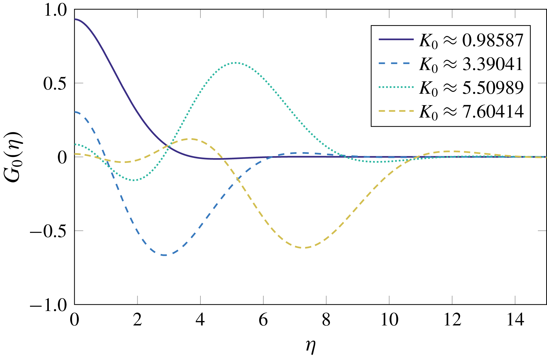
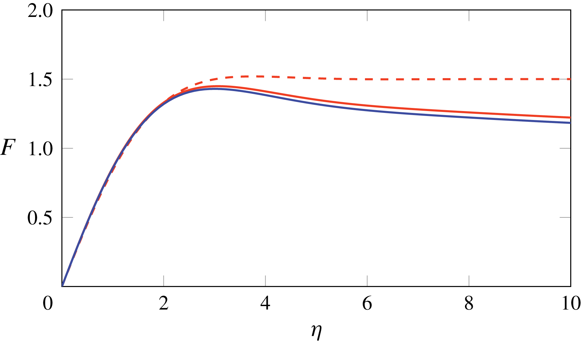
The resulting eigenfunctions corresponding to the first four eigenvalues are plotted in figure 8. Evidently the higher modes become increasingly oscillatory, and we hypothesize that only the lowest mode, with
 $K_{0}\approx 0.986$
, is physically relevant. We then read off the first approximation for
 $\unicode[STIX]{x1D6FC}$
from (5.17e
), i.e.
 $$\begin{eqnarray}\unicode[STIX]{x1D6FC}_{1}=\int _{0}^{\infty }G_{0}(\unicode[STIX]{x1D702})\,\text{d}\unicode[STIX]{x1D702}\approx 1.5.\end{eqnarray}$$
Since
 $T$
scales with
 $\log (t^{1/3})$
, we calculate one further term in the large-
 $T$
expansion for improved accuracy at moderately large values of
 $t$
. We shall see below that it is helpful to solve the adjoint version of (5.19), namely
 $$\begin{eqnarray}\displaystyle & \displaystyle \unicode[STIX]{x1D702}\unicode[STIX]{x1D719}^{\prime \prime \prime }(\unicode[STIX]{x1D702})-\unicode[STIX]{x1D719}^{\prime \prime }(\unicode[STIX]{x1D702})-3(K_{0}-\unicode[STIX]{x1D702})\unicode[STIX]{x1D719}(\unicode[STIX]{x1D702})=0, & \displaystyle\end{eqnarray}$$
 $$\begin{eqnarray}\displaystyle & \displaystyle \unicode[STIX]{x1D719}^{\prime }(0)=0,\quad \unicode[STIX]{x1D719}(\unicode[STIX]{x1D702})\rightarrow 0\quad \text{as }\unicode[STIX]{x1D702}\rightarrow \infty , & \displaystyle\end{eqnarray}$$
 $\unicode[STIX]{x1D719}(\unicode[STIX]{x1D702})$
when
 $K_{0}$
is equal to one of the eigenvalues identified above, and we again take the smallest.
The eigenfunctions corresponding to the four smallest eigenvalues
 $K_{0}$
of the problem (5.19).

At
 $O(T^{-1})$
we find that
 $G_{1}$
satisfies the boundary-value problem
 $$\begin{eqnarray}\displaystyle & \displaystyle \unicode[STIX]{x1D702}G_{1}^{\prime \prime \prime }(\unicode[STIX]{x1D702})+4G_{1}^{\prime \prime }(\unicode[STIX]{x1D702})+3(K_{0}-\unicode[STIX]{x1D702})G_{1}(\unicode[STIX]{x1D702})=3(\unicode[STIX]{x1D6FC}_{1}-K_{1}G_{0}(\unicode[STIX]{x1D702})), & \displaystyle\end{eqnarray}$$
 $$\begin{eqnarray}\displaystyle & \displaystyle G_{1}^{\prime }(0)=0,\quad G_{1}(\unicode[STIX]{x1D702})\rightarrow 0\quad \text{as }\unicode[STIX]{x1D702}\rightarrow \infty , & \displaystyle\end{eqnarray}$$
as well as the normalization condition
 $$\begin{eqnarray}\int _{0}^{\infty }G_{0}(\unicode[STIX]{x1D702})G_{1}(\unicode[STIX]{x1D702})\,\text{d}\unicode[STIX]{x1D702}=0.\end{eqnarray}$$
Since the value of
 $K_{0}$
is chosen such that (5.19) admits non-trivial solutions, (5.22) has no solutions unless the inhomogeneous right-hand side is orthogonal to the solution
 $\unicode[STIX]{x1D719}$
of the adjoint problem (5.22). This solvability condition determines the first correction to
 $K$
, namely
 $$\begin{eqnarray}K_{1}=\left.\unicode[STIX]{x1D6FC}_{1}\int _{0}^{\infty }\unicode[STIX]{x1D719}(\unicode[STIX]{x1D702})\,\text{d}\unicode[STIX]{x1D702}\right/\int _{0}^{\infty }G_{0}(\unicode[STIX]{x1D702})\unicode[STIX]{x1D719}(\unicode[STIX]{x1D702})\,\text{d}\unicode[STIX]{x1D702}\approx 2.2,\end{eqnarray}$$
where we have used both
 $G_{0}$
and the solution
 $\unicode[STIX]{x1D719}$
to the adjoint problem (5.21). With
 $K_{1}$
defined by (5.23), we can solve (5.22) for
 $G_{1}(\unicode[STIX]{x1D702})$
, with the amplitude of the complementary function determined by (5.22c
). We then obtain the next correction to
 $\unicode[STIX]{x1D6FC}$
from (5.17e
), i.e.
 $$\begin{eqnarray}\unicode[STIX]{x1D6FC}_{2}=\int _{0}^{\infty }\left(G_{1}(\unicode[STIX]{x1D702})+\frac{\unicode[STIX]{x1D6FC}_{1}}{1+\unicode[STIX]{x1D702}}\right)\,\text{d}\unicode[STIX]{x1D702}\approx 0.5146.\end{eqnarray}$$
We obtain the late-time solution for the centreline profile as an asymptotic expansion of the form
 $$\begin{eqnarray}F(\unicode[STIX]{x1D702},T)\sim F_{0}(\unicode[STIX]{x1D702})+T^{-1}F_{1}(\unicode[STIX]{x1D702})+\cdots \quad \text{as }T\rightarrow \infty\end{eqnarray}$$
by integrating
 $G_{0}(\unicode[STIX]{x1D702})$
and
 $G_{1}(\unicode[STIX]{x1D702})$
with respect to
 $\unicode[STIX]{x1D702}$
. The resulting leading-order and first-order approximations to
 $F(\unicode[STIX]{x1D702})$
are shown in figure 9 using red dashed and red solid curves respectively, with
 $T=10$
. The
 $O(T^{-1})$
correction does not make a noticeable difference close to
 $\unicode[STIX]{x1D702}=0$
, but becomes increasingly important as
 $\unicode[STIX]{x1D702}$
increases. The leading-order approximation
 $F_{0}(\unicode[STIX]{x1D702})$
tends to a constant as
 $\unicode[STIX]{x1D702}\rightarrow \infty$
, so we need to include the first correction to get the correct logarithmic behaviour (5.15).
Late-time solutions for the centreline shape in the lower boundary layer computed with
 $T=10$
: leading-order solution
 $F_{0}(\unicode[STIX]{x1D702})$
(red dashed); first-order approximation
 $F_{0}(\unicode[STIX]{x1D702})+T^{-1}F_{1}(\unicode[STIX]{x1D702})$
(red solid); numerical hybrid solution (blue solid).

Our analysis also determines the asymptotic behaviour of the amplitude
 $A$
of the outer solution, namely
 $$\begin{eqnarray}A\sim \sqrt{\frac{8m}{3St}}\,h(1)^{2}\,\frac{\tilde{t}^{1/3}}{T}\left(\unicode[STIX]{x1D6FC}_{1}+\frac{\unicode[STIX]{x1D6FC}_{2}}{T}+\cdots \,\right),\end{eqnarray}$$
with
 $\unicode[STIX]{x1D6FC}_{1}$
and
 $\unicode[STIX]{x1D6FC}_{2}$
the numerically determined constants given above. However, we recall from (5.12) that
 $T$
scales with
 $\log (t^{1/3})$
, and so huge values of
 $t$
correspond to moderate values of
 $T$
, (e.g. up to
 $t=10^{13}$
for the value
 $T=10$
used in figure 9). To capture the behaviour over long but realistic time scales where the large
 $T$
asymptotics do not hold, we next consider the full numerical solution of the inner problem (5.17).
5.5 Hybrid asymptotic–numerical solution
A hybrid asymptotic–numerical scheme for a perturbed eigenvalue problem with logarithmic gauge functions was developed by Ward, Heshaw & Keller (Reference Ward, Heshaw and Keller1993) and adapted by Kropinski, Ward & Keller (Reference Kropinski, Ward and Keller1995) for the case of low-Reynolds-number flow past a cylindrical body. In this scheme, rather than calculating individual terms in the logarithmic expansion separately, the entire series is calculated in one go as the function of a new variable which is the logarithm of the small parameter in the asymptotic expansion. We adopt an analogous approach here by solving the problem (5.17) numerically, treating
 $T$
as a time-like independent variable, to obtain a solution that incorporates all of the logarithmic corrections and is thus accurate up to
 $O(t^{-1/3})$
. Although this means we still have to solve a partial differential equation to determine the shape of the centreline, the rescaling into the bottom inner region means the boundary-layer problem (5.17) does not suffer from the stiffness of the original problem (2.21), (2.24), which allows for much faster computation at late times. Furthermore, we have removed any dependence on the process parameters, meaning that this boundary-layer problem must only be solved once, and the centreline shape and the force in the boundary layer may then be deduced for any process by appropriate rescalings.
Integrating (5.17a
) with respect to
 $\unicode[STIX]{x1D702}$
and imposing (5.17c
), (5.17d
) and (5.17e
) reveals the identity
 $$\begin{eqnarray}\int _{0}^{\infty }\left[\unicode[STIX]{x1D6FC}(T)+\unicode[STIX]{x1D702}G(\unicode[STIX]{x1D702},T)+\frac{\unicode[STIX]{x1D6FC}(T)K(T)}{1+\unicode[STIX]{x1D702}}\right]\,\text{d}\unicode[STIX]{x1D702}\equiv 0,\end{eqnarray}$$
which allows the force
 $K$
to be expressed in terms of
 $G$
and
 $\unicode[STIX]{x1D6FC}$
. The evolution of
 $G$
and
 $\unicode[STIX]{x1D6FC}$
is then fully determined by the differential equation (5.17a
), the boundary conditions (5.17c
), (5.17d
) and the constraint (5.17b
), together with a suitable initial guess, which does not affect the late-time behaviour. We discretize the problem (5.17) using second-order finite differencing in
 $\unicode[STIX]{x1D702}$
to give a system of ordinary differential equations in
 $T$
supplemented by two algebraic conditions. We solve this system of equations using MATLAB’s built-in differential-algebraic-equation solver
ode15i.
The resulting numerical solution for the normalized centreline profile
 $F(\unicode[STIX]{x1D702},T)$
in the boundary layer, evaluated at
 $T=10$
, is shown as the solid blue curve in figure 9. We observe that successive approximations in the large-
 $T$
expansion indeed converge towards the computed solution. The solid red curve in figure 7 shows the boundary-layer solution compared with the numerical solution of the full problem (2.21), (2.24) at
 $t=10^{5}$
, here corresponding to
 $T\approx 7.957$
. The dashed red curve shows the corresponding leading-order outer solution (5.7), with
 $A(t)$
given by (5.11b
) and
 $\unicode[STIX]{x1D6FC}(T)$
obtained from the boundary-layer solution. We observe that both the shape and the amplitude are very well captured by the hybrid computation. We also note that a high-resolution numerical solution is difficult to obtain at this late time due to the localization of bending near
 $x=1$
, an issue from which our asymptotic solution does not suffer.
5.6 Validity of late-time analysis
We conclude by examining the validity of the asymptotic assumptions made in our analysis. By reversing the normalization (5.11), (5.12), we determine how the neglected terms in the governing equations scale with
 $t$
and with the other key parameters in the problem, in particular
 $St$
, which measures the importance of gravity, and
 $m$
, which measures the excess compressive stress at
 $x=1$
. Our late-time analysis is valid when
 $\tilde{t}\gg 1$
, which corresponds to
 $t\gg D^{-2}St^{-1}$
; by using large values of
 $St$
, we are able to clearly observe the limiting behaviour at relatively manageable values of
 $t$
.
First, we recall that we assume inertia to be negligible throughout. We can readily calculate the size of the neglected inertia term in each of the three regions considered. We find that it is largest in the lower boundary layer, where it is smaller than the retained terms in (5.10) by a factor of order
 $(\widehat{Re}\,St)D^{-2/3}(St\,t)^{-7/3}$
. Thus, although inertia is formally negligible in the limit as
 $(St\,t)\rightarrow \infty$
, it might take a long time to become insignificant in cases where
 $\widehat{Re}\,St$
is large.
Finally we return to the question of the validity of our basic model (2.19), which breaks down whenever the dimensionless curvature
 $H_{xx}$
becomes of order
 $\unicode[STIX]{x1D716}^{-1}$
. As above, we can estimate the size of the curvature in each of the asymptotic regions identified, and we again find that it is greatest in the lower boundary layer, where
 $H_{xx}$
scales with
 $\sqrt{m\,St}\,D\,t$
. Thus geometrical nonlinearity remains unimportant as long as
 $t\ll D^{-1}m^{-1/2}St^{-1/2}\unicode[STIX]{x1D716}^{-1}$
. In particular, the curvature remains small for longer when
 $m$
is small, in other words when the excess force due to gravity and hence the rate of elongation of the sheet are small.
Collecting together the above estimates, we conclude that the late-time analysis is valid for time scales satisfying
 $$\begin{eqnarray}\left.\begin{array}{@{}c@{}}\displaystyle D^{-2}\\ \displaystyle D^{-2/7}(\widehat{Re}\,St)^{3/7}\end{array}\right\}\ll St\,t\ll \frac{1}{\unicode[STIX]{x1D716}}\frac{1}{D}\sqrt{\frac{St}{m}}.\end{eqnarray}$$
Such a region of validity exists for sufficiently small
 $\unicode[STIX]{x1D716}$
and
 $\widehat{Re}$
that
 $\unicode[STIX]{x1D716}\ll D\sqrt{St/m}$
and
 $\unicode[STIX]{x1D716}^{7/3}\widehat{Re}\ll St^{1/6}m^{-7/6}D^{-5/3}$
.
6 Discussion
In this paper we derive and analyse a model governing the thickness, velocity and centreline of a two-dimensional thin viscous sheet undergoing redraw, focusing on the distinguished limit where the Reynolds number
 $Re=O(\unicode[STIX]{x1D716}^{4})$
, where
 $\unicode[STIX]{x1D716}$
is the (small) aspect ratio of the sheet. The tension in the sheet is determined by a balance between the pulling force provided by draw rollers and the compressional force due to gravity. If gravity is sufficiently strong, then a region near the bottom of the heater zone experiences compression, causing the sheet to buckle.
We analyse sheet buckling using both linear-stability analysis and full numerical solutions. At the instability threshold, a small compressive force appears near the bottom of the sheet, and the sheet begins to buckle. Moving further from the threshold, the size of the region under compression and the magnitude of the compressive force both increase, thus modifying the centreline shape and increasing the growth rate. The buckling growth rate and length scale are also affected by the inertia of the sheet, as we explain using physical arguments. However, as the centreline continues to deform, its shape ultimately becomes independent of the Reynolds number and exhibits a single bump with its peak near the bottom of the sheet. We note that our ‘nearly planar’ model does not predict the sagging behaviour one might expect at extremely late times, when the weight of glass at the apex of the deformed sheet is large enough to pull it down past the draw rollers. Nonetheless, our results give useful insight into the initial buckling behaviour, and would provide the initial conditions for a geometrically nonlinear model that describes the subsequent evolution when the dimensionless curvature is no longer small.
Initially, while the centreline deflection remains small, the stress in the sheet is unaffected by the buckling behaviour, but at later times they are strongly coupled. Indeed, our analysis of the late-time behaviour demonstrates that the sheet centreline deforms in such a way as to expel any compression from the system: as the sheet buckles, the size of the region under compression and the magnitude of the compressive force both shrink. The bulk of the sheet is thus under tension, and the dynamics is driven by the small boundary layer at the bottom where the sheet is under compression. Matching between these regions reveals that the appropriate asymptotic expansion for large values of time
 $t$
is a double series in powers of
 $t^{1/3}$
and
 $\log (t^{1/3})$
. We circumvent the logarithmic expansion by neglecting all algebraically small corrections but retaining
 $\log (t^{1/3})$
(suitably normalized) as a dependent variable, and solving the resulting partial differential equation numerically. This hybrid asymptotic–numerical scheme yields universal predictions for the late-time behaviour which give excellent agreement with numerical solution of the full problem.
It has been established (see e.g. Filippov & Zheng Reference Filippov and Zheng2010) that sinuous centreline instability in glass sheet redraw is associated with the occurrence of compressive regions in the sheet. In three-dimensional redraw, such compressive zones always appear (even in the absence of gravity), as the sheet necks in in the transverse direction. Srinivasan et al. (Reference Srinivasan, Wei and Mahadevan2017) and O’Kiely (Reference O’Kiely2018) both perform linear-stability analysis of a such a sheet to predict where the sheet is under compression and thus where wrinkles are expected to appear. The compressive zones computed by Srinivasan et al. (Reference Srinivasan, Wei and Mahadevan2017) and O’Kiely (Reference O’Kiely2018) do not extend to the bottom of the sheet, although in practice undesirable wrinkles may be present in the final product. Thus, although the linear theory determines where buckling is likely to start, it does not tell us how the resulting wrinkles subsequently evolve or, in particular, whether they become frozen into the sheet as it exits the heater zone.
In the linearized models, the stress in the sheet is calculated in advance, and remains unaffected by any resulting evolution of the centreline. However, when the centreline is unstable, the transverse deflection must grow exponentially and, once it is the same order as the sheet thickness, start to influence the stress. Our toy two-dimensional model for redraw, which explicitly includes the mutual coupling between the tension in the sheet and the centreline evolution, provides insight into weakly nonlinear viscous buckling more generally.
Acknowledgements
D.O.K. is grateful for funding from Schott AG and the Mathematical Institute, Oxford. I.M.G. gratefully acknowledges support from the Royal Society through a Royal Society University Research Fellowship.