4.1 The OPM approach

As has been noted, the MLE of y _i,t = αy _i,t−1 + βx _i,t + η _i + ε _i,t when T is small leads to an incidental parameters problem. Lancaster (Reference Lancaster2002) suggests a solution. We are not interested in the incidental parameters η _i. We are interested in estimates of the common parameters: α and β (used to calculate the LREs and SREs of x _i,t) and σ ². We seek a reparameterization of the incidental parameters so that the incidental and common parameters are information orthogonal. To understand what reparameterization means, let us start with a simple example. If we have the following static model:

(7)$$y_{i, t} = \beta_0 + \beta_1 x_{i, t} + \eta_{i} + \epsilon_{i, t}$$

we can define a new set of incidental parameters as a function of the original incidental parameters and β ₀: $\tilde {\eta }_{i} = \eta _{i} + \beta _0$

Our static model, expressed in terms of the new incidental parameters is:

$$y_{i, t} = \tilde{\eta}_{i} + \beta_1 x_{i, t} + \epsilon_{i, t}$$

Note that although the incidental parameters have changed and their interpretation differs, the common parameters have not changed and their interpretation remains the same.

The orthogonal reparameterization proposed by Lancaster (Reference Lancaster2002) is much more complex but like the above transformation, it changes the meaning of the parameters representing the individual effects but not the meaning of the other parameters. Unlike the above, the Lancaster reparameterization also allows us to write a likelihood in which the incidental parameters are informationally orthogonal from the other parameters. To break this concept down, we begin with the concept of orthogonality.

For Equation 3, we denote the likelihood function for the data for a single case as ℓ_i(η _i,  α,  β,  σ ²). Following Lancaster (Reference Lancaster2002), suppose the incidental parameters can be reparameterized so that the likelihood function factors as:

(8)$$\ell_i( \eta_{i},\; \alpha,\; \beta,\; \sigma^2) = \ell_{i1}( \eta_{i}) \ell_{i2}( \alpha,\; \beta,\; \sigma^2) $$

where ℓ_i1 and ℓ_i2 are themselves likelihood functions. If the parameters (η _i) and (α,  β,  σ ²) are also variation independent, they are orthogonal.Footnote ¹⁸ It can then be shown that the application of maximum likelihood to the product of the ℓ_i2 for all cases produces consistent estimates of (α,  β,  σ ²) as N → ∞ when T ≥ 3 (Lancaster, Reference Lancaster2002). Lancaster (Reference Lancaster2002) provides the Poisson count model as an example of where this is possible. The likelihood of case i is:

(9)$$\ell_i( \eta_{i},\; \theta) \propto {\rm e}^{-\eta_{i}\sum_{t}{} {\exp}( x_{i, t}\theta) } \eta_{i}^{\sum_{t}{} y_{i, t}} {\rm e}^{\theta_{i}'\sum_{t}{} y_{i, t}x_{i, t}}$$

If we define $\tilde {\eta }_{i} = \eta _{i} \sum _{t}{} {\rm e}^{\theta _{i}'x_{i, t}}$, we can rewrite Equation 10 as:

(10)$$\ell_i( \tilde{\eta}_{i},\; \theta) \propto {\rm e}^{-\tilde{\eta}_{i}}\tilde{\eta}_{i}^{\sum_{t}{} y_{i, t}} \times {{\rm e}^{\theta_{i}'\sum_{t}{} y_{i, t}x_{i, t}}\over ( \sum_{t}{{\rm e}^{\theta_{i}' x_{i, t}}}) ^{\sum_{t}{}y_{i, t}}}$$

This is an orthogonal reparameterization with respect to the incidental parameters because it expresses the original likelihood as the product of two likelihoods, the first of which, $\ell _{i1} = {\rm e}^{-\tilde {\eta }_{i}}\tilde {\eta }_{i}^{\sum _{t}{} y_{i, t}}$, contains only the reparameterized incidental parameters and the second, $\ell _{i2} = {{\rm e}^{\theta _{i}'\sum _{t}{} y_{i, t}x_{i, t}}}/{( {\rm e}^{\theta _{i}'\sum _{t}{} x_{i, t}}) ^{\sum _{t}{}y_{i, t}}}$, only contains the common parameter θ Lancaster (Reference Lancaster2002).

Unfortunately, not all likelihoods can be transformed so that the incidental parameters are completely orthogonal. However, it may still be possible to reparameterize the incidental parameters so that they are information orthogonal. Informally, information orthogonality means no information about the values of the $\tilde {\eta }_{i}$ tell us anything about the values of the common parameters. Formally, if the incidental parameters are completely orthogonal as above, the following is true:

(11)$${\partial^2{\cal L}_i\over \partial\tilde{\eta}_{i}\partial\theta} = 0$$

where ${\cal L}_i$ is the log of the likelihood for the data for case i. Information orthogonality is a weaker form of orthogonality where the above is true in expectations (Lancaster, Reference Lancaster2002):

(12)$$E\left({\partial^2{\cal L}_i\over \partial\tilde{\eta}_{i}\partial\theta}\right) = 0$$

This can be interpreted as meaning that the gradient (slope) of the log likelihood with respect to the $\tilde {\eta }_{i}$ is independent of the gradient of the log likelihood with respect to the common parameter θ.Footnote ¹⁹

The purpose of seeking a reparameterization that results in information orthogonality is that it means we can place priors on the parameters and integrate out the fixed-effects. This gives us the marginal posterior for the remaining parameters and we can use Monte Carlo methods to sample values from the marginal posterior to produce estimates and credible intervals for the parameters. The estimates are consistent as N → ∞. The approach relies on the Bayesian idea of integrating out the $\tilde {\eta }_{i}$ to give us the marginal posterior distribution for the remaining parameters—although, this has many similarities to the frequentist idea of a conditional likelihood (Cox and Reid, Reference Cox and Reid1987; Lancaster, Reference Lancaster2000). Note that the orthogonal-reparameterization is not necessary in order to place a prior on and integrate out the incidental parameters but the orthogonalization means that the marginal posterior produced by integrating out the incidental parameters does not depend on the choice of prior that we place on them. In other words: we do not require any information about the individual effects.

If we wish to estimate Equation 3, an orthogonal re-parameterization of the fixed-effects, placement of priors on α, β, σ ², and the $\tilde {\eta }_{i}$, and integrating out the reparameterized fixed-effects results in the following posterior density function (Lancaster, Reference Lancaster2002):

(13)$$\eqalign{& p( \alpha,\; \beta,\; \sigma^2\vert \rm {data}) \propto( \sigma^{-{\it N}( {\it T}-1) }) \cr & \times{\exp}\left({\it {N}\over {\it T}}\sum_{t = 1}^{{\it T}-1}{{\it T}-t\over t}\alpha^t - {1\over 2\sigma^2}\sum_{t = 1}^{{\it T}-1}( y_{i, t} - \alpha y_{i, t-1}-\beta x_{i, t}) H ( y_{i, t} - \alpha y_{i, t-1}-\beta x_{i, t}) \right)\cr & \times \pi( \alpha,\; \beta,\; \sigma^2) }$$

H is defined as an operator that subtracts the mean. π(α,  β,  σ ²) represents independent, flat priors on each of the parameters, except α for which we use a uniform (− 1, 1) prior. Monte Carlo methods can be used to draw sample values of the parameters from this density distribution and the sampled values can be used to produce point estimates and credible intervals (Appendix D provides details). This approach provides a method of estimating the LRE that differs from other estimators. Instead of dividing the point estimates for β by one minus the point estimate for α, the LRE can be calculated for each pair of sampled β and α values, and the distribution of these LREs used to provide the LRE point estimate and credible interval. Pickup et al. (Reference Pickup, Gustafson, Cubranic and Evans2017) describes the mechanics of using our R package for this estimator.

4.2 The QML approach

Although the MLE of model Equation 3 with a fixed T leads to an incidental parameters problem, one can apply MLE to the first difference version of the model, as used in the GMM estimator Equation 6. Following Hsiao et al. (Reference Hsiao, Pesaran and Tahmiscioglu2002), to derive the likelihood for Equation 6, we begin by writing the joint density of Δy _i,t given Δx _i,t as:

$$\eqalign{P( \Delta y_{i, t = 1\colon T} \vert \Delta x_{i, t = 1\colon T} ) =\; & P( \Delta y_{i, T} \vert \Delta y_{i, t = 1\colon T-1},\; \Delta x_{i, t = 1\colon T} ) \cdots P( \Delta y_{i, 2} \vert \Delta y_{i, 1},\; \Delta x_{i, t = 1\colon T}) \cr & \!\!\!\times P( \Delta y_{i, 1} \vert \Delta x_{i, t = 1\colon T} ) }$$

However, the density function is not defined for Δy _i,1 because y _i,0 is unobserved. Making no assumptions about the distribution of y _i,0 and treating these as free parameters to be estimated, reintroduces the incidental parameters problem. There are as many of these free parameters as there are cases. To avoid this problem, it is necessary to assume a functional form for the distribution of Δy _i,1. Hsiao et al. (Reference Hsiao, Pesaran and Tahmiscioglu2002) propose the following feasible representation:

(14)$$\Delta y_{i, 1} = b + \sum_{s = 1}^{T} ( \Delta x_{i, s}'\pi_s) + \nu_{i, 1}$$

where b is a parameter to be estimated and π _s is a T × 1 vector of parameters to be estimated. The derivation of this representation makes assumptions about the covariates (e.g., x _i,t). It is assumed they are trend—or first difference—stationary, and weakly exogenous. Violations of either assumption will cause biased estimates. Violations of the stationarity assumption can be addressed through variable transformations but endogeneity is an assumption about the DGP. The unmodelled part of y _i,t can be a function of current and past values of x _i,t but not future values. Hsiao et al. (Reference Hsiao, Pesaran and Tahmiscioglu2002) provide the log-likelihood function based on Equations 6 and 14, which can be maximized iteratively (Kripfganz, Reference Kripfganz2016).Footnote ²⁰ Because of the iterative nature of this estimator, convergence on a solution is not guaranteed. This problem does not occur for the OPM approach, as a closed form expression of the posterior is available and so we do not need to use an iterative procedure to obtain estimates. It is also the case that the dimension of π _s increases with T, resulting in additional parameters to be estimated. There is no equivalent set of parameters for OPM, meaning it may be more efficient than QML-FE as T increases.

4.3 Trade-off between GMM and likelihood-based estimators

GMM is efficient to the extent that valid moment conditions are included and the optimal weighting matrix can be estimated. However, not all moment conditions may be known to the researcher (Kiviet et al., Reference Kiviet, Pleus and Poldermans2017), and estimating the weighting matrix can be computationally difficult. Likelihood-based estimators contain all the information regarding moment conditions in the assumptions made regarding the distribution of the data when constructing the likelihood. Therefore, likelihood-based estimators have an advantage with regards to smaller random errors and smaller confidence intervals/standard errors. A disadvantage of likelihood-based estimators is that if the distributional assumptions are incorrect, the estimator may not be consistent. With GMM estimators, the distributional assumptions are only as strict as the moment conditions included. GMM estimators, as they are applied to panel data, relax assumptions about the distribution by trading off greater random errors, particularly when T and/or N is very small. The value of the trade-off, one way or the other, is unclear as the robustness of the OPM and QML-FE estimators to violations of distributional assumptions is unknown. Their finite sample properties are only partially known and it is unknown how well they perform on tasks typical to political science: estimating the LRE and SRE of covariates; and testing hypotheses regarding these covariates.

5.1 General properties

To evaluate the performance of the TLEs, relative to other estimators, we conduct a series of Monte Carlo experiments. We apply the estimators of interest to data generated by known DGPs. For each DGP we simulate 1000 data sets and evaluate the overall performance of each approach. We begin with the DGP for which GMMs were designed as a solution to the problems encountered when using OLS-FE and GLS-RE:

(15)$$y_{i, t} = \alpha y_{i, t-1} + \beta x_{i, t} + \eta_{i} + \epsilon_{1, i, t}$$

$$x_{i, t} = 0.75\eta_{i} + \epsilon_{2, i, t}$$

$$\epsilon_{1, i, t} \sim N( 0,\; 1) \quad\epsilon_{2, i, t} \sim N( 0,\; 4) \quad \eta_{i}\sim U( -\omega,\; \omega)$$

We use a DGP with a LDV but not a lag of the independent variables because lagged independent variables do not introduce problems for estimation beyond those of contemporaneous independent variables. We also assume the DGP for the independent variable (x _i,t) contains serial correlation due to the fixed-effects but is not otherwise autoregressive. Appendix E includes simulation results from the inclusion of an autoregressive DGP for x _i,t. This appendix also tests the consequences of including time-specific effects in the DGP, which we have excluded from Equation 15 for the sake of convenience. Finally, this appendix includes simulations when the true value of α is 0. These variations in the DGP do not change the results for the TLEs reported below.

To explore the efficiency problems of GMM as T → 3 and the potential bias when α → 1, we generate data sets with an N of 1000 and a T of 3, 4 and 5 (Appendix E contains results for T = 10), an α of 0.5 and 0.9 and a ω of 1.15 (for a variance of 0.44) and 5 (variance of 8.3). We use β = 0.5. The y _i,t and x _i,t are both a function of the individual effects (η _i), with x _i,t containing 75 percent of the effect for y _i,t.

For each data set, we estimate β (i.e., the SRE), α, and the LRE using the following estimators: GMM, QML-FE, and OPM. We also include OLS-FE and GLS-RE to demonstrate the problems that these common estimators encounter when T is very small. We specifically use three GMM estimators. The first is the difference estimator using Equation 6 (Arellano and Bond, Reference Arellano and Bond1991) and the second and third are the system estimator discussed earlier (Blundell et al., Reference Blundell, Bond, Windmeijer and Baltagi2000). These are the estimators outlined and denoted GMM-DIFF and GMM-SYS in Blundell and Bond (Reference Blundell and Bond1998).Footnote ²¹ For the difference estimator (GMM-Diff), we use all moment conditions available, assuming the exogeneity of x _i,t. This includes lags 2 through T − 1 of y _it and lags 1 through T − 2 of x _it as instruments in the difference equation. The first system estimator (GMM-Sys1) adds a lag of the first difference of y _it in the level equation. The second system estimator (GMM-Sys2) adds to this a lag of the first difference of x _it in the level equation. These specifications are common in our literature review. Each GMM estimator uses a two-step procedure which uses parameter estimates from a non-efficient GMM in the first step to estimate the optimal weighting matrix (Arellano and Bond, Reference Arellano and Bond1991). This is known to increase efficiency (Roodman, Reference Roodman2009). However, it is also known to produce a downward bias in the estimated standard errors in small samples and so we use the standard error correction proposed by Windmeijer (Reference Windmeijer2005). Given the DGP used for the simulations, these moment conditions are all valid. As a test, we apply a Sargan test to the system estimators. In each set of simulations, we reject the null hypothesis that the instruments (moment conditions) are valid in approximately 5 percent of the cases when using a 0.05 rule. This is the expected false rejection rate, if the instruments are valid. Deleting the cases for when the null hypothesis is rejected makes little difference to the results (Appendix E).

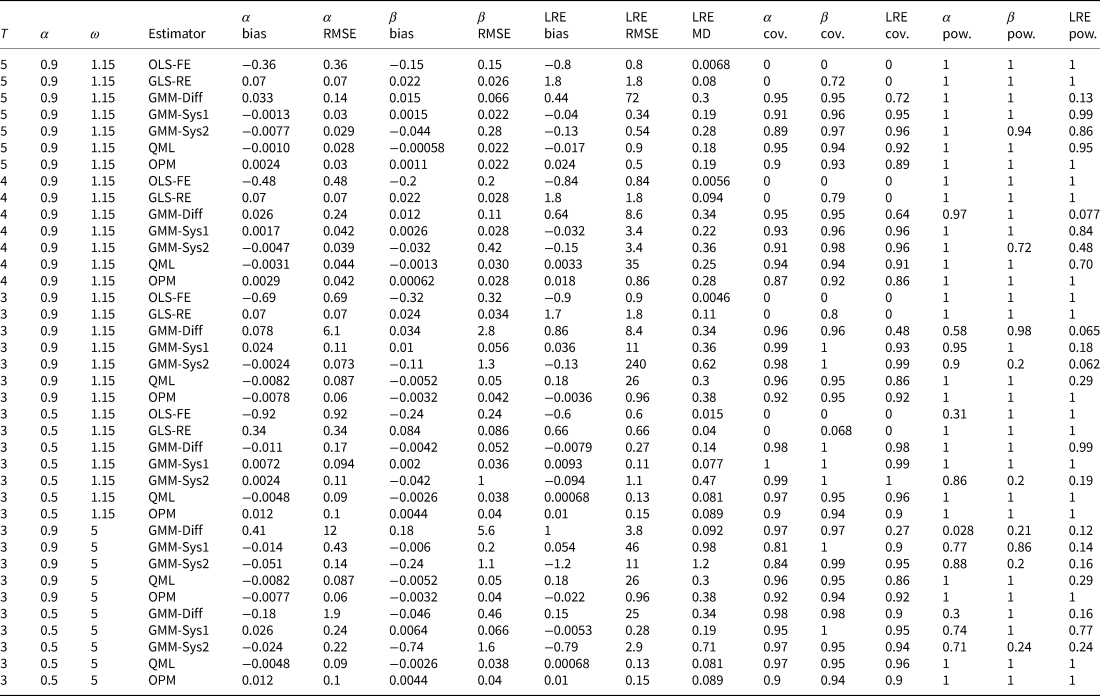
Table 1 presents the results from the Monte Carlo experiment. The mean biases for β and α are both reported. The α coefficient is important because β is only the estimate of the SRE and the full LRE is a function of α: β/(1 − α). The division by (1 − α) means that small errors in α can translate into large errors in the estimated LRE. To demonstrate this, Table 1 also reports the LRE bias. Note that because the estimates of α and β are not independent, the bias in the LRE cannot be determined simply by dividing the β bias by one minus the α bias. Also note that because the LRE is a nonlinear combination of parameters, its distribution is not necessarily symmetric and so we report the median bias in place of mean bias. The root mean squared error for β, α, and the LRE are also reported. The RMSE is an indicator of efficiency and is important because even if an estimator produces the correct answer on average, if it produces a wide range of values, many falling far from the truth, it may be of less value to us than an estimator with a small bias but a narrower range of values. For the LRE, we also report the median deviation from the median estimate (MD). The table reports the biases, RMSEs, and MDs as proportions of the true value. The absolute values are reported in Appendix E. Finally, the proportion of 95 percent confidence intervals that include the true value (the coverage probability statistic) and exclude 0 (the power statistic) are reported. An unbiased estimator that produces accurate standard errors should include the true value within this confidence interval 95 percent of the time and ideally exclude 0, when that is not the true value, 100 percent of the time. These measures reflect the value of the estimator for testing hypotheses regarding the parameter values.

Table 1.

Large N properties (N = 1000)

We begin with a summary of the problems encountered by OLS-FE and GLS-RE. The α bias for each is substantial. For OLS-FE, it ranges from 36 to 69 percent of the true value of the parameter. For GLS-RE, it can be as small as 7 percent but can also be as large as 19 percent of the true value. For β (the SRE), the biases are smaller but still up to 32 percent for OLS-FE. Further, biases in α translate into large LRE bias tables for both estimators. It gets up to 1.8 times the true value for GLS-RE.

Beyond bias, the coverage statistics for α, β, and the LRE are always below the 0.95 target for both OLS-FE and GLS-RE, often close to or equal to zero. These problems remain whether α = 0.5 or 0.9. In contrast, TLEs outperform OLS-FE and GLS-RE in each and every way. It is to these estimators and GMM we now turn.

We start with α = 0.9 and ω = 1.15 and note that the RMSEs for β are greatest for GMM-Diff and GMM-Sys2. The RMSEs increase as T decreases from 28 percent of the true value to 130 percent for GMM-Sys2 and from 6.6 to 280 percent for GMM-Diff. This means this estimator regularly produces SRE estimates that are one to three times too large or small. For the TLEs and the GMM-Sys1 estimator, the biases and RMSEs for β are generally always small, although the OPM RMSEs and biases are always equal to or smaller than the GMM and QML-FE estimators. Larger differences between the estimators are apparent in the estimates of α and therefore the LRE.

As T decreases from 5 to 3 (α = 0.9; ω = 1.15), the α bias(RMSE) for GMM-Diff increases from 3.3 percent(14 percent) to 7.8 percent(6 times the true value). This is due to the weakness of the moment conditions available to GMM-Diff when α is close to 1 (Stock et al., Reference Stock, Wright and Yogo2002) and T is small. Because of the weak instrument problem, GMM-Diff periodically produces a very poor estimate for α. Because of the division by (1 − α) when estimating the LRE, the result is large biases (44 to 86 percent) and extreme RMSEs (many times the true value). Note that unlike the rest of the simulation statistics, the LRE RMSE can be somewhat sensitive to the initial conditions of the simulations. However, it is only sensitive to the extent that when the RMSE is many times the true value, the choice of initial conditions affects how many times greater (but the RMSE is always very large). Under these circumstances it is useful to look at the MD. This is much smaller. However, this does not negate the fact that GMM-Diff periodically produces very poor estimates. This also sometimes results in low power for the LRE (as low as 6.5 percent).

At T = 5, the α and the LRE results for the TLEs and GMM-Sys estimators look much better. The biases are small; the RMSEs are many times smaller than for GMM-Diff; the coverage statistics are around 0.95; and the power is about 1.0 (0.86 for GMM-Sys2). As T is reduced to 4 and then 3, GMM-Sys1 and GMM-Sys2 exhibit only moderate RMSEs for α (up to 11 percent) but this translates into large RMSE (many times the true value) and poor power (as low as 6 percent) for the LRE. QML-FE also has a high RMSE and low-power for LRE. Hsiao et al. (Reference Hsiao, Pesaran and Tahmiscioglu2002) notes that QML-FE does not estimate the LRE well when α is greater than 0.8 and both T and N are small. It would appear that this is also the case when N is large and T is small. Importantly, OPM shows no such biases, has relatively small RMSEs and full power for all parameters. Perhaps because of the way it estimates the LRE, OPM appears much more robust to the problems GMM and QML-FE estimators encounter when T < 5 and α → 1.

When α = 0.5, all GMM and TLE estimators perform well even when T = 3, confirming the problems are a result of α → 1. However, when ω is increased, the RMSEs for all GMM parameter estimates increase (sometimes significantly) regardless of α, while the TLEs are unaffected. This is consistent with the finding that GMM can encounter weak instrument problems when the between variance is large relative to the within variance.

Previous work in Political Science (e.g. Wawro, Reference Wawro2002, 47) suggest 4–5 waves of data are preferable for GMM. With T = 5, and N is large, GMM-Sys1 (and GMM-Sys2 to a lesser extent) resolves many of the problems GMM-Diff exhibits when α is close to 1. GMM-Sys1 is, so far, the optimal GMM estimator, given the DGP. However, all three GMM estimators used valid moment conditions and pass the Sargan test with the expected false rejection rate. Further, even GMM-Sys1 has poor properties for the LRE when T < 5 and α is close to 1. Given one can never know the true value of α in the DGP of real-world data, researchers should consider OPM when they only have 3 or 4 waves of data. This is not an uncommon situation. Of the studies in our literature review 23 percent of them had just three waves. OPM not only performs better under these circumstances, it performs at least as well as other estimators when T > 4 and α is not close to 1.

These conclusions are based on a DGP with a large N but many political science examples of small T panel data do not have a large N. Of the studies in our literature review with T ≤ 10, 38 percent had an N < 500 and in almost half of these, N was less than 50.

5.2 Finite sample properties

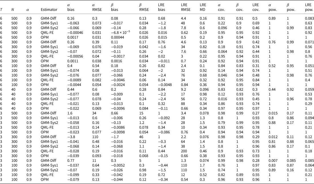
GMM is known to have poor finite sample properties (Bond and Windmeijer, 2002) and Hsiao et al. (Reference Hsiao, Pesaran and Tahmiscioglu2002) find that QML-FE consistently performs better than GMM when both T and N are small. However, they also find that when α > 0.8, QML-FE performs poorly when estimating the LRE. QML-FE sometimes does not even converge under such circumstances. The finite sample properties of OPM are entirely unknown. We repeat our simulations with the same DGP as before but with N = 40, 100, 300, and 500; T = 3 and 6; and α = 0.9. We use ω = 5, making between variance 60 percent greater than within variance—not unusual in political science examples. Appendix E contains the results for ω = 1.15. The results are the same but muted. GMM-Sys1 sometimes ran into problems when optimizing the weighting matrix. When this occurred, the results for that particular data set were dropped from the analysis. In principle, QML-FE could run into convergence problems but it did not during our simulations.

With T = 6 and α = 0.9, GMM-Diff exhibits increasing bias for α and the LRE, as N decreases from 500 to 40. The bias in α increases from 16 to 44 percent. The bias in the LRE increases from 68 to 84 percent. The LRE RMSE increases from 4.4 to 9.2 times the true value. When T = 3, the LRE bias is 100 percent and even at T = 500, the RMSEs for all parameters (including β) are many times the true values. The improved performance of GMM-Sys1 and GMM-Sys2 relative to GMM-Diff in estimating α is similar to that demonstrated by Blundell and Bond (Reference Blundell and Bond1998) but GMM-Sys2 exhibits increasing β RMSEs as T decreases—around 24 percent when T = 6 and 110 percent when T = 3. Also, as demonstrated by Hsiao et al. (Reference Hsiao, Pesaran and Tahmiscioglu2002), the QML-FE RMSEs for α and β are often smaller than they are for the GMM estimators but not consistently for α. The OPM RMSEs are consistently the smallest of all estimators. This efficiency of OPM relative to the GMM estimators as $T \& N \rightarrow 0$ is evident but the starkest differences are in the LRE estimates.

Starting with T = 6, N = 500, the overall best-performing GMM estimator (GMM-Sys1) exhibits a downward LRE bias of 120 percent. As N decreases to 300, then 100 and then 40, the bias increases to 160 percent, then 240 percent. Meanwhile, the RMSEs are many times the true value, and the power drops from 63 to 31 percent. QML-FE exhibits a similar pattern, although with smaller biases. This is consistent with Hsiao et al. (Reference Hsiao, Pesaran and Tahmiscioglu2002). QML-FE also has smaller MDs than the GMMs. OPM biases and RMSEs are consistently many times smaller than even QML-FE, and like QML-FE, the MDs are smaller than the GMMs. Even when N = 40, the LRE bias is only 11 percent, the RMSE 66 percent, and the MD 34 percent. Noticeably, the power never drops below 100 percent.

When T = 3 and N drops to 500, 300, and then 100, the pattern is similar except more extreme. The GMM RMSEs reach 110 times the true value for the LRE, and the power is about 6 percent. For QML-FE, the LRE bias increases from 34 to 72 percent, the LRE RMSE increases from 10 to 12 times the true value, and the LRE power is about 20 percent. For OPM, the LRE bias and RMSE are much smaller. The LRE bias does increase from 9 to 34 percent but even then the RMSE is only 54 percent and the MD 30 percent. Unlike the other estimators, the power for the OPM LRE always remains at 100 percent.

Overall, we see GMM-Diff has poor finite sample properties when α → 1. GMM-Sys1 (and GMM-Sys2 to a lesser extent) is an improvement but has problems estimating the LRE, and as $T \& N \rightarrow 0$, it exhibits increasing RMSEs for all parameters. (And note, we have used a moderate between- to within-variance ratio. As this gets larger, the GMM RMSEs for all parameters are expected to increase further, while the TLEs are unaffected.) QML-FE is somewhat more efficient than GMM when estimating α and β under these conditions but runs into the same trouble estimating the LRE. OPM appears to improve on both the QML-FE and GMM estimators by being more efficient and much more robust in estimating the LRE when α is close to 1 (Table 2).

Table 2.

Finite sample properties

5.3 Violations of distributional assumptions

Up to this point, the DGPs we have used meet the distributional assumptions of TLEs. It is not known how well these estimators perform when these distributional assumptions are violated. Next we use DGPs that violate these assumptions in ways that we might expect to encounter in real-world analyses: outliers in the data; skewed variables; bimodal variables; and heteroskedastic errors.

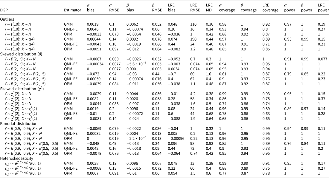
To test the consequences of outliers, we: (1) use the same DGP as in Equation 15 with α = 0.9, and T = 3 but we use a t-distribution with 10 degrees of freedom to generate the error term for Y _it; and (2) we use a t-distribution with 10 degrees of freedom to generate the error term for Y _it, while using a t-distribution with 4 degrees of freedom to generate the error term for X _it. These distributions have the very fat tails that would result from outliers. To test the consequences of skewed data, we: (1) use a beta(2,9) distribution for Y _it; (2) use a beta(2,9) distribution for Y _it and a beta(2,5) distribution for X _it; (3) use a χ²(2) distribution for Y _it; and (4) use a χ²(2) distribution for Y _it and a χ²(2) distribution for X _it. To test the consequences of a bimodal distribution, we: (1) use a beta(0.9,0.9) distribution for Y _it; and (2) use a beta(0.9,0.9) distribution for Y _it and a beta(0.5,0.5) distribution for X _it. To test the consequences of heteroskedastic errors, we generate ε _1,i,t as $e^{( 0.2 \times x_{i, t}) } N( 0,\; \, 1)$.

In each case (Table 3), OPM is largely unbiased and has good power but there are instances (heteroskedastic and χ² distributed errors) when the coverage statistics are as low as 65 percent. QML-FE, on the other hand, sometimes exhibits large LRE bias (60 percent when both Y _it and X _it are χ² distributed) and large RMSEs (although MDs are not large). GMM exhibits such biases less often than QML-FE but the LRE RMSEs are just as large. When OPM exhibits poor coverage statistics, GMM does not but the trade-off is that GMM under these same circumstances has poor power, while OPM does not. For the distributional assumption violations we have identified, it would appear that OPM is largely (but not entirely) robust, while QML-FE and GMM exhibit the same problems of estimating the LRE when T = 3 and α → 1, as they did without the violations.

Table 3.

Violations of distributional assumptions (T = 3; N = 1000)